Forecasting Road Traffic Deaths in Thailand: Applications of Time-Series, Curve Estimation, Multiple Linear Regression, and Path Analysis Models


Abstract
1. Introduction
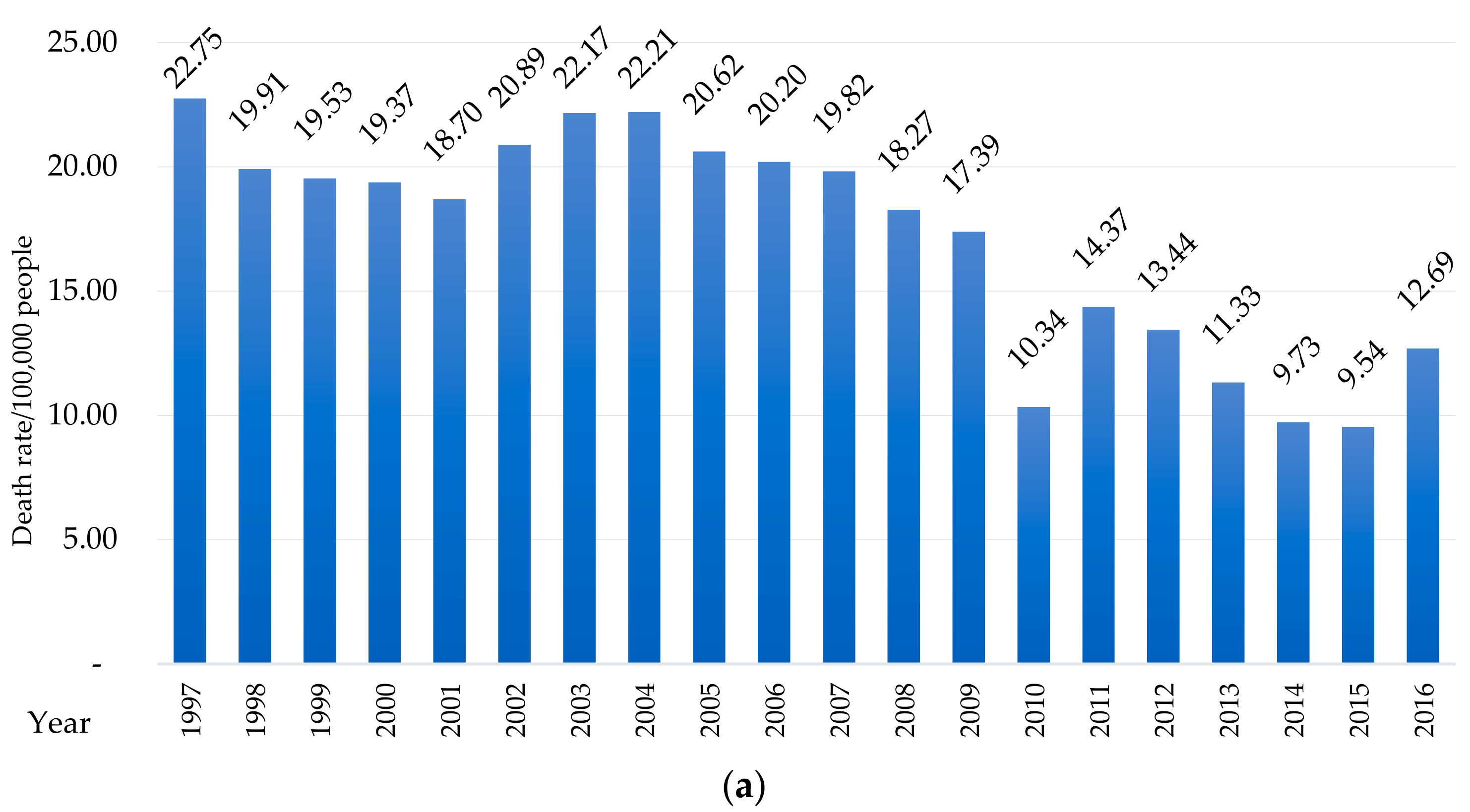
1.1. Road Safety Situation in Thailand
1.2. Importance of Accident Prediction
1.3. Previous Study in Road Accident Prediction
2. Materials and Methods
2.1. Data Collection
2.2. Methodology
2.3. Data Analysis
2.3.1. Time-Series
Model Specification
Model Fitting and Validation
2.3.2. Curve Estimation
2.3.3. Multiple Regression Analysis
2.3.4. Path Analysis
2.3.5. Evaluating Model Efficiency
3. Results
3.1. Statistical Results
3.1.1. Time-Series Data Analysis
3.1.2. Curve Estimation Technique
3.1.3. Multiple Regression Analysis
3.1.4. Path Analysis
3.2. Comparison of Model Performance
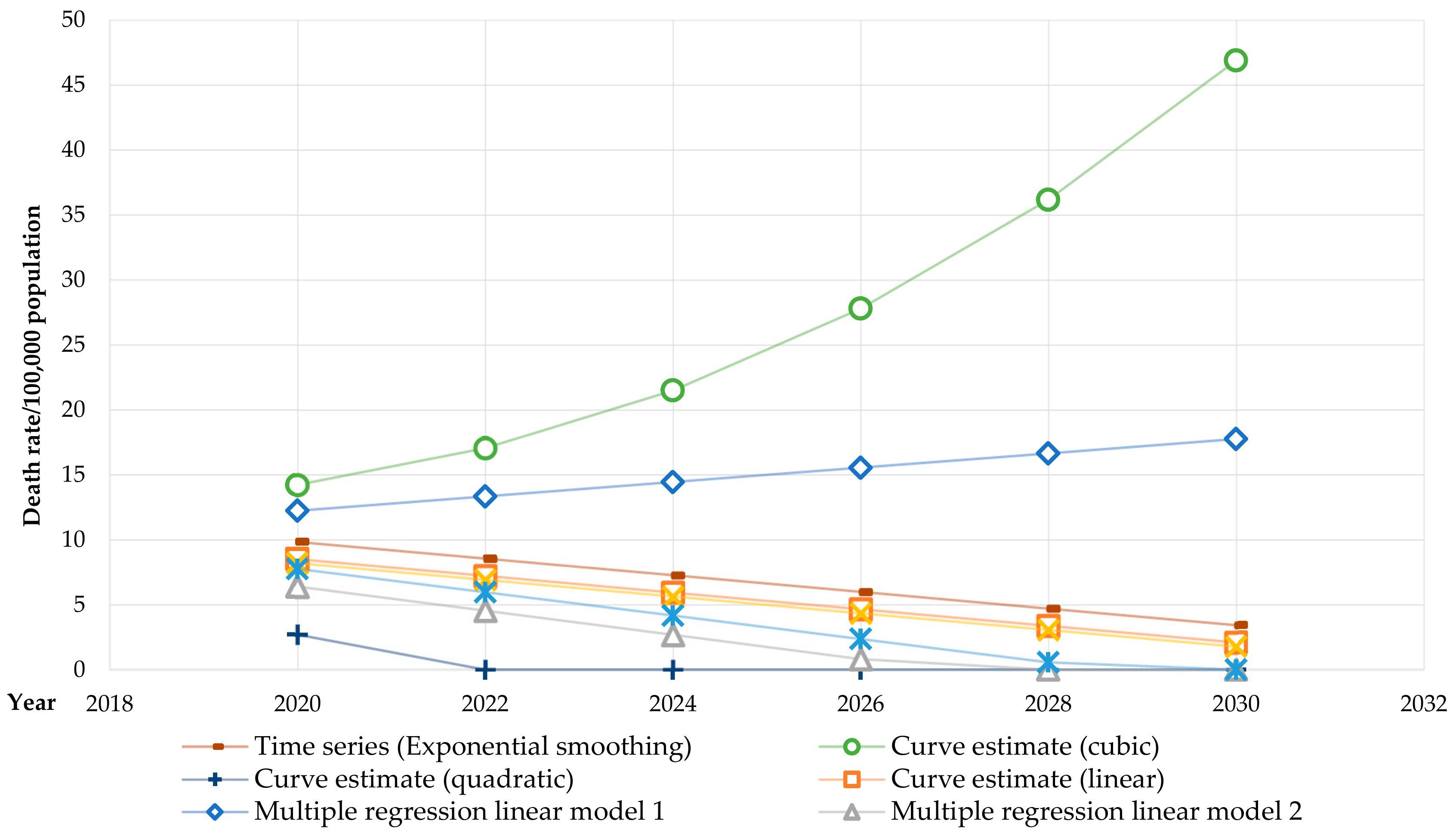
3.3. Forecasting the Death Rate from Road Accidents per 100,000 Population
4. Discussion
- (1)
- The time-series model using exponential smoothing is suitable for predicting the death rate from road accidents. Time-series techniques have also been used to forecast accidents by ARIMA [9,10,11,12,16]. However, the Thai data set was not suitable for the ARIMA technique. The exponential smoothing technique yielded MAE and MAPE values of 1.627 and 8.1%, respectively.
- (2)
- Curve estimation with cubic, quadratic, and linear patterns were the three models with the highest R2 values.
- (3)
- Multiple regression linear model 1 found that GDP was a good economic indicator, in agreement with a previous report by Dadashova et al. [16], and that the transport sector energy consumption level affected the death rate from road accidents, in agreement with reported results García-Ferrer et al. [12]; the number of registered vehicles (motorcycle, cars, and trucks) had no effect.
- (4)
- Using multiple regression linear model 2 (where the proportion of various factors was adjusted by population), we found that the number of registered vehicles and transport sector energy consumption affected the death rate from road accidents, whereas, the other factors had no effect.
- (5)
- Using multiple regression linear model 3 (where the proportion of factors was adjusted for the number of registered vehicles), we found that the number of registered vehicles, number of registered trucks, and the amount of energy consumed by the transport sector affected the death rate from road accidents, whereas, the other factors had no effect.
- (6)
- The path analysis model showed that GDP, energy consumption, and the number of registered vehicles were factors that directly influenced the road death rate. The amount of energy consumed by the transport sector was a factor influenced by the GDP, which indirectly affected the number of road deaths.
5. Limitations and Future Work
Author Contributions
Funding
Acknowledgments
Conflicts of Interest
References
- WHO. Global Status Report on Road Safety 2015; World Health Organization: Geneva, Switzerland, 2015; p. 340. [Google Scholar]
- James Burton, W. Top 25 Countries in Car Accidents. Available online: https://www.worldatlas.com/articles/the-countries-with-the-most-car-accidents.html (accessed on 27 April 2018).
- WHO. World Health Statistics 2017: Monitoring Health for the SDGs, Sustainable Development Goals; World Health Organization: Geneva, Switzerland, 2017. [Google Scholar]
- Department of Disease Control. Road Traffic Death Data Integration: RTDDI, Retroactive Annual Fatality. Available online: http://rti.ddc.moph.go.th/RTDDI/Modules/About.aspx (accessed on 9 February 2018).
- Ministry of Public Health. Public Health Statistics A.D.; Strategy and Planning Division, Ministry of Public Health: Mueang Nonthaburi, Thailand, 2016.
- Royal Thai Police. Traffic Accident on National Highways in 2016. Available online: https://www.m-society.go.th/ewt_news.php?nid=19593 (accessed on 30 October 2018).
- ThaiRSC. Statistics of Traffic Accident Provincial Level. Available online: http://www.thairsc.com/ (accessed on 9 February 2018).
- Brian Bass. Advantages and Disadvantages of Forecasting Methods of Production and Operations Management. Available online: http://smallbusiness.chron.com/advantages-disadvantages-forecasting-methods-production-operations-management-19309.html (accessed on 9 February 2018).
- Quddus, M.A. Time series count data models: An empirical application to traffic accidents. Accid. Anal. Prev. 2008, 40, 1732–1741. [Google Scholar] [CrossRef] [PubMed]
- Ramstedt, M. Alcohol and fatal accidents in the United States—A time series analysis for 1950–2002. Accid. Anal. Prev. 2008, 40, 1273–1281. [Google Scholar] [CrossRef] [PubMed]
- Dadashova, B.; Arenas-Ramírez, B.; Mira-McWilliams, J.; Aparicio-Izquierdo, F. Methodological development for selection of significant predictors explaining fatal road accidents. Accid. Anal. Prev. 2016, 90, 82–94. [Google Scholar] [CrossRef] [PubMed]
- García-Ferrer, A.; de Juan, A.; Poncela, P. Forecasting traffic accidents using disaggregated data. Int. J. Forecast. 2006, 22, 203–222. [Google Scholar] [CrossRef]
- Zheng, X.; Liu, M. An overview of accident forecasting methodologies. J. Loss Prev. Process Ind. 2009, 22, 484–491. [Google Scholar] [CrossRef]
- Sanusi, R.; Adebola, F.B.; Adegoke, N. Cases of Road Traffic accidents: A Time Series Approach. Mediterr. J. Soc. Sci. 2016. [Google Scholar] [CrossRef]
- Parvareh, M.; Karimi, A.; Rezaei, S.; Woldemichael, A.; Nili, S.; Nouri, B.; Nasab, N.E. Assessment and prediction of road accident injuries trend using time-series models in Kurdistan. Burn. Trauma 2018, 6, 9. [Google Scholar] [CrossRef] [PubMed]
- Dadashova, B.; Ramírez Arenas, B.; McWilliams Mira, J.; Izquierdo Aparicio, F. Explanatory and prediction power of two macro models. An application to van-involved accidents in Spain. Transp. Policy 2014, 32, 203–217. [Google Scholar] [CrossRef]
- Michalaki, P.; Quddus, M.A.; Pitfield, D.; Huetson, A. Exploring the factors affecting motorway accident severity in England using the generalised ordered logistic regression model. J. Saf. Res. 2015, 55, 89–97. [Google Scholar] [CrossRef] [PubMed]
- Lu, P.; Tolliver, D. Accident prediction model for public highway-rail grade crossings. Accid. Anal. Prev. 2016, 90, 73–81. [Google Scholar] [CrossRef] [PubMed]
- Oh, J.; Washington, S.P.; Nam, D. Accident prediction model for railway-highway interfaces. Accid. Anal. Prev. 2006, 38, 346–356. [Google Scholar] [CrossRef] [PubMed]
- Ameen, J.R.M.; Naji, J.A. Causal models for road accident fatalities in Yemen. Accid. Anal. Prev. 2001, 33, 547–561. [Google Scholar] [CrossRef]
- Department Provincial Administration. Official Statstics Registration Sytstems. Available online: https://www.dopa.go.th/main/web_index (accessed on 23 August 2017).
- Bank of Thailand. Thailand’s Macro Economic Indicators 1; Bank of Thailand: Bangkok, Thailand, 2016. [Google Scholar]
- Department of Land Transport. Transport Statistics. Available online: http://apps.dlt.go.th/statistics_web/vehicle.html (accessed on 9 February 2018).
- Ministry of Energy. Department of Alternative Energy Development and Efficiency, Energy Statistics & Information, Energy Consumption for Transport Sector. Available online: http://www.dede.go.th/ewt_news.php?nid=42079 (accessed on 9 February 2018).
- Dielman, T.E. Applied Regression Analysis, 4th ed.; Curt Hinrichs: Cincinnati, OH, USA, 2005. [Google Scholar]
- Roberts, S.W. Control Chart Tests Based on Geometric Moving Averages. Technometrics 1959, 1, 239–250. [Google Scholar] [CrossRef]
- Ott, R.L.; Longnecker, M.T. An Introduction to Statistical Methods and Data Analysis, 6th ed.; Brooks/Cole: Pacific Grove, CA, USA, 2010; p. 1296. [Google Scholar]
- Hair, J.F.; Black, W.C.; Babin, B.J.; Anderson, R.E. Multivariate Data Analysis: A Global Perspective; Pearson Education: London, UK, 2010; p. 800. [Google Scholar]
- Ratanavaraha, V.; Jomnonkwao, S. Trends in Thailand CO2 emissions in the transportation sector and Policy Mitigation. Transp. Policy 2015, 41, 136–146. [Google Scholar] [CrossRef]
- Muthén, L.K.; Muthén, B.O. Mplus User’s Guide, 7th ed.; Muthén & Muthén: Los Angeles, CA, USA, 1998–2012; p. 850. [Google Scholar]
- Kline, R.B. Principles and Practice of Structural Equation Modeling; Guilford Press: New York, NY, USA, 2011. [Google Scholar]
- Steiger, J.H. Understanding the limitations of global fit assessment in structural equation modeling. Personal. Individ. Differ. 2007, 42, 893–898. [Google Scholar] [CrossRef]
- Hu, L.T.; Bentler, P.M. Cutoff criteria for fit indexes in covariance structure analysis: Conventional criteria versus new alternatives. Struct. Equ. Modeling Multidiscip. J. 1999, 6, 1–55. [Google Scholar] [CrossRef]
- Hooper, D.; Coughlan, J.; Mullen, M.R. Structural Equation Modelling: Guidelines for Determining Model Fit. Electron. J. Bus. Res. Methods 2008, 6, 53–61. [Google Scholar]
- Jomnonkwao, S.; Sangphong, O.; Khampirat, B.; Siridhara, S.; Ratanavaraha, V. Public transport promotion policy on campus: Evidence from Suranaree University in Thailand. Public Transp. 2016, 8, 185–203. [Google Scholar] [CrossRef]


| Author | Period | Methodology | Data | |||||||||
|---|---|---|---|---|---|---|---|---|---|---|---|---|
| Time-Series | Regression | Other | Accident Data | Environment Conditions | Economic Factors | Energy Consumption | Alcohol Consumption | Law | Vehicle Registration | Population | ||
| Quddus [9] | 1950–2005 (55 years) | ✓ | - | - | ✓ | ✓ | - | - | - | ✓ | - | - |
| Michalaki, et al. [17] | 2005–2011 (6 years) | - | ✓ | - | ✓ | ✓ | - | - | - | - | - | - |
| Lu and Tolliver [18] | 1996–2014 (18 years) | - | ✓ | ✓ | ✓ | ✓ | - | - | - | - | - | - |
| Ramstedt [10] | 1950–2002 (52 years) | ✓ | - | ✓ | ✓ | - | - | - | ✓ | - | - | - |
| Oh, et al. [19] | 1998–2002 (4 years) | - | ✓ | ✓ | ✓ | ✓ | - | - | - | - | - | - |
| Dadashova, et al. [11] | 2000–2011 (11 years) | ✓ | - | - | ✓ | ✓ | ✓ | - | - | ✓ | - | - |
| Dadashova, et al. [16] | 2000–2009 (9 years) | ✓ | - | ✓ | ✓ | ✓ | ✓ | - | - | ✓ | - | - |
| García-Ferrer, et al. [12] | 1975–2003 (28 years) | ✓ | ✓ | - | ✓ | - | ✓ | ✓ | - | - | ✓ | - |
| Zheng and Liu [13] | 1989–2002 (13 years) | ✓ | ✓ | ✓ | ✓ | - | - | - | - | - | - | - |
| Ameen and Naji [20] | 1978–1995 (17 years) | - | ✓ | - | ✓ | ✓ | ✓ | - | - | - | ✓ | ✓ |
| Sanusi, et al. [14] | 1969–2013 (54 years) | ✓ | - | - | ✓ | - | - | - | - | - | - | - |
| Parvareh, et al. [6,15] | 2009–2015 (72 months) | ✓ | - | - | ✓ | - | - | - | - | - | - | - |
| This research | 1997–2016 (20 years) | ✓ | ✓ | Curve estimate, Path analysis | ✓ | - | ✓ | ✓ | - | - | ✓ | ✓ |
| Model | R2 | Adjusted R2 | SE of the Estimate | F | Equation |
|---|---|---|---|---|---|
| Linear | 0.738 | 0.724 | 2.318 | 50.815 | E(y)t = 23.879 − 0.641T |
| Logarithmic | 0.511 | 0.483 | 3.170 | 18.785 | E(y)t = 25.361 − 3.878ln(T) |
| Inverse | 0.249 | 0.208 | 3.926 | 5.981 | E(y)t = 15.379 + (9.856/T) |
| Quadratic | 0.816 | 0.794 | 2.001 | 37.638 | E(y)t = 20.772 + 0.207T − 0.040T2 |
| Cubic | 0.842 | 0.813 | 1.908 | 28.511 | E(y)t = 18.262 + 1.487T − 0.189T2 + 0.005T3 |
| Compound | 0.729 | 0.714 | 0.152 | 48.518 | E(y)t = 25.494(0.960)T |
| Power | 0.489 | 0.460 | 0.210 | 17.210 | E(y)t = 27.813T−0.245 |
| S | 0.223 | 0.180 | 0.258 | 5.179 | E(y)t = exp[2.698 + (0.603/T)] |
| Growth | 0.729 | 0.714 | 0.152 | 48.518 | E(y)t = exp[3.238 − (0.041T)] |
| Exponential | 0.729 | 0.714 | 0.152 | 48.518 | E(y)t = 25.494exp−0.041T |
| Variable | Model 1 | ||
| (Y = Death Rate/100,000 Population) | |||
| B | t-Statistic | p-Value | |
| VEH_MOTORCYCLE | - | - | - |
| VEH_CAR | - | - | - |
| VEH_TRUCK | - | - | - |
| GDP | −2.393 × 10⁻⁶ | −5.551 | <0.001 ** |
| EN_TRANSPORT | 0.001 | 2.839 | <0.05 * |
| Constant | 12.838 | 2.370 | <0.05 * |
| F-test | 51.814 | ||
| Adjusted R2 | 0.842 | ||
| Variables | Model 2 | ||
| (Y = Death Rate/100,000 Population) | |||
| B | t-Statistic | p-Value | |
| VEH_MOTORCYCLE/1,000 population | - | - | - |
| VEH_CAR/1,000 population | −0.127 | −6.405 | <0.001 ** |
| VEH_TRUCK/1,000 population | - | - | - |
| GDP/1,000 population | - | - | - |
| EN_TRANSPORT/100,000 population | 0.424 | 2.265 | <0.001 ** |
| Constant | 19.632 | 4.399 | <0.001 ** |
| F-test | 55.915 | ||
| Adjusted R2 | 0.853 | ||
| Variables | Model 3 | ||
| (Death Rate/100,000 Population) | |||
| B | t-Statistic | p-Value | |
| VEH_MOTORCYCLE/1,000 VEH_TOTAL | - | - | - |
| VEH_CAR/1,000 VEH_TOTAL | −0.081 | −8.769 | <0.001 ** |
| VEH_TRUCK/1,000 VEH_TOTAL | −0.723 | −2.266 | <0.05 * |
| GDP/1,000 VEH_TOTAL | - | - | - |
| EN_TRANSPORT/1,000 VEH_TOTAL | 0.260 | 4.006 | <0.001 ** |
| Constant | 42.096 | 5.903 | <0.001 ** |
| F-test | 51.144 | ||
| Adjusted R2 | 0.888 | ||
| Relationship | Model Stat | |||
|---|---|---|---|---|
| B (β) | SE | t-Statistic | p-Value | |
| GDP → FA_RATE | −0.106 (−0.193) | 0.033 (0.352) | −3.245 (−3.390) | <0.05 *(<0.05 *) |
| EN_TRANSPORT → FA_RATE | 0.834 (0.992) | 0.214 (0.274) | 3.896 (3.615) | <0.001 **(<0.001 **) |
| VEH_MOTORCYCLE → FA_RATE | 0.041 (0.432) | 0.022 (0.233) | 1.881 (1.857) | 0.060 (0.063) |
| VEH_CAR → FA_RATE | −0.120 (−1.485) | 0.060 (0.747) | −2.021 (−1.989) | <0.05 *(<0.05 *) |
| VEH_TRUCK → FA_RATE | 0.690 (0.396) | 1.073 (0.614) | 0.643 (0.645) | 0.520 (0.519) |
| EN_TRANSPORT → GDP | 8.898 (0.938) | 0.734 (0.027) | 12.120 (35.012) | <0.001 **(<0.001 **) |
| VEH_MOTORCYCLE→ EN_TRANSPORT | −0.044 (−0.388) | 0.027 (0.240) | −1.623 (−1.615) | 0.105 (0.106) |
| VEH_CAR → EN_TRANSPORT | 0.137 (1.420) | 0.074 (0.752) | 1.863 (1.888) | 0.062 (0.059) |
| VEH_TRUCK → EN_TRANSPORT | −0.345 (−0.166) | 1.411 (0.680) | −0.0244 (−0.244) | 0.807 (0.807) |
| Intercept | ||||
| FA_RATE | −0.799 (−0.194) | 10.513 (2.554) | −0.076 (−0.076) | 0.939 (0.939) |
| GDP | −187.266 (−4.035) | 27.035 (0.639) | −6.927 (−6.317) | <0.001 **(0.001 **) |
| EN_TRANSPORT | −0.345 (6.629) | 10.361 (0.680) | 3.131 (2.783) | <0.05 *(<0.05 *) |
| Residual variances | ||||
| FA_RATE | −2.262 (0.134) | 0.715 (0.055) | 3.162 (2.430) | <0.05 *(<0.05 *) |
| GDP | 258.150 (0.120) | 81.634 (0.050) | 3.162 (2.383) | <0.05 *(<0.05 *) |
| EN_TRANSPORT | 4.040 (0.169) | 10.361 (0.069) | 3.162 (2.452) | <0.05 *(<0.05 *) |
| R2 | ||||
| FA_RATE | 0.866 | 0.055 | 15.739 | <0.001 ** |
| GDP | 0.880 | 0.050 | 17.506 | <0.001 ** |
| EN_TRANSPORT | 0.831 | 0.069 | 12.087 | <0.001 ** |
| Model | Year | Value | ||||||
|---|---|---|---|---|---|---|---|---|
| 1997 | 2001 | 2006 | 2011 | 2016 | MAE * | MAPE * | ||
| 1 | Time-series (exponential smoothing) | 22.53 | 18.68 | 20.05 | 11.78 | 9.09 | 1.62 | 8.1 |
| 2 | Curve estimate (cubic) | 19.57 | 21.60 | 19.23 | 14.92 | 12.40 | 2.23 | 11.2 |
| 3 | Curve estimate (quadratic) | 20.94 | 20.81 | 18.84 | 14.88 | 8.91 | 2.04 | 10.2 |
| 4 | Curve estimate (linear) | 23.24 | 20.67 | 17.47 | 14.26 | 11.06 | 2.52 | 12.6 |
| 5 | Multiple regression linear model 1 | 21.82 | 18.68 | 15.72 | 11.26 | 11.87 | 2.56 | 12.8 |
| 6 | Multiple regression linear model 2 | 23.20 | 19.08 | 18.44 | 14.19 | 7.67 | 1.91 | 9.5 |
| 7 | Multiple regression linear model 3 | 23.65 | 19.26 | 19.13 | 14.97 | 10.08 | 1.28 | 6.4 |
| 8 | Path analysis | 24.40 | 21.13 | 19.17 | 15.16 | 11.13 | 1.68 | 8.4 |
| Parameter | Year | |||||
|---|---|---|---|---|---|---|
| 2020 | 2022 | 2024 | 2026 | 2028 | 2030 | |
| Population (106) | 66.84 | 67.30 | 67.77 | 68.24 | 68.71 | 69.17 |
| GDP (1012 baht/1000 population); 1997 constant price | 253.17 | 269.79 | 286.41 | 303.04 | 319.66 | 336.28 |
| Motorcycle registration /1000 population | 333.62 | 344.74 | 355.85 | 366.97 | 378.08 | 389.20 |
| Car registration /1000 population | 267.55 | 287.37 | 307.19 | 327.01 | 346.84 | 366.66 |
| Truck registration /1000 population | 17.72 | 18.57 | 19.42 | 20.27 | 21.12 | 21.97 |
| Energy consumption of the transportation sector (Ktoe/100,000 population) | 48.91 | 50.47 | 52.03 | 53.59 | 55.15 | 56.72 |
| Motorcycle/1000 Total Vehicles registered | 516.00 | 502.12 | 488.25 | 474.37 | 460.49 | 446.61 |
| Car/1000 Total Vehicles registered | 428.52 | 441.85 | 455.19 | 468.52 | 481.85 | 495.19 |
| Truck/ 1000 Total Vehicles registered | 26.45 | 25.97 | 25.50 | 25.02 | 24.54 | 24.07 |
| GDP /1000 Total Vehicles registered; 1997 constant price | 425.16 | 443.38 | 461.59 | 479.81 | 498.03 | 516.24 |
| Energy consumption of the transportation sector (Ktoe)/1000 Total Vehicles registered | 76.64 | 74.53 | 72.42 | 70.32 | 68.21 | 66.10 |
| Model | Year | ||||||
|---|---|---|---|---|---|---|---|
| 2020 | 2022 | 2024 | 2026 | 2028 | 2030 | ||
| 1 | Time-series (exponential smoothing) | 9.82 | 8.54 | 7.26 | 5.98 | 4.70 | 3.42 |
| 2 | Curve estimate (cubic) | 14.20 | 17.00 | 21.50 | 27.80 | 36.20 | 46.90 |
| 3 | Curve estimate (quadratic) | 2.70 | - | - | - | - | - |
| 4 | Curve estimate (linear) | 8.50 | 7.21 | 5.93 | 4.65 | 3.37 | 2.09 |
| 5 | Multiple regression linear model 1 | 12.20 | 13.30 | 14.40 | 15.50 | 16.60 | 17.7 |
| 6 | Multiple regression linear model 2 | 6.39 | 4.54 | 2.68 | 0.82 | - | - |
| 7 | Multiple regression linear model 3 | 8.19 | 6.91 | 5.62 | 4.34 | 3.06 | 1.77 |
| 8 | Path analysis | 7.75 | 5.96 | 4.16 | 2.36 | 0.56 | - |
© 2020 by the authors. Licensee MDPI, Basel, Switzerland. This article is an open access article distributed under the terms and conditions of the Creative Commons Attribution (CC BY) license (http://creativecommons.org/licenses/by/4.0/).
Share and Cite
Jomnonkwao, S.; Uttra, S.; Ratanavaraha, V. Forecasting Road Traffic Deaths in Thailand: Applications of Time-Series, Curve Estimation, Multiple Linear Regression, and Path Analysis Models. Sustainability 2020, 12, 395. https://doi.org/10.3390/su12010395
Jomnonkwao S, Uttra S, Ratanavaraha V. Forecasting Road Traffic Deaths in Thailand: Applications of Time-Series, Curve Estimation, Multiple Linear Regression, and Path Analysis Models. Sustainability. 2020; 12(1):395. https://doi.org/10.3390/su12010395
Chicago/Turabian StyleJomnonkwao, Sajjakaj, Savalee Uttra, and Vatanavongs Ratanavaraha. 2020. "Forecasting Road Traffic Deaths in Thailand: Applications of Time-Series, Curve Estimation, Multiple Linear Regression, and Path Analysis Models" Sustainability 12, no. 1: 395. https://doi.org/10.3390/su12010395
APA StyleJomnonkwao, S., Uttra, S., & Ratanavaraha, V. (2020). Forecasting Road Traffic Deaths in Thailand: Applications of Time-Series, Curve Estimation, Multiple Linear Regression, and Path Analysis Models. Sustainability, 12(1), 395. https://doi.org/10.3390/su12010395