Article

Pay Me Later is Not Always Positively Associated with Bank Risk Reduction—From the Perspective of Long-Term Compensation and Black Box Effect

1
School of Management, Harbin Institute of Technology, Harbin City 150000, China
2
School of Business, Singapore University of Social Sciences, Singapore 599494, Singapore
*
Author to whom correspondence should be addressed.
Sustainability 2020, 12(1), 35; https://doi.org/10.3390/su12010035
Submission received: 19 November 2019 / Revised: 11 December 2019 / Accepted: 16 December 2019 / Published: 18 December 2019
(This article belongs to the Special Issue Sustainable Banking: Issues and Challenges)

Abstract

:
The relationship between executive compensation and bank risk-taking is one of the core topics of corporate governance theory. Especially after the 2008 global financial crisis, due to the characteristics of banks, such as systemic risk, this relationship has become more important. However, though usually calculated on the basis of cash salary and inside equity, which can promote risk incentives, inside debt was considered a tool for risk reduction in prior empirical analyses. Based on actual bank situations, we had doubts about this relationship and wanted to verify the specific relationship between inside debt and risk. We initiated this research by setting up a theoretical model between inside debt and bank default risk and by simulating the result using data from Wells Fargo & Co. to draw the function image. We are the first to define the three kinds of compensation in three dimensions. Then, considering bankruptcy, we found the black box effect exists. Therefore, different from prior views, pay me later not only reduces but also increases risk. We expect our findings to offer help to the formulation of policies for pay contracts.

1. Introduction

During the four decades since Jensen and Meckling published their article in 1976 [1], the academic literature on executive compensation has increased. Most of the papers focused predominantly on equity-based compensation (also called “inside equity” here) paid in the form of restricted stock, stock options, and other instruments, of which the value lies in the equity returns in the future. However, Sundaram and Yermack [2] first proposed that chief executive officers (CEOs) with high debt-based compensation (also called “inside debt” here) manage their firms conservatively. Per Jensen and Meckling [1], inside debt is defined as benefit pensions and deferred compensation. Sundaram and Yermack [2] defined inside debt as “the promise to pay them fixed sums of cash in the future”. In this study, we investigated the true relationship of inside debt and bank risk and found the principle and reason for the relationship, proceeding from reality. Figure 1 summarizes the related studies and outlines the framework of our study. We define the total compensation as the sum of cash salary, inside equity, and inside debt from the following aspects: remuneration level, compensation structure level, bank level, measure level, board level, and reform level.
Overall, our study is important for understanding financial stability. Specifically, Abad-Segura et al. [3] raised the obligation of companies to corporate social responsibility from a sustainability approach. Of the unique characteristics of the banking industry, corporate governance in banks is different from that in nonfinancial firms [4]. Banks have various special attributes: their high leverage, their opaqueness, and their systemic risk. In other words, the risk taking of a single bank may result in depression and even collapse of the whole economy, with potential for international consequences (Figure 1, middle right).
The factors influencing bank risk from the perspective of corporate governance include board attributes, remuneration and pay contract, risk management, and the measure of risk.
Firstly, in terms of board attributes, Beltratti and Stulz [5] found that shareholder-friendly boards are positively associated with default risk. Erkens et al. [6] stated that banks with a higher fraction of independent directors reduced leverage risk by raising equity during the 2008 financial crisis. Berger et al. [7] concluded that portfolio risk is positively related to younger executives and female directors. Minton et al. [8] demonstrated the positive association between higher amounts of financial experts and bank risk, including equity risk, leverage risk, and portfolio risk. The International Monetary Fund (IMF) [9] reported that a higher fraction of independent directors is positively associated with lower bank risk. However, the effect of the following remains unknown: nonexecutive directors, the board process, and the joint impact of board attributes and CEO power (Figure 1, upper right).
Secondly, for the remuneration level, Hagendorff and Vallascas [10] reported that high Vega banks pursue acquisitions that result in increasing default risk. DeYoung et al. [11] pointed out that a higher Vega results in shifting the business model of banks to nontraditional activities associated with an increase in equity risk. Galletta and Mazzù [12] created a liquidity mismatch index based on the loan-to-deposit ratio for three different bank business models. The IMF [9] showed that higher equity-based pay is associated with lower bank risk, including default risk, equity risk, and tail risk. Bennett et al. [13] found that higher inside debt was associated with lower default risk during the 2008 financial crisis. van Bekkum [14] and Bolton et al. [15] demonstrated the negative relationship between inside debt and tail risk. Cheng et al. [16] identified that residual compensation is positively related to equity risk (Figure 1, middle left).
Thirdly, on the risk management level, Keys et al. [17] reported that stronger risk management is associated with less risky subprime loan securitizations. Fahlenbrach et al. [18] stated that banks with persistent risk-taking culture performed poorly and were more likely to fail during the 2007–2008 financial crisis. Ellul and Yerramilli [19] reported that a stronger risk management index (RMI) is associated with lower tail risk exposure and better loan quality. RMI was also a strong predictor of bank tail risk exposures during the financial crisis. Köhler et al. [20] studied the impact of business models on bank stability in European Union (EU) countries. The IMF [9] stated that banks with a risk committee are associated with lower risk-taking. The joint impact is still unknown (Figure 1, lower right).
Fourthly, risk can be measured using different methods, for instance, portfolio risk [17], default risk [18], tail risk [19], equity risk [9], and leverage [8] (Figure 1, upper right).
Though usually calculated on the basis of cash salary and inside equity, which can promote risk incentives, inside debt has been almost considered a tool for risk reduction in prior work on empirical analysis. The results reported by Wu [21] further indicate that this positive effect of CEO inside debt is mainly driven by deferred compensation. Srivastav et al. [22] concluded that inside debt can help to address risk-shifting concerns by aligning the interests of CEOs with those of creditors, regulators, and, in the case of TARP banks, the taxpayer. Then, Srivastav et al (2018) [23] sated that banks, when acquiring CEOs, have high inside debt incentives and display lower market measures of risk and lower loss exposures for taxpayers. Reid [24] outlined the best structures of inside debt so that it functions as a resource to manage firm risk. Mo et al. [25] empirically found a positive association between CEO inside debt holdings and long-term horizons. Milidonis et al. [26] identified a significant and negative relationship between CEO inside debt holdings and risk-taking behavior. Deng et al. [27] showed that CEO compensation deferring significantly reduces bank risk-taking in an emerging market. Chen and Fan [28] investigated the effects of a borrowing firm’s CEO inside debt holdings on the structure of the firm’s syndicated loans. Bhandari et al. [29] linked debt-like compensation to financial analyst behavior.
Other aspects of inside debt and its mechanisms influence a bank’s situation. For instance, the results reported by Sheikh [30] suggest that market competition significantly influences the effect of CEO inside debt on corporate risk-taking. Li et al. [31] provided an inside debt metric that is conceptually superior to previously used metrics. Li and Zhang [32] stated that firms with a higher ratio of female directors tend to have a larger proportion of short-maturity debt. Li et al. [33] found that, when a CEO holds a large amount of inside debt, the firm is less likely to issue convertibles than straight debt. Im et al. [34] investigated the impact of CEO inside debt on cost decisions. Freund et al. [35] identified positive relationships between CEO inside debt holdings and the firm’s likelihood to issue debt. Dasgupta et al. [36] reported that employee deposits mitigate firms’ risk-taking behavior and reduce the agency cost of debt. Colonnello et al. [37] showed that the size and seniority of inside debt are crucial in the relationship between inside debt and credit spreads. Chi et al. [38] highlighted the importance of investigating the implication of CEO debt-like compensation for corporate tax policies. Brisker and Wang [39] thought that debt-type compensation (inside debt) exacerbates the divergence in risk preferences, affecting capital structure decisions. Belkhir et al. [40] were the first to examine the relationship between debt-like compensation and excess cash valuation. Beavers [41] found that larger firms with high CEO inside debt have lower interest rates on these debt instruments and shorter maturities. Overall, the above suggest a more conservative financing policy with regards to debt.
However, in practice, only cash salary is paid per year, not inside debt or inside equity. As a consequence, identifying the principle and mechanism of inside debt using empirical analysis with annual data is hard. In the literature, most of the empirical analysis of various remunerations was conducted on an annual basis but only the actual calculation of fixed remuneration was conducted on an annual basis. In reality, inside equity is issued on a recurring basis only when the company’s equity increases and the inside debt is deferred, the value of which is linearly related to the first two. In this study, we aimed to define and distinguish the three types of compensation calculations and the relationship with risk in three dimensions to further analyze the changes in their nature considering bankruptcy and to establish a case with an executive’s tenure as a term. We used CEO compensation and U.S. bank accounting data from the ExecuComp and BvD Orbis databases.
We initiated this research by modeling the theoretical relationship between inside debt and bank default risk. First, if the bank’s possibility of bankruptcy is not considered, the cash salary of bankers is paid per year and is not irrelevant to the bank risk; inside equity is paid per time (usually not by year) and can be considered as a series of sequential call options. Inside debt is paid in the latter part of the banker’s tenure and the calculation of inside debt is linearly related to the sum of cash salary and inside equity per year. Therefore, we defined the three kinds of compensation using three dimensions, inside debt per time, per year, and during the tenure, and complete the same for inside equity and cash salary for the convenience of calculation. After setting the model of inside debt and default risk, we performed a simulation using data from Wells Fargo & Co. to identify further features. Then, considering the possibility of bankruptcy, we attempted to identify further features.
The remainder of this paper is organized as follows. We create a model of long-term debt-based compensation in Section 2. We characterize the function of inside debt and bank default risk and then we analyze the nature of functions and related indicators such as the inside debt Vega V e g a I D and the sensitivity of inside debt S E N I D in Section 3. Since the function is an implicit function of risk, it is impossible to directly write the expression based on the nature of the similarity to the Black Sholes option function (see Black and Sholes (1973) [42]), we drew the fitting graph using Wells Fargo & Co. data in Section 4. We directly obtained some more intuitive features from the figures that are not to obtain from other mathematical methods. The last section concludes the paper.

2. Materials and Methods

Firstly, Table 1 summarizes the notations and definitions in our model.

2.1. Model Assumptions

To develop the banker’s compensation model, we assumed the following:

2.1.1. Meet All Assumptions 1–7 of the BS Model

One of our core ideas is to regard executive compensation as a series of call options, so the relevant assumptions for satisfying the BS option pricing theory (a total of seven) are some of the necessary conditions for the establishment of this model. Assumptions 1–7 are the corresponding assumptions (a)–(g) of Black and Scholes (1973) [42].

2.1.2. Assumption 8

Assumption 8 is the total compensation during the executives’ tenure that consists of three parts: cash salary, inside equity, and inside debt:
T C = C S + I E + I D
where T C is the long-term total compensation of bankers and where C S , I E , and I D are the value of cash salary, inside equity, and inside debt, respectively.
In this paper, inside debt and debt-based compensation are used synonymously, as are inside equity and equity-based compensation.

2.1.3. Assumptions 9–13

Assumption 9: Executives of banks die at exactly the age of 120 years.
Assumption 10: The inside equity frequency is the same as that of inside debt.
Assumption 11: The interval at which each executive receives their inside equity is the same.
Assumption 12: Liquidation is costless and absolute priority holds.
Assumption 13: The banker’s compensation is so small relative to the net assets that its effect on the net asset dynamics can be ignored.
Assumption 9 is the basis upon which the content in Section 2.2.1 is established. Assumptions 10 and 11 create the premise upon which the content in Section 2.2.3 is established. Assumptions 12 and 13 are the necessary conditions for the establishment of Section 2.3.1 and Section 2.3.2, respectively.

2.1.4. Assumption 14

Assumption 14 is the bank operating normally and that no bankruptcy occurs during the banker’s tenure.
The long-term model has two possibilities: bankruptcy and non-bankruptcy. For clarity, the discussion before Section 3.4 argues that the bank will not bankrupt during the executive period, and Section 3.5 and Section 4.3 mainly discuss the possibility of bankruptcy. In other words, at the beginning, we only discuss the relevant nature of inside debt and other kinds of compensation when the risk level is not high enough to cause the bank to go bankrupt. That is to say, Assumption 14 is established, in line with Lemma 1′ and further extended to the broader situation of considering the possibility of bankruptcy. If Assumption 14 is not established, both Lemmas 1 and 1′ are within the scope of discussion.
Lemma 1.
A bank may go bankrupt when
σ θ > P B + G B × ρ
where σ θ is the volatility of R O E , P B is total profits not related to bad debts, G is good credit equity, B is poor credit equity, and ρ is the correlation coefficient between risk and bad debt.
Proof. 
Firstly, bank equity is divided into two parts:
E = G + B × p ( b )
where E is the bank equity; G is good credit equity and B is poor credit equity, which may become part of bad debts (negative); B < 0 ; P B is defined as total profits not related to bad debts; and A s is defined as the bank assets value. Per Roy [43] and Laeven and Levine [44], insolvency is defined as a state in which losses surmount equity:
E < P B
R O E is return on equity and R O E = P B E ; σ θ represents the volatility of R O E . Generally, the larger the volatility of O E ( σ θ ) , the higher the probability of bad debts p ( b ) . Therefore, we assume that a positive relationship exists between the probability of bad debts p ( b ) and
p ( b ) = ρ × σ θ
where ρ is the correlation coefficient between risk and bad debt and where ρ > 0 .
The following formula can be derived from Equations (3) and (5) and from the inequality in Equation (4):
G + B × ρ × σ θ < P B
which can be derived from the inequation in Lemma 1′. □
Similarly, the prerequisite for banks to maintain normal operations is as follows:
Lemma 1′.
When the bank operates normally and no bankruptcy occurs during the executives’ tenure, the bank default risk σ θ satisfies the following:
σ θ P B + G B × ρ
where σ θ is the volatility of R O E , P B is total profits not related to bad debts, G is good credit equity, B is poor credit equity, and ρ is the correlation coefficient between risk and bad debt.
Proof. 
According to Lemma 1, the concept of normal bank operations and bankruptcy, Lemma 1′ is proved as well. □
Although this is not an accurate formula for further calculation, Lemma 1 and Lemma 1′ describe the relationship of σ θ and bankruptcy, lay the foundation for further analysis of the long-term relationship between inside debt and bank default risk, and describe the relationship between inside debt and risk in the case of the possibility of bankruptcy.

2.2. Inside Debt

2.2.1. CEO Pension During Overall Tenure

The debt-based compensation paid to CEOs can take the form of pension benefits, deferred compensations, and even vesting schedules of equity awards for long terms. Since disclosure of the former two items is extremely limited except for pensions, we limited our research to the category of pensions. Therefore, we used the value of pensions to explain the function of inside debt. The following formula was first proposed by Sundaram and Yermack [2]. In most cases, the actuarial present value of the executive’s pension I D is measured as
I D = n = m a x ( 0 , R A ) K A p ( n ) ( I D y ) ( 1 + d ) n
where I D y is the pension amount owed by banks to the bankers per year; R is the minimum age when the banker can choose to retire; A is the current age of the executive, which is a benchmark for using the survival function [45] to estimate p ( n ) ; p ( n ) illustrates the probability of how many years the CEO will live in the future; d is the bank’s long-term debt cost; and K is the last year of the pension, i.e., the final year in their tenure. Since the Social Security Mortality statistical table only shows the mortality rate of people under the age of 120, we assume that executives will all be dead at the age of 120 (Assumption 9). As a consequence, K = 120 and p ( 120 A ) = 0 .

2.2.2. Annual Pension

In practice, per Sundaram and Yermack [2], the annual pension value is often measured using the following formula:
I D y = k = 1 P C t k P × M × S
where C t k is the sum of cash salary and inside equity for year t
C t k = C S y + I E y ,
and P is the past 3 or 5 years during which time cash salary and inside equity are averaged together as part of the equation. M is a multiplier index that is most likely to range from 0.015 to 0.020, and S is the number of working years as a banker. To simplify our calculation, we used the value of cash salary and inside equity to estimate the average of 3 or 5 years, as shown in Equation (11):
I D y = C t k × M × S .
Note that pension is a long-term and a deferred indicator. I D y here is different from not paid per year in practice; I D y represents the base value used to calculate how many pensions should be issued in the future. The value is determined from practice because banks decide how many pensions will be issued in the future on the basis of the annual cash salary ( C S y ) and annual inside equity ( I E y ) . I D y is the annual average, which is assumed to be the same for each year during a banker’s tenure.
To maintain consistency amongst the variables, we used the variables in Equations (8) and (11) to represent the term of the executive. We define the length of the executive’s term as κ from Equations (8) and (11), where S is the working life of the executive, A is the current age, and K is the age of retirement. Then, κ = [ A S , K ] = K A + S . Thus, we have the following:
I D y = I D κ
I D t = I D λ
where I D y is the annual inside debt that is not paid per year but used only for the convenience of calculation and where I D t is the average value of inside debt paid per time. Assume a total of λ times were issued during the term of the executive. This distinction is based on reality and clarifies the model of long-term compensation.

2.2.3. Annual Cash Salary and Annual Inside Equity

Similar to I D y and I D t , we define C S y and C S t as cash salary per year and per time, respectively; I E y and I E t describe inside equity of the average value of each year and each time, respectively. In most conditions, however, different from inside debt and inside equity, cash salary is usually issued once per year. As a consequence, we have the following:
C S y = C S t = C S κ
where C S y is the cash salary per year, which equals the value of cash salary per time C S t . We also have the following:
I E y = I E κ
I E t = Δ ( I E ) κ = I E λ
where λ is the inside equity frequency and this frequency is the same as that of inside debt (Assumption 10). For calculating the banker’s inside equity, tenure [ A S ,   K ] is divided into λ equal length intervals, where λ is bounded and a positive integer, i.e., assuming that the interval at which each executive receives their inside equity is the same (Assumption 11). Moreover, Δ = κ / λ , where Δ is the length of the intervals.

2.2.4. Pension Formula and Structure Coefficient of Pay Contract

The following formula can be derived from Equations (8), (9), (12), (14), and (15):
I D = μ × ( C S + I E )
where μ is the structure coefficient of the pay contract and represents the proportion of inside debt to total compensation using Equation (1)
μ = M S κ n = m a x ( 0 , R A ) K A p ( n ) ( 1 + d ) n
and σ θ P B + G B × ρ (Assumption 14, which will not be repeated as it is emphasized in Section 3.5).
As C S is a fixed value irrelevant to σ θ , I D is converted to the value of I E . We can conclude that
I D y = μ × ( I E y + C S y )
which demonstrates that μ is not only the structure factor of long-term compensation during the banker’s tenure but also that for each time but is not appropriate for each year.
Although the calculation of the value of μ is too cumbersome according to the above formula, it is unrelated to the size of each salary. Therefore, in this study, μ is considered a constant that is unrelated to risk.

2.3. Inside Equity

2.3.1. Inside Equity and Call Option

We used the simple framework introduced by Merton [46] to develop our model. Consider a bank with zero-coupon debt with face value E q ( ( i 1 ) Δ ) , maturity E q ( i Δ ) , and equity for all i { 1 ,   2 , λ } . If the value E q ( i Δ ) of the bank’ s net assets on date κ exceeds E q ( ( i 1 ) Δ ) , the debt is paid off and the balance is paid to the bank’s equity holders. If E q ( i Δ ) < E q ( ( i 1 ) Δ ) , the bank is liquidated. Assume that liquidation is costless and that absolute priority holds (Assumption 12); then, the payoff to equity holders on date κ is as follows:
m a x [ E q ( i Δ ) E q ( ( i 1 ) Δ ) , 0 ]
Suppose the executive holds a fraction ω of the bank’s equity. Time κ payoff to the banker is as follows:
ω m a x [ E q ( i Δ ) E q ( ( i 1 ) Δ ) , 0 ]
The value of the banker’s inside equity can now be determined using the standard option pricing theory of Black and Scholes [42]. If C ( Δ ,   K C ) is the current value of a call option on the bank with strike price K C , then we obtain the following:
C ( Δ ,   K C ) = E [ e x p ( r Δ ) m a x ( E q ( Δ ) E q ( 0 ) K C , 0 ) ] = N x ( d 1 ( Δ ) ) K C e x p ( r Δ ) N x ( d 2 ( Δ ) )
where N x ( x ) = x n x ( t ) d t is the standard cumulative normal distribution and n x ( x ) = 1 2 π e x p ( x 2 2 ) is the standard normal density:
d 1 ( Δ ) = 1 σ θ Δ [ I n ( 1 K C ) + ( 1 2 σ θ 2 + r ) Δ ]
d 2 ( Δ ) = d 1 ( Δ ) σ θ Δ
Thus, C ( Δ ,   K C ) is Δ -maturity European call option on E q ( Δ ) E q ( 0 ) with strike price K C , and r is the risk-free rate.

2.3.2. Total Inside Equity During CEO Tenure

Assuming that the banker’s compensation is so small relative to the net assets that its effect on the net asset dynamics can be ignored (Assumption 13), the inside equity that is issued to a banker λ times can be written as follows using risk-neutral pricing in Equation (21) and Jokivuolle et al. [47]:
I E = i = 1 λ E [ e x p ( r i Δ ) ω m a x [ E q ( i Δ ) E q ( ( i 1 ) Δ ) ,   0 ]
At the end of each interval, the bank pays a period of inside equity to the banker, which can be considered as a sequence of call options. The number of contracts in the sequence depends on Δ . For example, if Δ = κ , i.e., λ = 1 , then I E equals the call option with maturity date κ .

2.4. Long-Term Model of Inside Debt

Proposition 1.
The value of inside debt with λ payout periods during tenure κ is given by
I D = μ ( λ ω E q ( 0 ) C ( Δ , 1 ) + C S )
where μ = M S κ n = m a x ( 0 , R A ) K A p ( n ) ( 1 + d ) n , κ = S K + A = λ Δ , C ( Δ , 1 ) is the call option price from Equation (22), ω is the fraction of equity paid out as inside debt, and E q ( 0 ) is the initial net asset value.
Thus, the value of inside debt equals μ λ ω E q ( 0 ) call options with maturity Δ = κ / λ and strike price K C = 1 .
Proof. 
From Equations (17) and (25) and the theory of iterated expectation, we have the following:
I D = μ × ( C S + i = 1 λ E ( e x p ( r i Δ ) ω E q ( ( i 1 ) Δ ) m a x [ E q ( i Δ ) E q ( ( i 1 ) Δ ) 1 ,   0 ] ) )
I D = μ × ( C S + i = 1 λ E [ E ( e x p ( r i Δ ) ω E q ( ( i 1 ) Δ ) m a x [ E q ( i Δ ) E q ( ( i 1 ) Δ ) 1 ,   0 ] | F ( i 1 ) Δ ) ] )
I D = μ × ( C S + i = 1 λ E [ e x p ( r ( i 1 ) Δ ) ω E q ( ( i 1 ) Δ ) E ( e x p ( r Δ ) m a x [ E q ( i Δ ) E q ( ( i 1 ) Δ ) 1 ,   0 ] | F ( i 1 ) Δ ) ] )
I D = μ × ( C S + i = 1 λ e x p ( r ( i 1 ) Δ ) ω C ( Δ , 1 ) ) E [ E q ( i 1 ) Δ ]  
Since E [ E q ( i 1 ) Δ ) ] = E q ( 0 ) e x p ( r ( i 1 ) Δ ) and from Equation (22), we drew the conclusion.
Thus, the value of inside debt equals μ ω E q ( 0 ) call options with maturity Δ = T / λ and strike price K C = 1 plus μ C S . □

2.5. Annual Model and Model of Each Period

Let I E y , I D y , and T C y denote the annual inside equity, annual inside debt value, and the total compensation per year, respectively. Based on Equations (13), (16), and (25) and on Proposition 1, we obtain the following:
I E t = ω E q ( 0 ) C ( Δ , 1 )
I D t = μ ( ω E q ( 0 ) C ( Δ , 1 ) + C S t )
From Equations (14), (19), (31), and (32), we have the following:
T C t = ( 1 + μ ) ( ω E q ( 0 ) C ( Δ , 1 ) + C S t )
Equations (14) and (31)–(33) are the annual compensation models.
Similarly, let I E t , I D t , and T C t denote the inside equity, inside debt value, and the total compensation per time, respectively. Based on Equations (15), (19), and (25) and on Proposition 1, we obtain the following:
I E y = ω Δ E q ( 0 ) C ( Δ , 1 )
I D y = μ ( ω Δ E q ( 0 ) C ( Δ , 1 ) + C S y )
From Equations (14), (19), (31), and (32), we have the following:
T C y = ( 1 + μ ) ( ω Δ E q ( 0 ) C ( Δ , 1 ) + C S y )
Equations (14) and (34)–(36) are the compensation models of each period.

3. Results

3.1. Inside Debt Vega

Corollary 1.
The inside debt Vega ( V e g a I D ) is increased by σ θ :
V e g a I D = ( I D ) σ θ > 0
Proof. 
On the basis of standard option pricing theory, the option price is an increasing function of the volatility. The higher the volatility, the larger the option price:
C ( Δ , 1 ) σ θ = Δ e x p ( r Δ ) N x ( d 2 ( Δ ) ) = Δ 2 π e x p [ Δ 8 σ θ 2 ( σ θ 2 + 2 r ) 2 ] > 0
Since μ λ ω E q ( 0 ) > 0 ,
V e g a I D = ( I D ) σ θ = μ λ ω E q ( 0 ) C ( Δ , 1 ) σ θ > 0
From Proposition 1, we obtain the following formula:
V e g a I D = μ λ ω E q ( 0 ) Δ e x p ( r Δ ) N x ( d 2 ( Δ ) )
V e g a I D = = μ λ ω E q ( 0 ) Δ 1 2 π e x p ( Δ 8 σ θ 2 ( σ θ 2 + 2 r ) 2 ) > 0
On the basis of Corollary 1, the value of inside debt ( I D ) is positively associated with the bank default risk ( σ θ ), which is similar to Freund et al. [35], who found positive relationships between CEO inside debt holdings and the firm’s likelihood to issue debt. This finding is consistent with that of Hagendorff and Vallascas [10], who held that high Vega banks pursue acquisitions that result in increasing default risk. □

3.2. Inside Debt and Period Duration

Since the model assumes that each interval is equal, the time of periods ( λ ) here actually represent the length of the executive’s entire tenure ( κ ) .
Corollary 2.
Let 0 < r < σ θ   2 ( 1 + 5 4 + 1 σ θ   2 y ) for all y   ( 0 , Δ ] ; then I D increases in λ :
I D λ + 1 I D λ
Proof. 
Let us set λ = τ and then τ { 1 , 2 , } . Since I E is continuous in λ , we have the following:
I D τ + 1 I D τ = τ τ + 1 ( I D ) λ | λ = i d i = μ ω E q ( 0 ) τ τ + 1 ( C ( κ i , 1 ) κ i C ( Δ , 1 ) Δ | Δ = κ i ) d i
I D τ + 1 I D τ = μ ω E q ( 0 ) τ τ + 1 ( 0 κ i C ( Δ , 1 ) Δ | Δ = y d y κ i C ( Δ , 1 ) Δ | Δ = κ / i ) d i 0
Per Boyle and Scott [48], the conditions are sufficient for C ( y , 1 ) increasing and concave in y for all y ( 0 , Δ ] , which is provided by the constraint on r , i.e., 0 < r < σ θ 2 ( 1 + 5 4 + 1 σ θ 2 y ) . Thus, C ( Δ , 1 ) Δ | Δ = y d y κ i C ( Δ , 1 ) Δ | Δ = κ / i for all y ( 0 , Δ ] , which produces C ( κ i , 1 ) κ i C ( Δ , 1 ) Δ | Δ = κ / i 0 . Therefore, the corollary is proven.
On the basis of Corollary 2, the number of periods ( λ ) is positive with the inside debt value ( I D ) . This finding is consistent with Gopalan et al. (see prediction 2), who concluded that the shorter the pay duration of a firm, the more volatile the cash flows [49]. □

3.3. Sensitivity of Inside Debt and the Number of Periods

Corollary 3.
The sensitivity of inside debt value ( S E N I D ) with respect to default risk σ θ increases in the number of periods λ :
( I D λ + 1 ) σ θ ( I D λ ) σ θ
Proof. 
Based on standard option pricing theory, C ( Δ , 1 ) σ θ = Δ N x ( d 1 ( Δ ) ) and Δ ( C ( Δ , 1 ) σ θ ) = N x ( d 1 ( Δ ) ) ( 1 2 Δ Δ ( r 2 2 σ θ 2 + r 2 + σ θ 2 8 ) ) ; since λ = κ / Δ , λ = ( κ λ 2 ) Δ = ( Δ λ ) Δ , we obtain
S E N I D = 2 ( I D ) σ θ λ = μ ω E q ( 0 ) ( C ( Δ , 1 ) σ θ + λ 2 C ( Δ , 1 ) σ θ λ )
S E N I D = μ ω E q ( 0 ) ( C ( Δ , 1 ) σ θ 2 C ( Δ , 1 ) σ θ Δ Δ )
S E N I D = μ ω E q ( 0 ) Δ 8 σ θ 2 ( 4 r 2 Δ + 4 σ θ 2 + 4 r Δ σ θ 2 + Δ σ θ 4 ) N x ( d 1 ( Δ ) )
S E N I D = μ ω E q ( 0 ) Δ 8 σ θ 2 ( 4 r 2 Δ + 4 σ θ 2 + 4 r Δ σ θ 2 + Δ σ θ 4 ) 1 2 π e x p ( Δ 8 σ θ 2 ( σ θ 2 + 2 r ) 2 ) > 0
As a result, we get the following:
( I D λ + 1 ) σ θ ( I D λ ) σ θ = λ λ + 1 ( I D φ ) σ θ φ | φ = i d i > 0
On the basis of Corollary 3, both number of periods ( λ ) and the default risk ( σ θ ) are positive with inside debt value ( I D ) . As a consequence, the shorter the time period Δ = κ / λ , the stronger the effect of the default risk. This demonstrates that bankers with shorter tenure have a stronger incentive to take more risks for more return. This finding is consistent with that reported by Gopalan et al. (see prediction 2), who concluded that the shorter the pay duration of a firm, the more volatile the cash flows [49]. □

3.4. From Inside Debt to Total Compensation

The total compensation T C has similar characteristics to I D ; for instance, we formulated the following equation from Equation (1) and Proposition 1:
Proposition 2.
The value of total compensation with λ payout periods on [ K A ,   S ] is as follows:
T C = ( 1 + μ ) ( λ ω E q ( 0 ) C ( Δ , 1 ) + C S )
where μ = M S κ n = m a x ( 0 , R A ) K A p ( n ) ( 1 + d ) n , κ = S K + A = λ Δ , C ( Δ , 1 ) is the call option price from Equation (15), ω is the fraction of profits paid out as compensation, and E q ( 0 ) is the initial net asset value.
Denote V e g a T C and S E N T C as the Vega and sensitivity of total compensation, respectively. From Corollaries 2 and 3 and Proposition 1′, we also have the following:
V e g a T C = ( 1 + μ ) λ ω E q ( 0 ) e x p ( r Δ ) Δ N x ( d 2 ( Δ ) )
S E N T C = ( 1 + μ ) ω E q ( 0 ) Δ 8 σ θ 2 ( 4 r 2 Δ + 4 σ θ 2 + 4 r Δ σ θ 2 + Δ σ θ 4 ) N x ( d 1 ( Δ ) )
To clarify the relationship between different kinds of compensation and default risk and other related variables in the long term, per year, and per time, we summarized the whole formula and provide the description of corresponding figures in Table A1.
On the basis of Corollary 4, the value of total compensation ( T C ) is positively associated with the bank default risk ( σ θ ). This finding is consistent with the findings of the IMF [9], which showed that higher pay is associated with lower bank risk containing default risk, equity risk, and tail risk.

3.5. More Comprehensive Evaluation of Inside Debt

Corollary 4.
As the bank may bankrupt during the term of the executive (when Assumption 14 is invalid), we have the following:
D = { μ × ( λ ω E q ( 0 ) C ( Δ , 1 ) + C S )   i f   σ θ P B + G B × ρ 0   i f   σ θ > P B + G B × ρ
where μ = M S κ n = m a x ( 0 , R A ) K A p ( n ) ( 1 + d ) n , κ = S K + A = λ Δ , C ( Δ , 1 ) is the call option price from Equation (22), ω is the fraction of equity paid out as inside debt, E q ( 0 ) is the initial net asset value, σ θ is the volatility of R O E , P B is total profits not related to bad debts, G is good credit equity, B is poor credit equity, and ρ is the correlation coefficient between risk and bad debt.
Proof. 
We can draw the conclusion directly from Lemma 1, Lemma 1′, and Proposition 1.
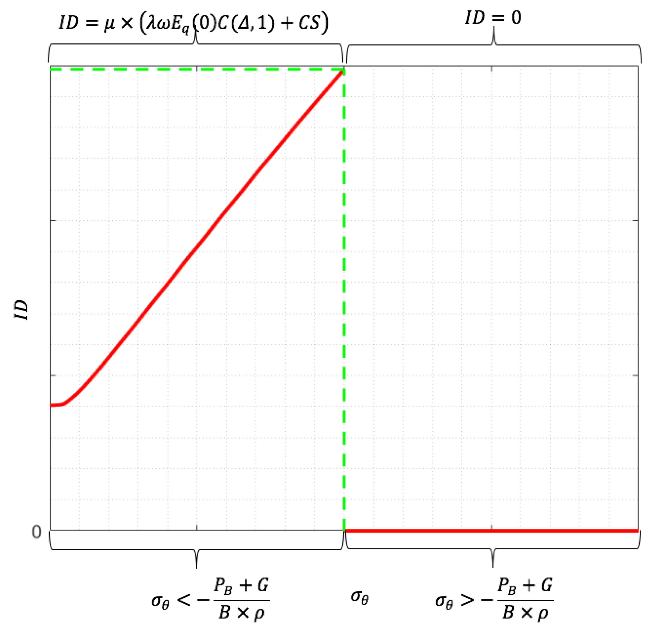
According to Corollary 4, we drew the entire function image of inside debt as shown in Figure 2. Figure 2 shows that, initially, inside debt value is positively associated with the default risk; however, this is not indefinite. After a point when σ θ = P B + G B × ρ , the bank goes bankrupt and inside debt changes to zero. We explain this phenomenon further in Section 4.4.
On the basis of Corollary 4, bankruptcy occurs when σ θ > P B + G B × ρ . This is consistent with Roy [43] and Laeven and Levine [44], who stated that insolvency is defined as a state in which losses surmount equity. □

4. Discussion

4.1. A Case Study: John G. Stumpf of Wells Fargo & Co.

4.1.1. Data

For calibrating the parameters of the cost functions introduced in Section 3, we used CEO compensation data and U.S. bank accounting data from the ExecuComp and BvD Orbis databases. Table 2 lists the annual compensation and other financial data for perhaps one of the most famous CEOs in American banking business, John G. Stumpf of Wells Fargo & Co.
The variables of the first six columns in Table 2 are related to the compensation received by John G. Stumpf, CEO of Wells Fargo & Co, between 26 June 2007 and 12 October 2016. We used the equity incentive plan, which is the value of unearned/unvested shares at the end of each fiscal year, as the approximation of inside equity value per year ( I E y ) . Inside debt value per year ( I D y ) represents present value of accumulated pension benefits from all pension plans. The total compensation value per year ( T C y ) in the background of Assumption 8 in this paper is the sum of cash salary ( C S y ) , inside equity value per year ( I E y ) , and inside debt value per year ( I D y ) , as reported by the ExecuComp database.
The last two columns in Table 2 are the calculated variables related to the financial situation of Wells Fargo & Co. ROE is ROE in the last available year; total equity value ( E q ( t ) ) is the total equity in the last available year, as shown in BvD Orbis—Global Financials for Banks (in USD).
All values are reported in millions of dollars as of December 31 of each year. Stumpf retired in October of 2016; thus, his compensation that year was not a full 12 months. The same applies for his starting year in 2007.

4.1.2. Calculation of Variables

The particular value of variables needed in 2015 were measured as follows.   σ θ of 2015 was inferred from the volatility of return on equity ( R O E ) , σ θ = 0.0737 . Total equity value ( E q ( t ) ) is assumed to total equity last available year, E q ( 0 ) = 171 , 567 , 000 . The risk-free rate r is the mean of one-month interest rates of national debt during November 2015 in the U.S., r = 0.07 .
The structure coefficient is as follows:
μ = I D C S + I E = 164842.9 26538.88 + 207031.465 0.7058
For Stumpf’s entire tenure,
κ = D a y   N u m   F r o m   20070626   t o   20161012 365 = 9 + 119 365 9.326
and inside debt frequency λ = 9 ,   Δ = κ λ = 1.036 .
The fraction of equity paid as inside equity is as follows:
ω = I E y ( y e a r   2015 ) λ × C ( Δ , 1 ) × A ( 0 ) = 34870.673 9 × C ( 1.036 , 1 ) × 171567000 0.000295
Stumpf’s compensation structure and holdings of inside debt are not exceptional. We investigated CEO pensions in the banking industry and found that the above patterns are generally present in the data. The rest of this section elaborates upon this finding.

4.2. Simulation Analysis

4.2.1. Significance of Fitting Maps

Figure 3, Figure 4 and Figure 5 verify the conclusion in Section 3. Since the inside debt function contains an option function and the option function is a multivariate implicit function, it is impossible to directly write the expression between the risk and the option price, but it can be drawn using the specific point method and MATLAB software (Harbin Institute of Technology, Harbin, China) to obtain the fitting map related to I D . From the fitting map, we obtained other information not directly determined from the equations.
Overall, the data in Figure 3, Figure 4 and Figure 5 were calculated in Section 4.1. The specific data used in the figure of the function image and the basis of the propositions or corollaries in this paper are introduced in the note below each figure.
Unexpectedly, we found that inside debt also has a negative effect on the sample banks’ risk reduction, as found for inside equity with Assumption 14 according to our model.

4.2.2. Analysis of Simulation Result

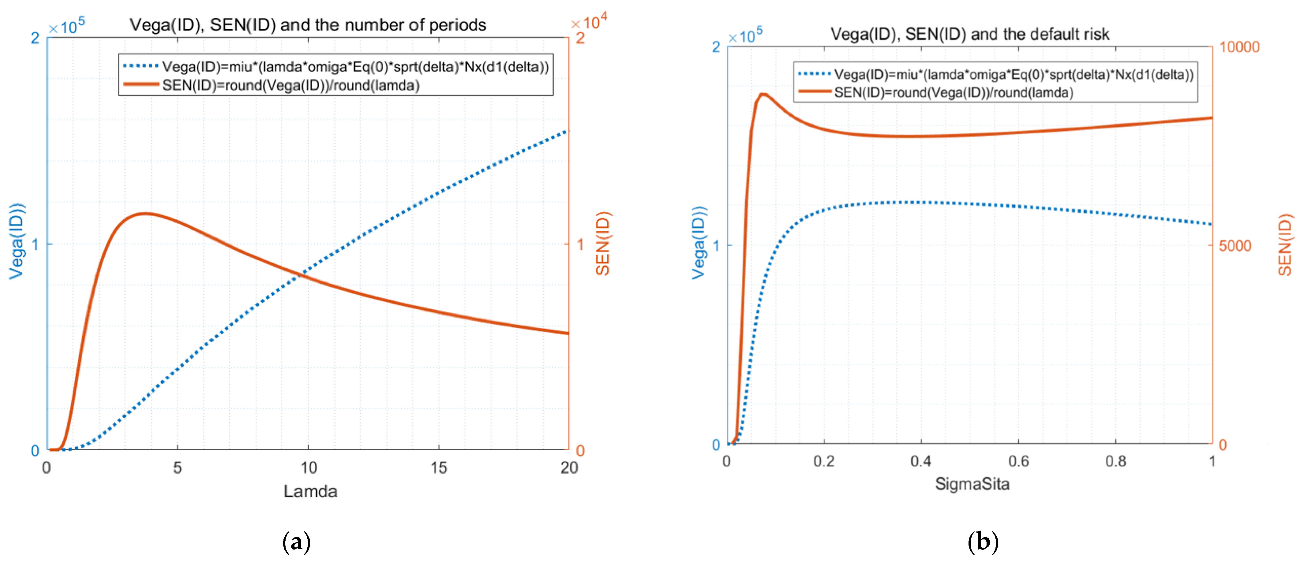
Figure 3a illustrates inside debt value ( I D ) and the corresponding risk-taking incentive ( V e g a I D ) with respect to the number of periods ( λ ) based on Proposition 1 and Corollary 2 for Wells Fargo & Co. The image of the inside debt was obtained by fitting the λ value to the corresponding I D value (Figure 3a, blue dotted line), and the image of the Vega of inside debt was directly drawn by Equation (40) (Figure 3a, orange-red solid line).
Figure 3b illustrates inside debt value ( I D ) and the corresponding risk-taking incentive ( V e g a I D ) with respect to the default risk ( σ θ ) based on Proposition 1 and Corollary 1 for the example bank. Similar to Figure 3a, the image of the inside debt was obtained by fitting the σ θ value to the corresponding I D value (Figure 3b, blue dotted line). The image of the Vega of inside debt was directly drawn using Equation (40) (Figure 3b, orange-red solid line).
The difference in the two figures is that the former assumes that the value of the default risk ( σ θ ) is constant ( σ θ = 0.0737 ) and that the latter assumes that the value of the number of periods ( λ ) is unchanged ( λ = 9 ) . The higher the number of λ , the shorter the inside debt time interval Δ if the banker’s tenure κ is unchanged. Figure 3a shows that both the inside debt value and the Vega of inside debt are positively corelated with the number of periods. Thus, from our model and the numerical example in Figure 3a, the higher the inside debt payment frequency, the higher the inside debt value and the stronger the risk-taking incentives.
Figure 3b shows that the inside debt value ( I D ) increases the earnings’ volatility ( σ θ ) ; when σ θ < 0.05 , this increase is not obvious or even negligible, but when σ θ is greater than 0.05, the two exhibit an approximately linear growth relationship, just like the call option function. As the default risk ( σ θ ) increases, the Vega value of inside debt first rapidly grows and then slowly falls back.
From another perspective, both number of periods ( λ ) and the default risk ( σ θ ) increase with the inside debt value ( I D ) . As a consequence, the shorter the time period Δ = κ / λ , the stronger the effect of default risk. This demonstrates that bankers with shorter tenure have a stronger incentive to take more risks for greater return. This is in agreement with Gopalan et al. (prediction 2), who concluded that the shorter the pay duration of a firm, the more volatile the cash flows [35].
Figure 4a depicts the function image of the risk-taking incentive ( V e g a I D ) and the corresponding sensitivity of inside debt ( S E N I D ) with respect to the number of periods ( λ ) based on Proposition 1 and Corollary 3 for Wells Fargo & Co. As shown in the figure, the image of V e g a I D was directly drawn using Equation (40) (blue dotted line) and the image of S E N I D was obtained using Equation (49) (solid red line). We drew the images of V e g a T C and S E N T C about the total compensation according to Equations (52) and (53) and obtained some similar properties. The difference is that the value of total compensation also depends on the size of μ , which is related to the compensation structure. Our next focus was the impact of different compensation structures on the default risk σ θ .
Figure 4b presents the function image of the risk-taking incentive ( V e g a I D ) and the corresponding sensitivity of inside debt ( S E N I D ) with respect to the default risk ( σ θ ) based on Proposition 1 and Corollary 3 for Wells Fargo & Co. Figure 4b is the same as Figure 4a.
As shown in Figure 4a, starting from the origin when the number of periods ( λ ) increases, the sensitivity of inside debt ( S E N I D ) increases significantly initially. When λ is five (according to the practical meaning, λ can only take a positive integer, whereas we drew the real range image only to better observe the trend and nature), S E N I D reaches a peak and then decreases at a relatively slower rate.
Figure 4b shows that, compared with the Vega value of inside debt ( V e g a I D ) , the first half of the change trend of the sensitivity of inside debt ( S E N I D ) is much steeper (faster growth) and the latter half is smaller and is inverted U-shaped (decrease first and then increase, while V e g a I D is still slowly falling) and that the highest peak of S E N I D was reached when σ θ was 0.07.
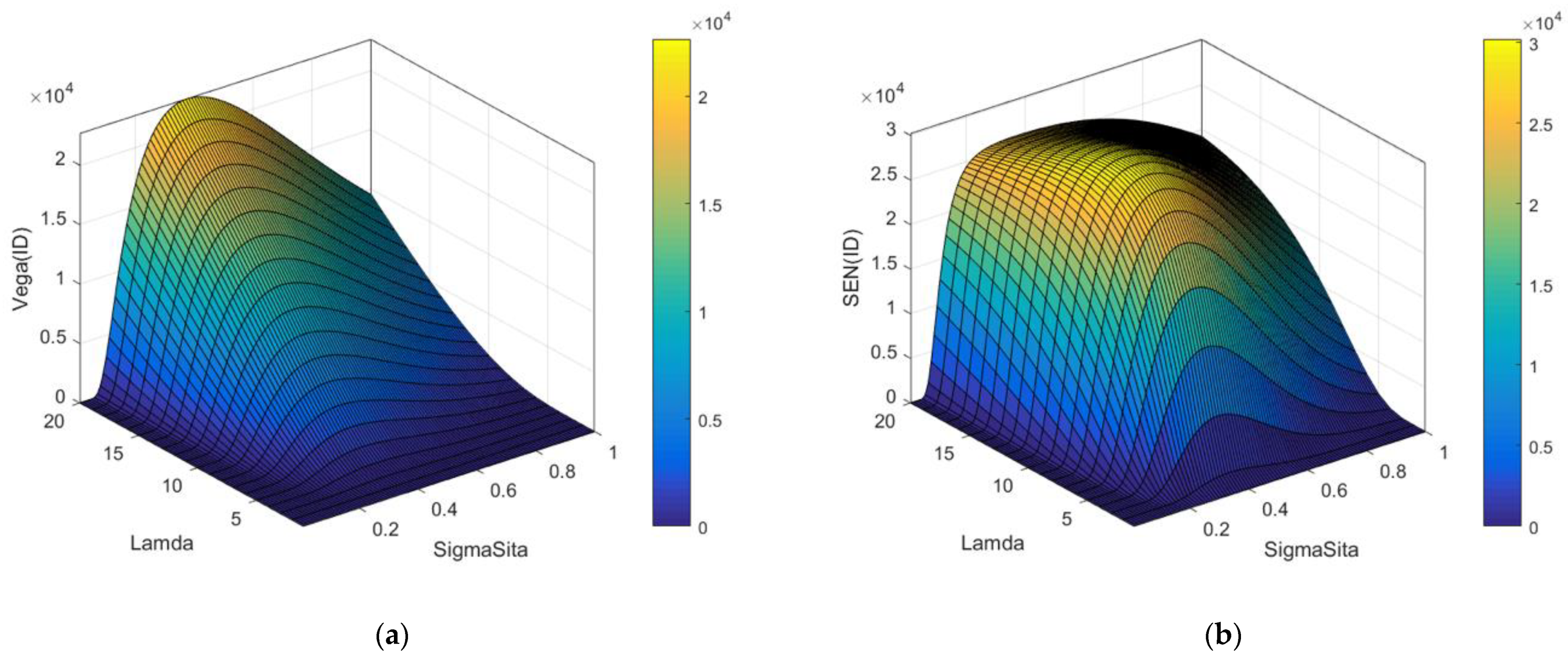
Figure 5a shows the three-dimensional image of risk-taking incentive ( V e g a I D ) and the corresponding number of periods ( λ ) and the default risk ( σ θ ) based on Proposition 1 and Corollary 2. Note that, for the parameter values for Wells Fargo & Co., we used the function in Equation (40) to draw this image. The color bar demonstrates the value of risk-taking incentive ( V e g a I D ) .
Figure 5 shows that, when λ increases, the influence of σ θ on ( I D ) also increases. However, when σ θ increases, the influence of λ on ( I D ) first increases and then decreases.
Figure 5b shows the three-dimensional image of the sensitivity of inside debt ( S E N I D ) and the corresponding number of periods ( λ ) and the default risk ( σ θ ) based on Proposition 1 and Corollary 3 for the example bank. We used the function in Equation (49) to draw this image. The color bar demonstrates the sensitivity of inside debt ( S E N I D ) .
A conclusion we drew from Figure 5b is that, as the number of periods ( λ ) increases, the change of effect of the default risk ( σ θ ) on the sensitivity of inside debt ( S E N I D ) is increasingly smaller especially when λ is larger than five.
To summarize, holding other variables unchanged, inside debt is positively correlated with the default risk. From Equations (10) and (12), inside debt value is calculated using a special method that overall characterizes the same monotonicity with the sum of inside equity and cash salary, although it is paid delayed. Under Assumption 14, executives inevitably take greater risks to obtain more inside debt in the future if it is possible for the bank to become bankrupt. This is not consistent with the traditional opinions. We clarify this question from a more comprehensive perspective in the following section.

4.3. Robustness

We used the data for Richard M. Adams, Sr. of United Bankshares to perform the robust test. He was the chairman and CEO of United Bankshares since 1 January 1984. His salary in 2006 was USD $641,667. The results showed that our conclusion is robust and effective. Under the precondition of Assumption 14, inside debt is positively associated with bank default risk and the number of periods is positively associated with bank default risk.

4.4. Black Box Effect

Initially, the term black box was the common name for electronic flight recorders, i.e., the instrument for recording aircraft flight and performance parameters. Black box also refers to a machine or process that we do not understand. Many things can be called black boxes in real life. For example, the computer is a black box to some people because they do not understand the internal workings of a computer. The same is true for other kinds of software. In traditional management terms, a black box is a device, system, or object that can only be viewed in terms of its input, output, and transfer characteristics without any knowledge of its internal workings [50]. Specifically, the meaning of black boxes in scholarly research is different and no uniform standard exists. For instance, Renmans et al. [51] used “opening the black box of performance-based financing in low- and lower-middle-income countries” to indicate they wanted to identify the unknown part about the exact mechanisms triggered by performance-based financing (PBF) arrangements. Brown et al. [52] aimed to penetrate the black box of sell-side financial analysts by providing new insights into the inputs that analysts use and the incentives they face.
In general, the common feature of black boxes is that, for a certain group, the person is not clear about the specific principle of the occurrence of this thing or event by only being able to observe the appearance of the thing (or only have the ability to use) or by only seeing the superficial phenomenon that has happened.
In this paper, black box specifically refers to the fact that bank executives are not clear. The risk will cause the bank to go bankrupt, which will occur suddenly, and they will know the bankruptcy, but the inherent law used to control the risk using specific indicators or precise scientific rules or methods is not clear. This phenomenon is called the black box effect of bankers.
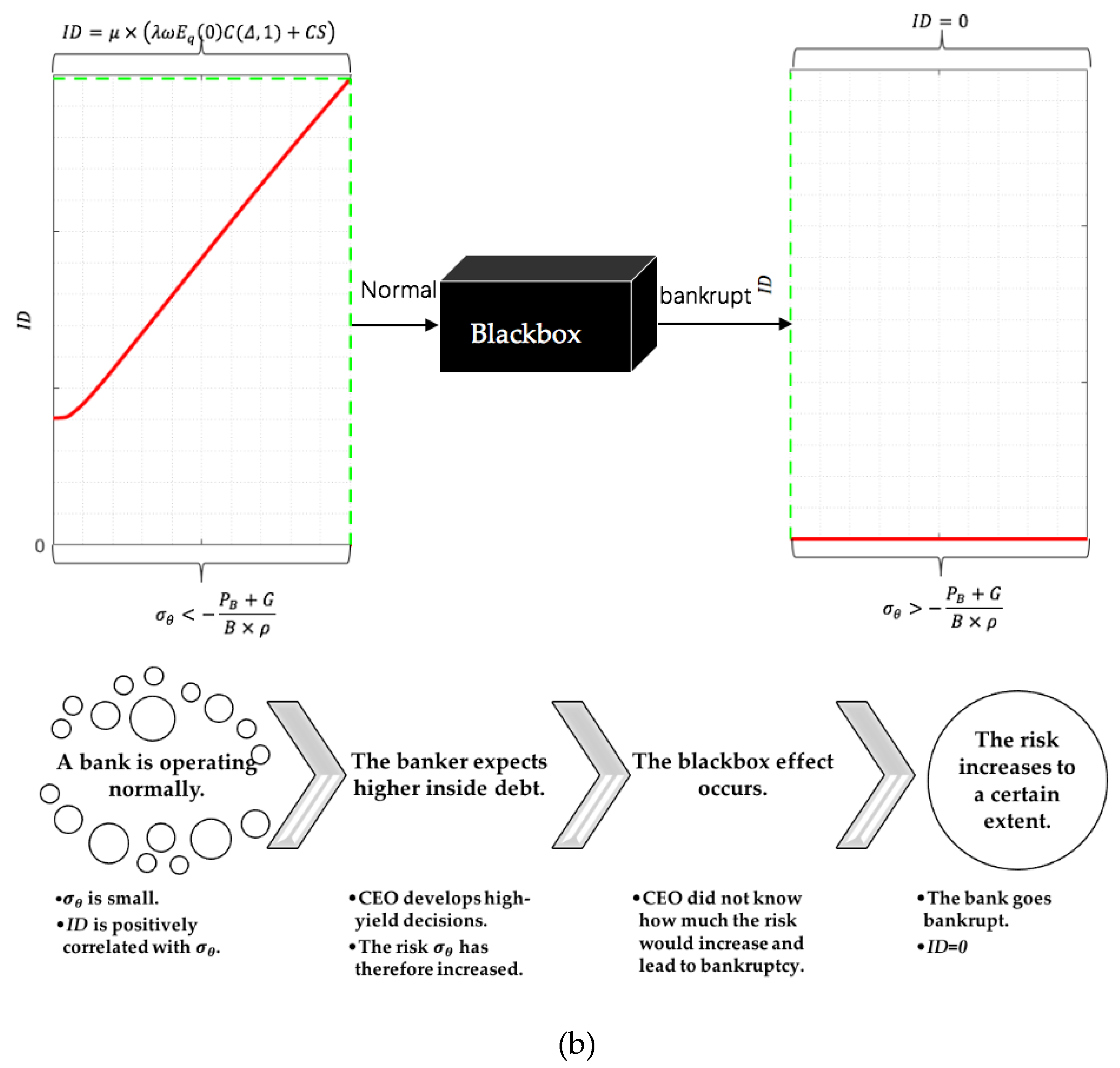
Specifically, assume a bank is operating normally with low default risk σ θ . As a consequence, based on Proposition 1 and Corollary 1, the value of inside debt is positively correlated with σ θ . Then, the banker expects higher inside debt value, so they make high-yield decisions. Therefore, σ θ increases. Due to not understanding the increased level of risk that would lead to bankruptcy, the black box effect occurs. If the risk increases to a certain level, the bank is bankrupt and no inside debt can be issued. A schematic diagram and the corresponding flow chart of the black box effect based on Corollary 4 are shown in Figure 6.
Corollary 4′.
Although I D increases by σ θ , when σ θ is beyond a particular level, bankruptcy occurs and I D suddenly drops to zero. This phenomenon is called the black box effect:
I D = { μ × ( λ ω E q ( 0 ) C ( Δ , 1 ) + C S )   i f   σ θ P B + G B × ρ 0   i f   σ θ > P B + G B × ρ
where μ = M S κ n = m a x ( 0 , R A ) K A p ( n ) ( 1 + d ) n , κ = S K + A = λ Δ , C ( Δ , 1 ) is the call option price from Equation (22), ω is the fraction of equity paid out as inside debt, E q ( 0 ) is the initial net asset value, σ θ is the volatility of R O E , P B is total profits unrelated to bad debts, G is good credit equity, B is poor credit equity, and ρ is the correlation coefficient between risk and bad debt.
Proof. 
On the basis of Corollary 4 and the definition of black box in our paper, we obtained the result. The key reason that leads to the production black box effect is that the banker is unable to identify the specific relationship between bank risk and bankruptcy. Banks are originally financial institutions that rely mainly on the issuance of loan profits, so credit risk is inevitable. No return is risk-free, and zero risk results in zero profit. Executives take risks in pursuit of higher future inside debt; conversely, executives worry that, if this kind of compensation (inside debt, different from inside equity and cash salary) is not paid in time, if the bank goes bankrupt, they will not receive the compensation. Therefore, the executives properly converge and control the risk level. However, they do not know how to calculate the best balance point and risk level. This is the significance of the black box effect. In other words, inside debt motivates executives to take more risks. However, they fear bankruptcy and restrain increases in risk to a certain extent. This is a complicated psychological process and situation. In our opinion, although the effect of inside debt on increase the risk is not as strong as inside equity, it is an inaccurate tool used for risk reduction. □

5. Conclusions

In this study, we modeled a banker’s long-term compensation, which has a linear relationship with a series of sequential call options on the bank’s return on equity, based on a practical calculation. We demonstrated the relationship of inside debt with the bank’s default risk by formulating a particular formula. Firstly, we examined this relationship but the bank’s possibility of bankruptcy was not considered, cash salary of bankers was paid per year and was irrelevant to the bank risk, and inside equity was paid per time (usually not by year) and was a series of sequential call options. Inside debt is paid in the latter part of the banker’s tenure and the calculation of inside debt is linearly related to the sum of cash salary and inside equity per year. Therefore, we defined the three kinds of compensation in three dimensions: inside debt per period, per year, and during the tenure, as well as for inside equity and cash salary for the convenience of calculation. After setting the model of inside debt and the default risk, we simulated the result using data from Wells Fargo & Co. to draw the function image to identify additional features. Then, considering the possibility of bankruptcy, we found a black box effect for the relationship of inside debt and bank default risk. In other words, inside debt motivates executives to take more risks. However, they fear bankruptcy and restrain the risk increase to a certain extent. This is a complicated psychological process and situation. Therefore, pay me later reduces the risk, which is different than reported by Sundaram et al. [2], whose opinion was that pay me later is positively related with the distance to bankruptcy, which is good for risk reduction. Bankers with shorter tenure are strongly incentivized to take more risks for greater return of inside debt. In reality, inside equity is issued on a recurring basis only when the company’s equity increases and inside debt is deferred, the value of which is linearly related to the first two.
For the first time, we defined and distinguished the three types of compensation calculations and the relationship with risk in the three dimensions and further analyzed the changes in their nature when considering bankruptcy. For the first time, we established an executive’s tenure as a term in this relationship. This long-term compensation model lays the foundation for further theoretical analysis because, in prior studies, most researchers only used annual data to analyze the relationship of different kinds of executive compensation and bank risk and ignored the compensation of one CEO for their entire tenure. In other words, we set up a long-term compensation model, which provides a new perspective for theoretical analysis. The shortcoming of our study is that, although the compensation model is long term, due to information disclosure and other reasons, it does not consider other types of debt-based compensation such as long-term vesting schedules of equity awards and deferred compensation. We will focus on the factors affecting the compensation structure μ and the impact of the compensation structure on the risk based on Equation (18).

Author Contributions

Conceptualization, T.M. and M.J.; methodology, T.M.; software, T.M.; validation, T.M., M.J. and X.Y.; formal analysis, T.M.; investigation, T.M.; resources, T.M.; data curation, T.M.; writing—original draft preparation, T.M.; writing—review and editing, T.M., M.J., and X.Y.; visualization, T.M.; supervision, M.J.; project administration, X.Y.; funding acquisition, M.J. All authors have read and agreed to the published version of the manuscript.

Funding

This research was funded by the National Natural Science Foundation of China, grant number 71502044, and the China Postdoctoral Science Foundation, grant number 2015M570300.

Acknowledgments

We acknowledge Fu Zhenwu of Harbin Institute of Technology for the given help about the software MATLAB.

Conflicts of Interest

The authors declare no conflict of interest.

Appendix A

Table A1. Main conclusions of this paper.
PreconditionClassificationKinds of CompensationLong Term ModelAnnual ModelModel of Each TimeRelationship with Risk
From Predecessors or IntuitionFrom Theoretical AnalysisFrom Simulation ResultsCorresponding Figure
(A) When Assumption 14 is established, i.e.,
Lemma 1′:
σ θ P B + G B × ρ  
Structure   ( μ )
μ = M S κ × n K A p ( n ) ( 1 + d ) n
where   n = m a x ( 0 , R A ) .
(a) Cash Salary constant   C S C S y = C S κ C S t = C S κ irrelevant ( C S ) σ θ = 0 irrelevanta horizontal straight line across the origin
(b) Inside equity I E = λ ω E q ( 0 ) C ( Δ , 1 ) I E y = ω Δ E q ( 0 ) C ( Δ , 1 ) I E t = ω E q ( 0 ) C ( Δ , 1 ) ( + ) ( I E ) σ θ > 0 ( + ) * analogous to Figure 3
(c) Inside debtProposition 1:
I D = μ × ( λ ω E q ( 0 ) C ( Δ , 1 ) + C S )
I D y = μ × ( ω Δ E q ( 0 ) C ( Δ , 1 ) + C S y ) I D t = μ × ( ω E q ( 0 ) C ( Δ , 1 ) + C S t ) ( ) Corollary 1:
( I D ) σ θ > 0
( + ) * Figure 3
Pay contract(d) Total compensationProposition 1′:
T C = ( 1 + μ ) ( λ ω E q ( 0 ) C ( Δ , 1 ) + C S )
T C y = ( 1 + μ ) × ( ω Δ E q ( 0 ) C ( Δ , 1 ) + C S y ) T C t = ( 1 + μ ) × ( ω E q ( 0 ) C ( Δ , 1 ) + C S t ) ( ? ) ( T C ) σ θ > 0 ( + ) * analogous to Figure 3
Other Relative Variables(e) Vega V e g a I D = I D σ θ = μ λ ω E q ( 0 ) e x p ( r Δ ) Δ N x ( d 2 ( Δ ) )
V e g a T C = ( 1 + μ ) λ ω E q ( 0 ) e x p ( r Δ ) Δ N x ( d 2 ( Δ ) )
( ? ) Corollary 2:
I D λ + 1 I D λ
( + ) * Figure 3 and Figure 5
(f) Sensitivity S E N I D = 2 ( I D ) σ θ λ = μ ω E q ( 0 ) Δ 8 σ θ 2 ( 4 r 2 Δ + 4 σ θ 2 + 4 r Δ σ θ 2 + Δ σ θ 4 ) N x ( d 1 ( Δ ) )
S E N T C = ( 1 + μ ) ω E q ( 0 ) Δ 8 σ θ 2 ( 4 r 2 Δ + 4 σ θ 2 + 4 r Δ σ θ 2 + Δ σ θ 4 ) N x ( d 1 ( Δ ) )
( ? ) Corollary 3:
( I D λ + 1 ) σ θ ( I D λ ) σ θ
( + ) * Figure 4 and Figure 5
(B) Taking Lemma 1
( σ θ > P B + G B × ρ ) into consideration, i.e., containing the possibility of bankruptcy
The black box effectInside debtCorollary 4:
I D = { μ × ( λ ω E q ( 0 ) C ( Δ , 1 ) + C S )   i f   σ θ P B + G B × ρ 0   i f   σ θ > P B + G B × ρ
( ) a conflict situation ( + )   and   ( ) Figure 2
Variables (a), (b) and (d) in precondition (A)Being similar to Corollary 4, we can write the formula in the following template:
( a ) , ( b )   a n d   ( d ) = { f o r m u l a   i n   ( A )   i f   σ θ P B + G B × ρ 0   i f   σ θ > P B + G B × ρ
like above
(irrelevant/ +/?)
a conflict situation ( + )   and   ( ) analogous to Figure 2
Note: ( + ) stands for a positive relationship between the two variables, ( + ) * stands for the positive relationship that is only established on behalf of Assumption 14 (if containing the possibility of bankruptcy, see Proposition 1′ and Corollary 4 in Section 3.5the black box effect), ( ) stands for the negative one, and ( ? ) stands for the unknown one.

References

  1. Jensen, M.C.; William, H.M. Theory of the firm: Managerial behavior, agency cost, and ownership structure. J. Financ. Econ. 1976, 3, 305–360. [Google Scholar] [CrossRef]
  2. Sundaram, P.K.; Yermack, D.L. Pay me later: Inside debt and its role in managerial compensation. J. Financ. 2007, 62, 1551–1588. [Google Scholar] [CrossRef] [Green Version]
  3. Abad-Segura, E.; Cortés-García, F.J.; Belmonte-Ureña, L.J. The Sustainable Approach to Corporate Social Responsibility: A Global Analysis and Future Trends. Sustainability 2019, 11, 5382. [Google Scholar] [CrossRef] [Green Version]
  4. Becht, M.; Bolton, P.; Roell, A. Why bank governance is different. Oxf. Rev. Econ. Policy 2012, 27, 437–463. [Google Scholar] [CrossRef] [Green Version]
  5. Beltratti, A.; Stulz, R.M. The credit crisis around the globe: Why did some banks perform better? J. Financ. Econ. 2012, 105, 1–17. [Google Scholar] [CrossRef]
  6. Erkens, D.H.; Hung, M.; Matos, P. Corporate governance in the 2007–2008 financial crisis: Evidence from financial institutions worldwide. J. Corp. Financ. 2012, 18, 389–411. [Google Scholar] [CrossRef]
  7. Berger, A.N.; Kick, T.; Schaeck, K. Executive board composition and bank risk taking. J. Corp. Financ. 2014, 28, 48–65. [Google Scholar] [CrossRef]
  8. Minton, B.A.; Taillard, J.P.; Williamson, R. Financial expertise of the board, risk taking, and performance: Evidence from bank holding companies. J. Financ. Quant. Anal. 2014, 49, 351–380. [Google Scholar] [CrossRef]
  9. International Monetary Fund. Risk-taking by banks: The role of governance and executive pay. In Global Financial Stability Report: Risk-Taking, Liquidity, and Shadow Banking: Curbing Excess while Promoting Growth; IMF: Washington, DC, USA, 2014. [Google Scholar]
  10. Hagendorff, J.; Vallascas, F. CEO pay incentives and risk taking: Evidence from bank acquisitions. J. Corp. Financ. 2011, 17, 1078–1095. [Google Scholar] [CrossRef]
  11. DeYoung, R.; Peng, E.Y.; Yan, M. Executive compensation and business policy choices at US commercial banks. J. Financ. Quant. Anal. 2013, 48, 165–196. [Google Scholar] [CrossRef]
  12. Galletta, S.; Mazzù, S. Liquidity Risk Drivers and Bank Business Models. Risks 2019, 7, 89. [Google Scholar] [CrossRef] [Green Version]
  13. Bennett, R.L.; Guntay, L.; Unal, H. Inside debt, bank default risk and performance during the crisis. J. Financ. Intermed. 2015, 24, 487–513. [Google Scholar] [CrossRef]
  14. Van Bekkum, S. Inside debt and bank risk. J. Financ. Quant. Anal. 2015, 51, 359–385. [Google Scholar] [CrossRef]
  15. Bolton, P.; Mehran, H.; Shapiro, J. Executive compensation and risk taking. Rev. Financ. 2015, 19, 2139–2181. [Google Scholar] [CrossRef]
  16. Cheng, I.H.; Hong, H.; Scheinkman, J.A. Yesterday’s heroes: Compensation and risk at financial firms. J. Financ. 2015, 70, 839–879. [Google Scholar] [CrossRef]
  17. Keys, B.J.; Mukherjee, T.; Seru, A.; Vig, V. Financial regulation and securitization: Evidence from subprime loans. J. Monet. Econ. 2009, 56, 700–720. [Google Scholar] [CrossRef]
  18. Fahlenbrach, R.; Prilmeier, R.; Stulz, R.M. This time is the same: Using bank performance in 1998 to explain bank performance during the recent financial crisis. J. Financ. 2012, 67, 2139–2185. [Google Scholar] [CrossRef]
  19. Ellul, A.; Yerramilli, V. Stronger risk controls, lower risk: Evidence from US bank holding companies. J. Financ. 2013, 68, 1757–1803. [Google Scholar] [CrossRef] [Green Version]
  20. Köhler, M. Which banks are more risky? The impact of business models on bank stability. J. Financ. Stab. 2015, 16, 195–212. [Google Scholar] [CrossRef]
  21. Wu, T.H.; Lin, M.C. Relationship of CEO inside debt and corporate social performance: A data envelopment analysis approach. Financ. Res. Lett. 2019, 29, 308–314. [Google Scholar] [CrossRef]
  22. Srivastav, A.; Armitage, S.; Hagendorff, J. CEO inside debt holdings and risk-shifting: Evidence from bank payout policies. J. Bank Financ. 2014, 47, 41–53. [Google Scholar] [CrossRef] [Green Version]
  23. Srivastav, A.; Armitage, S.; Hagendorff, J.; King, T. Better safe than sorry? CEO inside debt and risk-taking in bank acquisitions. J. Financ. Stab. 2018, 36, 208–224. [Google Scholar] [CrossRef]
  24. Reid, C.D. CEO retirement compensation: Is inside debt excess compensation or a risk management tool? Bus. Horiz. 2018, 61, 721–731. [Google Scholar] [CrossRef]
  25. Mo, K.; Kim, Y.J.; Park, K.J. Chief Executive Officer Inside Debt Holdings and Labor Investment Efficiency. Asia Pac. J. Financ. Stud. 2019, 48, 476–502. [Google Scholar] [CrossRef]
  26. Milidonis, A.; Nishikawa, T.; Shim, J. CEO Inside Debt and Risk Taking: Evidence from Property-Liability Insurance Firms. J. Risk Insur. 2019, 86, 451–477. [Google Scholar] [CrossRef]
  27. Deng, K.; He, J.; Kong, D.; Zhang, J. Does inside debt alleviate banks’ risk taking? Evidence from a quasi-natural experiment in the Chinese banking industry. Emerg. Mark. Rev. 2019, 40, 100622. [Google Scholar] [CrossRef]
  28. Chen, L.; Fan, H. CEO inside debt and bank loan syndicate structure. Rev. Financ. Econ. 2017, 34, 74–85. [Google Scholar] [CrossRef]
  29. Bhandari, A.; Mammadov, B.; Thevenot, M. The impact of executive inside debt on sell-side financial analyst forecast characteristics. Rev. Quant. Financ. Account. 2018, 51, 283–315. [Google Scholar] [CrossRef]
  30. Sheikh, S. CEO inside debt, market competition and corporate risk taking. Int. J. Manag. Financ. 2019, 15, 636–657. [Google Scholar] [CrossRef]
  31. Li, Z.F.; Lin, S.; Sun, S.; Tucker, A. Risk-adjusted inside debt. Glob. Financ. J. 2018, 35, 12–42. [Google Scholar] [CrossRef] [Green Version]
  32. Li, Y.; Zhang, X.-Y. Impact of board gender composition on corporate debt maturity structures. Eur. Financ. Manag. 2019, 25, 1286–1320. [Google Scholar] [CrossRef]
  33. Li, W.-H.; Rhee, S.G.; Shen, C.H. CEO inside debt and convertible bonds. J. Bus. Financ. Account. 2018, 45, 232–249. [Google Scholar] [CrossRef]
  34. Im, H.-K.; Choi, S.; Hwang, I. CEO Inside Debt and Asymmetric Cost Behavior. Korea Account. Rev. 2018, 43, 51–88. [Google Scholar] [CrossRef]
  35. Freund, S.; Latif, S.; Phan, H.V. Executive compensation and corporate financing policies: Evidence from CEO inside debt. J. Corp. Financ. 2018, 50, 484–504. [Google Scholar] [CrossRef]
  36. Dasgupta, S.; Lin, Y.; Yamada, T.; Zhang, Z. Employee Inside Debt and Firm Risk-Taking: Evidence from Employee Deposit Programs in Japan. Rev. Corp. Financ. Stud. 2019, 8, 302–347. [Google Scholar] [CrossRef]
  37. Colonnello, S.; Curatola, G.; Hoang, N.G. Direct and indirect risk-taking incentives of inside debt. J. Corp. Financ. 2017, 45, 428–466. [Google Scholar] [CrossRef] [Green Version]
  38. Chi, S.; Huang, S.X.; Sanchez, J.M. CEO Inside Debt Incentives and Corporate Tax Sheltering. J. Account. Res. 2017, 55, 837–876. [Google Scholar] [CrossRef]
  39. Brisker, E.R.; Wang, W. CEO’s Inside Debt and Dynamics of Capital Structure. Financ. Manag. 2017, 46, 655–685. [Google Scholar] [CrossRef]
  40. Belkhir, M.; Boubaker, S.; Chebbi, K. CEO inside debt and the value of excess cash. J. Appl. Account. Res. 2018, 19, 225–244. [Google Scholar] [CrossRef]
  41. Beavers, R. CEO inside debt and firm debt. Corp. Gov. Int. J. Bus. Soc. 2018, 18, 686–713. [Google Scholar] [CrossRef]
  42. Black, F.; Scholes, M. The Pricing of Options and Corporate Liabilities. J. Polit. Econ. 1973, 81, 637–654. [Google Scholar] [CrossRef] [Green Version]
  43. Roy, A.D. Safety first and the holding of assets. Econometrica 1952, 20, 431–449. [Google Scholar] [CrossRef]
  44. Laeven, L.; Levine, R. Bank governance, regulation and risk taking. J. Financ. Econ. 2009, 93, 259–275. [Google Scholar] [CrossRef] [Green Version]
  45. Kaplan, E.L.; Meier, P. Nonparametric estimation from incomplete observations. J. Am. Stat. Assoc. 1958, 53, 456–481. [Google Scholar] [CrossRef]
  46. Robert, C. Merton. On the Pricing of Corporate Debt: The Risk Structure of Interests Rates. J. Financ. 1974, 29, 449–470. [Google Scholar]
  47. Jokivuolle, E.; Keppo, J.; Yuan, X. Bonus Caps, Deferrals and Bankers’ Risk-Taking. Manag. Sci. under review.
  48. Boyle, P.P.; Scott, W.R. Executive Stock Options and Concavity of the Option Price. J. Deriv. 2006, 13, 72–84. [Google Scholar] [CrossRef]
  49. Gopalan, R.; Milbourn, T.; Song, F.; Thakor, A.V. The Optimal Duration of Executive Compensation: Theory and Evidence. AFA 2012 Chicago Meetings Paper. Available online: http://ssrn.com/abstract=1656603 (accessed on 10 November 2019).
  50. Wikidata. Available online: https://www.wikidata.org/wiki/Q29256 (accessed on 18 November 2019).
  51. Renmans, D.H.; Holvoet, N.O.; Orach, C.G.; Criel, B. Opening the ‘black box’ of performance-based financing in low- and lower middle-income countries: A review of the literature. Health Policy Plan. 2016, 31, 1297–1309. [Google Scholar] [CrossRef] [PubMed] [Green Version]
  52. Brown, L.D.; Call, A.C.; Clement, M.B.; Sharp, N.Y. Inside the “Black Box” of Sell-Side Financial Analysts. J. Account. Res. 2015, 53, 1–47. [Google Scholar] [CrossRef]
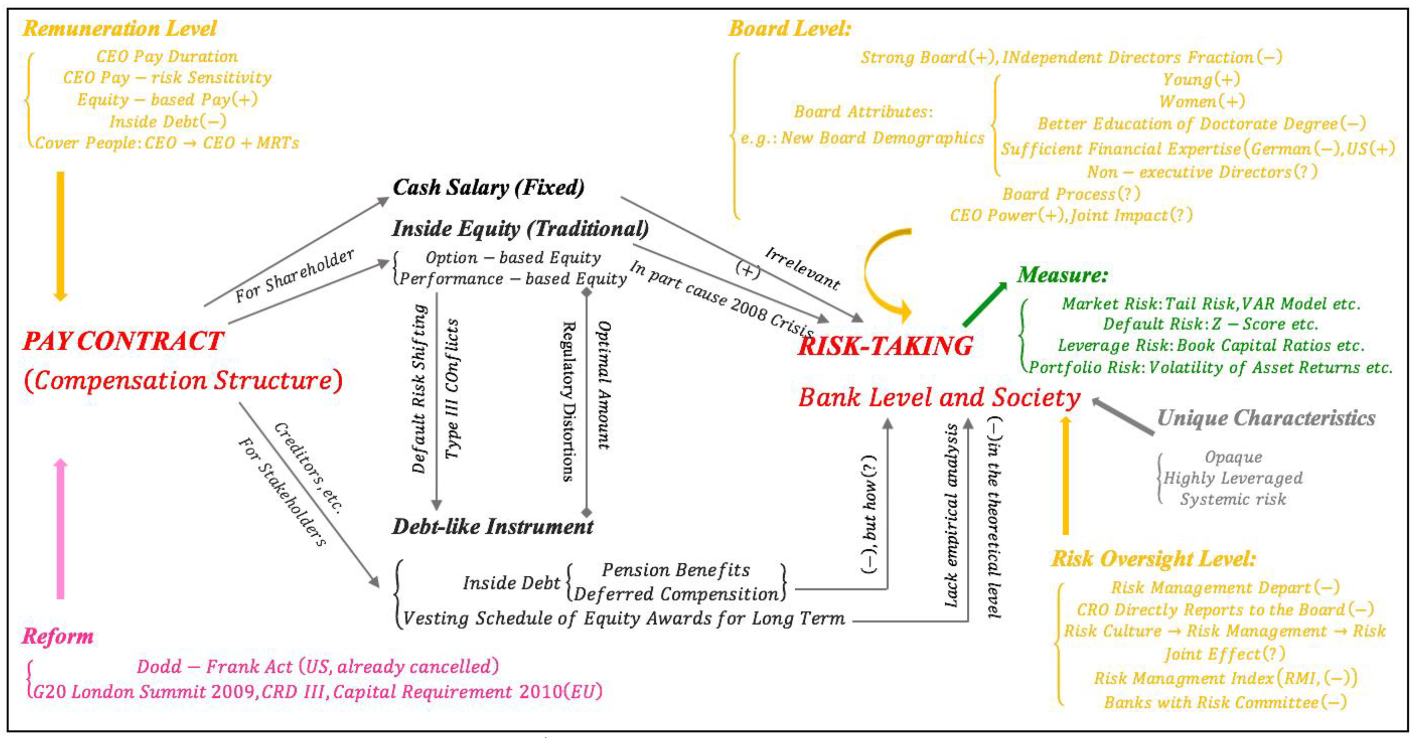
Figure 1. Summary of related studies. (Note: ( + ) stands for a positive relationship between the two variables, ( ) stands for the negative one, and ( ? ) stands for the unknown one.).
Sustainability 12 00035 g001
Figure 2. Schematic diagram of inside debt value ( I D ) and the corresponding default risk ( σ θ ) based on Corollary 4 in the more comprehensive situation of taking the probability of bankruptcy during the term of the executive (when Assumption 14 is invalid). (Note: Parameter values of the left half of the image are on behalf of Lemma 1′. (example bank: Wells Fargo & Co, year: 2015): E q ( 0 ) = 171567000 ,   r = 0.07 ,   μ = 0.7058 , κ = 9.326 ,   ω = 0.000295 ,   a n d   λ = 9 . The risk-free rate r is the mean of the 1-month interest rate of national debt during November 2015 in the US.)
Sustainability 12 00035 g002
Figure 3. (a) Fitting map of inside debt value ( I D ) and the corresponding risk-taking incentive ( V e g a I D ) with respect to the number of periods ( λ ) based on Proposition 1 and Corollary 2; (Note: Parameter values (example bank: Wells Fargo & Co, year: 2015): E q ( 0 ) = 171567000 , σ θ = 0.0737 ,   r = 0.07 ,   μ = 0.7058 , κ = 9.326 ,   a n d   ω = 0.000295 . The risk-free rate r is the mean of the 1-month interest rate of national debt during November 2015 in the US.) (b) Fitting map of inside debt value ( I D ) and the corresponding risk-taking incentive ( V e g a I D ) with respect to the default risk ( σ θ ) based on Proposition 1 and Corollary 1. (Note: Parameter values (example bank: Wells Fargo & Co, year: 2015): E q ( 0 ) = 171567000 ,   r = 0.07 ,   μ = 0.7058 , κ = 9.326 ,   ω = 0.000295 ,   a n d   λ = 9 . The risk-free rate r is the mean of 1-month interest rate of national debt during November 2015 in the US.)
Sustainability 12 00035 g003
Figure 4. (a) Function image of the risk-taking incentive ( V e g a I D ) and the corresponding sensitivity of inside debt ( S E N I D ) with respect to the number of periods ( λ ) based on Proposition 1 and Corollary 3. (Note: Parameter values (example bank: Wells Fargo & Co, year: 2015): E q ( 0 ) = 171567000 , σ θ = 0.0737 ,   r = 0.07 , μ = 0.7058 ,   κ = 9.326 ,   a n d   ω = 0.000295 . The risk-free rate r is the mean of the 1-month interest rate of national debt during November 2015 in the US.) (b) Function image of the risk-taking incentive ( V e g a I D ) and the corresponding sensitivity of inside debt ( S E N I D ) with respect to the default risk ( σ θ ) based on Proposition 1 and Corollary 3. (Note: Parameter values (example bank: Wells Fargo & Co, year: 2015): E q ( 0 ) = 171567000 ,   r = 0.07 ,   μ = 0.7058 , κ = 9.326 ,   ω = 0.000295 ,   a n d   λ = 9 . The risk-free rate r is the mean of the 1-month interest rate of national debt during November 2015 in the US.)
Sustainability 12 00035 g004
Figure 5. (a) Three-dimensional image of risk-taking incentive ( V e g a I D ) and the corresponding number of periods ( λ ) and the default risk ( σ θ ) based on Proposition 1 and Corollary 2. (Note: Parameter values (example bank: Wells Fargo & Co, year: 2015): E q ( 0 ) = 171567000 , σ θ = 0.0737 ,   r = 0.07 ,   μ = 0.7058 , κ = 9.326 ,   a n d   ω = 0.000295 . The risk-free rate r is the mean of the 1-month interest rate of national debt during November 2015 in the US. The color bar demonstrates the value of I D .) (b) Three-dimensional image of sensitivity of inside debt ( S E N I D ) and the corresponding number of periods ( λ ) and the default risk ( σ θ ) based on Proposition 1 and Corollary 3. (Note: Parameter values (example bank: Wells Fargo & Co, year: 2015): E q ( 0 ) = 171567000 ,   r = 0.07 ,   μ = 0.7058 , κ = 9.326 ,   ω = 0.000295 ,   a n d   λ = 9 . The risk-free rate r is the mean of the 1-month interest rate of national debt during November 2015 in the US. The color bar demonstrates the value of σ θ .
Sustainability 12 00035 g005
Figure 6. (a) Schematic diagram of the black box in traditional views. (Note: Figure resource: Wikidata [50].) (b) Schematic diagram of the black box effect and the corresponding flow chart of the black box effect based on Corollary 4. (Note: The upper left half of the image (on behalf of Lemma 1′) is the fitting map of inside debt value ( ID ) with respect to the earnings volatility ( σ θ ) based on Proposition 1. Parameter values (example bank: Wells Fargo & Co, year: 2015): E q ( 0 ) = 171567000 ,   r = 0.07 , μ = 0.7058 , κ = 9.326 ,   ω = 0.000295 ,   a n d   λ = 9 . The risk-free rate r is the mean of the 1-month interest rate of national debt during November 2015 in the US. The upper right half of the image (on behalf of Lemma 1) is the fitting map of inside debt value ( I D ) with respect to the earnings volatility ( σ θ ) based on Corollary 4. The lower part of the picture is the flow chart corresponding to the upper part according to Corollary 4’.)
Sustainability 12 00035 g006aSustainability 12 00035 g006b
Table 1. Notations and definitions in theoretical analysis.
ClassificationNotationsDefinitionNotationsDefinitionNotationsDefinitionNotationsDefinition
Bankruptcy E the bank equity G good credit equityBpoor credit equity (negative) p ( b ) probability of bad debts
P B total profits not related to bad debts ρ correlation coefficient between risk and bad debt R O E return on equity σ θ volatility of ROE
Cash salary C S cash salary during banker’s tenure C S y cash salary per year C S t cash salary per time κ / k a p p a the executive’s tenure
Inside debt I D inside debt during banker’s tenure I D y inside debt per year I D t inside debt per time R the minimum retirement age
A the CEO’s current age p ( n ) the probability that one is alive n years d the firm’s cost of long-term debt K the terminal year of the pension
C t k cash salary and inside equity for year t P a number of past years M a multiplier factor S the executive’s number of working years
Inside equity I E inside equity during banker’s tenure I E y inside equity per year I E t inside equity per time r the risk-free rate
ω the fraction of equity λ the inside equity and inside debt frequency Δ the time interval C ( Δ ,   K C ) BS call option price
K C strike price of the call option   E q ( i Δ ) the bank equity N x ( x ) standard cumulative normal distribution n x ( x ) standard normal density
Compensation T C total compensation during banker’s tenure T C y total compensation per year T C t total compensation per time μ coefficient of compensation structure
Related measure V e g a I D Vega of inside debt S E N I D the sensitivity of inside debt V e g a T C Vega of total compensation S E N T C sensitivity of total compensation
Note: The notation E in classification bankruptcy and E q ( i Δ ) in inside equity are both the bank equity.
Table 2. John G. Stumpf’s compensation as CEO of Wells Fargo & Co ($).
YearAgeCash Salary per Year ( C S y ) Inside Debt Value per Year ( I D y ) Inside Equity Value per Year ( I E y ) * Total Compensation Value per Year ( T C y ) Return on Equity ( R O E ) Total Equity Value ( E q ( t ) )
200753749.61510,334.11011,083.720.244347,432,000
200854878.9210,061.95010,940.870.032470,949,000
200955560012,646.33028,491.730.1574105,846,000
2010563239.84714,051.6610,245.40441,604.930.1486119,155,000
201157280015,979.9624,313.42251,497.130.167130,189,000
201258280019,538.0432,717.16864,298.740.1792145,953,000
201359280018,744.9341,960.70156,481.340.1908154,646,000
201460280020,853.0934,936.41658,523.760.1829166,075,000
201561280019,972.5834,870.67350,760.2617.35171,567,000
2016622070.49822,660.327,987.68124,730.816.02175,820,000
Sum C S = 26,538.88 I D = 164,842.9 I E = 207,031.465 T C = 398,413.3
Note: To simplify the calculation, we choose the value of 2015, which is shaded grey in the table. ( I E y ) * is different every year in the table, but it does not contradict our model because, in our model, inside equity is paid by times and. on the basis of the increase of bank’s net asset, we denote I E y as inside equity per year only for easy distinction and calculation. The same is done for I D y .