Article

The Development Simulation of Urban Green Space System Layout Based on the Land Use Scenario: A Case Study of Xuchang City, China

1
College of Landscape Architecture, Nanjing Forestry University, Nanjing 210037, China
2
Shanghai Academy of Landscape Architecture Science and Planning, Shanghai 200232, China
*
Authors to whom correspondence should be addressed.
Sustainability 2020, 12(1), 326; https://doi.org/10.3390/su12010326
Submission received: 18 November 2019 / Revised: 21 December 2019 / Accepted: 27 December 2019 / Published: 31 December 2019
(This article belongs to the Section Sustainable Urban and Rural Development)

Abstract

:
The development and evolution of an urban green space system is affected by both natural effects and human intervention. The simulation and prediction of an urban green space system can enhance the foresight of urban planning. In this study, several land use change scenarios of the main urban area of Xuchang City were simulated from 2014 to 2030 based on high-resolution land use data. The layout of each scenario was evaluated using landscape indexes. A Cellular Automata–based method (i.e., future land use simulation, FLUS) was applied to develop the urban green space system, which we combined with urban land use evolution. Using recent data, the FLUS model effectively dealt with the uncertainty and complexity of various land use types under natural and human effects and solved the dependence and error transmission of multiperiod data in the traditional land use simulation process. The root mean square error (RMSE) of probability of the suitability occurrence module and the Kappa coefficient of the overall model simulation accuracy verification index both met accuracy requirements. It was feasible to combine the evolution of the urban green space system with urban land development. Moreover, under the Baseline Scenario, the urban land use layout was relatively scattered, and the urban green space system showed a disordered development trend. The Master Plan Scenario had a compact urban land use layout, and the green space system was characterized by networking and systematization, but it did not consider the service capacity of the green space. The Planning Guidance Scenario introduced constraint conditions (i.e., a spatial development strategy, green space accessibility, and ecological sensitivity), which provided a more intensive and efficient urban space and improved the service function of the green space system layout. Managers and planners can evaluate the urban future land use development mode under different constraints. Moreover, they would be able to adjust the urban planning in the implementation process. This work has transformed the technical nature of the planning work from “static results” to a “dynamic process”.

1. Introduction

In 2015, the United Nations presented seventeen sustainable development goals, three of which were closely related to urban green space: sustainable cities and communities, climate action, and life on land. An urban green space system serves multiple functions, including improving the urban living environment, human health, and well-being, adjusting the urban climate, maintaining the urban ecological biodiversity, and promoting urban sustainable development [1,2,3,4]. Urban green space system planning guides development, establishes layouts, and manages and controls the urban green space [5,6]. Traditional urban spatial planning work is mainly a spatial expression of the subjective needs and planning intentions of the government and planners; the requirements of urban residents have often not been considered [7,8,9]. One issue in planning is the uncertainty of the benefits game [10]. Urban green space system planning often lags behind urban master planning and often does not consider the coexistence and connection of various land use classification systems. As a result, urban green space system planning can be particularly passive and negative [11,12]. At present, due to rapid urbanization, the demands of the natural environment and the development intensity of various types of urban land use are rapidly changing. In the past, the planning mode of an “ultimate blueprint” (i.e., the control index based on a plot) was too rigid to respond to the future development scenario of a city in a timely manner. This led to contradictions between planning objectives and actual development demand [13].
A city is an open, complex, giant system [14,15]. As a subsystem of the city, the urban green space system is an important means for the development and evolution of the natural spatial elements of an urban area. The evolution of the urban green space system is not a simple bottom-up self-organization process. The construction of urban green space usually is accompanied by top-down macro-level control [16,17,18]. On the basis of the natural conditions of urban development and considering the ecological and social benefits, a future land use development scenario simulation for an urban area is useful to realize the “multiple planning integration” of spatial planning and promote multilevel and effective control of land and space [19,20].
The land use change scenario simulation model is an effective tool for simulating urban land use patterns. This simulation model can optimize urban land use layout and assist with decision-making [21,22,23,24]. In the past two decades, it has become essential to embed constraint conditions into the Cellular Automata (CA) model. This model has improved the simulation and prediction of urban land use development, and a growing number of studies have described related applications [25,26]. The original study was carried out by Li and Ye [27] and regarded the development adaptability of resources and environmental factors as constraints. They simulated the spatial layout of urban development in the Pearl River Delta area. Verburg et al. [28] took land use demand as a driving force to explore the conversion relationship between different land use types and simulated the dynamic changes of land use and landscape patterns in Europe. Liu et al. [29] simulated different scenarios considering climate change, rainfall, and socio-economic factors and analyzed the natural and human effects on land use patterns. Meanwhile, Liang et al. [30] proposed a CA-based future land use simulation (FLUS) model combined with regional planning to delineate multiple scenario urban growth boundaries. Chen et al. [31] demonstrated the effects of different policies over time for the urban future development by using CA. CA is a basic model used to simulate the spatiotemporal evolution characteristics of urban complex systems [32,33,34]. The model has been continuously improved and now includes the Artificial Neural Network-CA (ANN-CA) model [35], the Conversion of Land Use and its Effects (CLUE) model [36], and the Geographical Simulation and Optimization (GeoSOS) model [37]. Compared with other models that depend on historical data of land use over multiple periods, the CA-based FLUS model is based on one phase of the data, which is combined with the various driving factors of natural effects and human interventions. Then, the suitability probability of each land type in the study area can be obtained, the dependence on the multiphase data and the error propagation can be avoided, and the complexity of various land use types under natural effects and human interventions can be processed effectively [38].
Previous studies have showed that the land use change scenario simulation model can simulate and predict the land use layout scheme of future urban development based on different constraints and can provide scientific auxiliary decision-making for urban planning. Most of the studies, however, have focused on large-scale land use change simulation and effect analysis. Research on high-resolution land use and different types of land use in cities is relatively lacking. In China, due to rapid urbanization, the development model for megacities has changed from incremental planning to stock planning, while for small and medium-sized cities, the demand for land expansion still exists due development needs [39,40]. In built-up areas with high-density population, different land types have different transformation needs. The coordination between urban and rural land use and urban internal land use is important. The “Garden City Movement” is a generally acknowledged classical theory of urban-rural integration put forward by Ebenezer Howard in 1898 [41]. Based on the above land use trend and the urban-rural relationship, the planning method using the land use simulation model in this paper is a contemporary revision of the Garden City Movement and related urban planning theories.
The urban green space constitutes the supply system of ecosystem services, and its layout plays a critical role in ecosystem service functions [42,43]. This paper attempts to combine the evolution mechanism of an urban green space system with the evolution process of urban land use development. We took high-resolution land use in the main urban area of Xuchang City as the data source. Based on the FLUS model and constraints (planning guidance, index constraints, and residential needs), we explored the optimization scheme of the urban green space system layout in the planning period 2030. This work serves as a reference for the healthy urbanization and urban green space system planning.

2. Materials and Methods
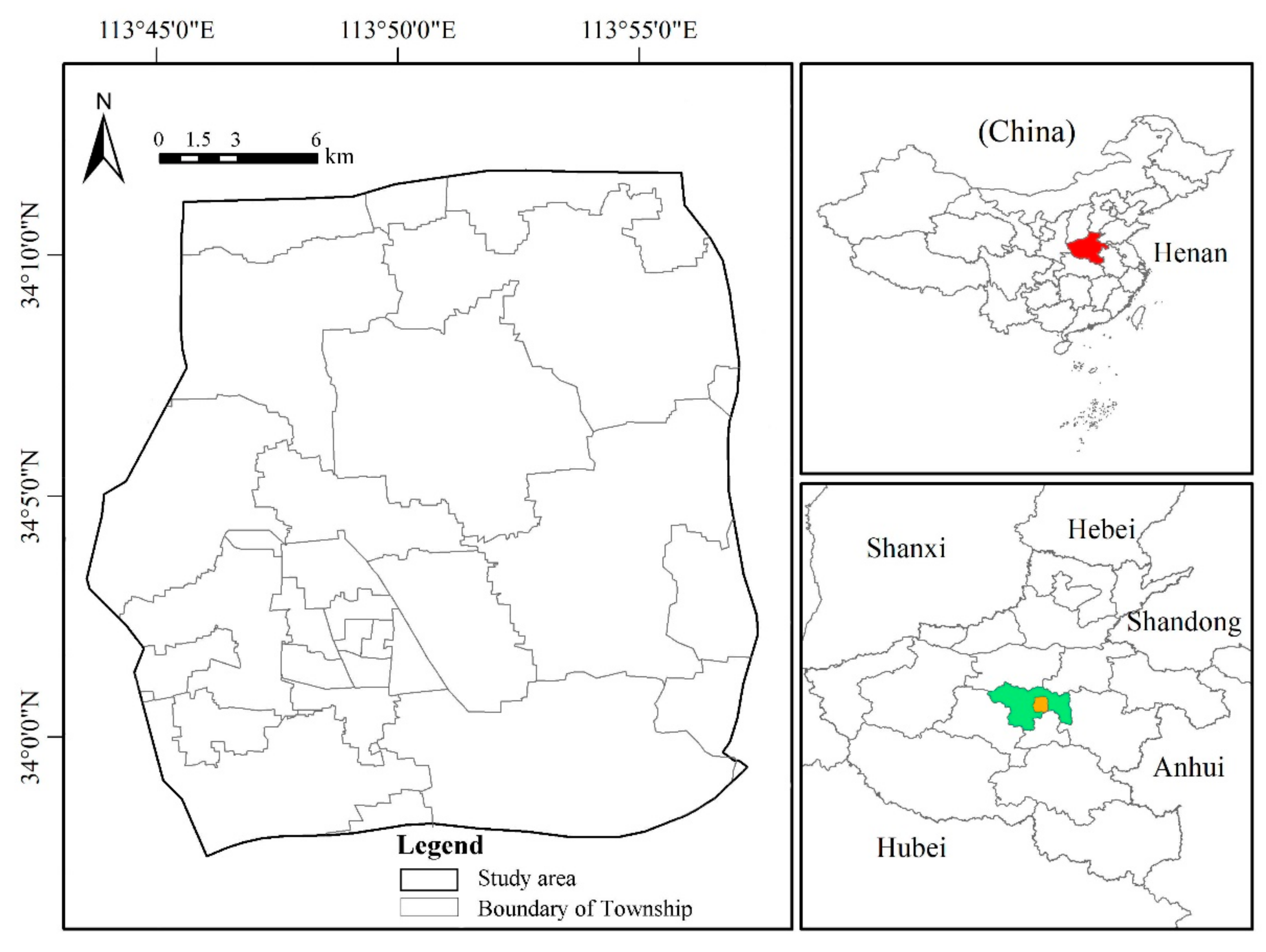
2.1. Study Area

Xuchang City (113°03′–114°19′ E, 33°46′–34°24′ N) is located in the Central Plains of China [44]. It is adjacent to Zhoukou City in the East; Zhengzhou, the capital of the province, to the north; Luohe City in the south; Pingdingshan City in the west; and it is 50 km from Xinzheng International Airport. It is one of the core cities in the Central Plains Urban Agglomeration and Central Plains Economic Zone. With a total area of 4996 km2 and superior natural conditions, the city has a warm temperate continental monsoon climate zone, with an annual average temperature of 14.7 °C. The terrain is high in the northwest and low in the southeast [45]. In addition to other water systems in the city, the three main rivers are Qingshu River, Qingni River, and Yinma River. According to statistics, by the end of 2014, the total population of the city was 4.87 million, and the population of the main urban area was 880,000. In recent years, Xuchang City has made remarkable achievements in green construction and has been awarded successive titles as the “national garden city”, “national forest city”, and “excellent tourism city of China”. As the only national ecological garden city in Central Plains, the green space development and evolution of Xuchang City is typical. According to the construction land balance table for Xuchang City in 2014 and 2030, the increment of green space and square land is 1599.95 ha, accounting for 13.03% in 2030 from 8.96% in 2014. However, the increase of greening quantity does not guarantee that the layout structure is sensible. Therefore, it is necessary to further explore the land conversion to simulate and optimize the green space development layout of the main urban area with high density population. The study area covered 189 km2 (Figure 1) of the main urban area.

2.2. Study Method

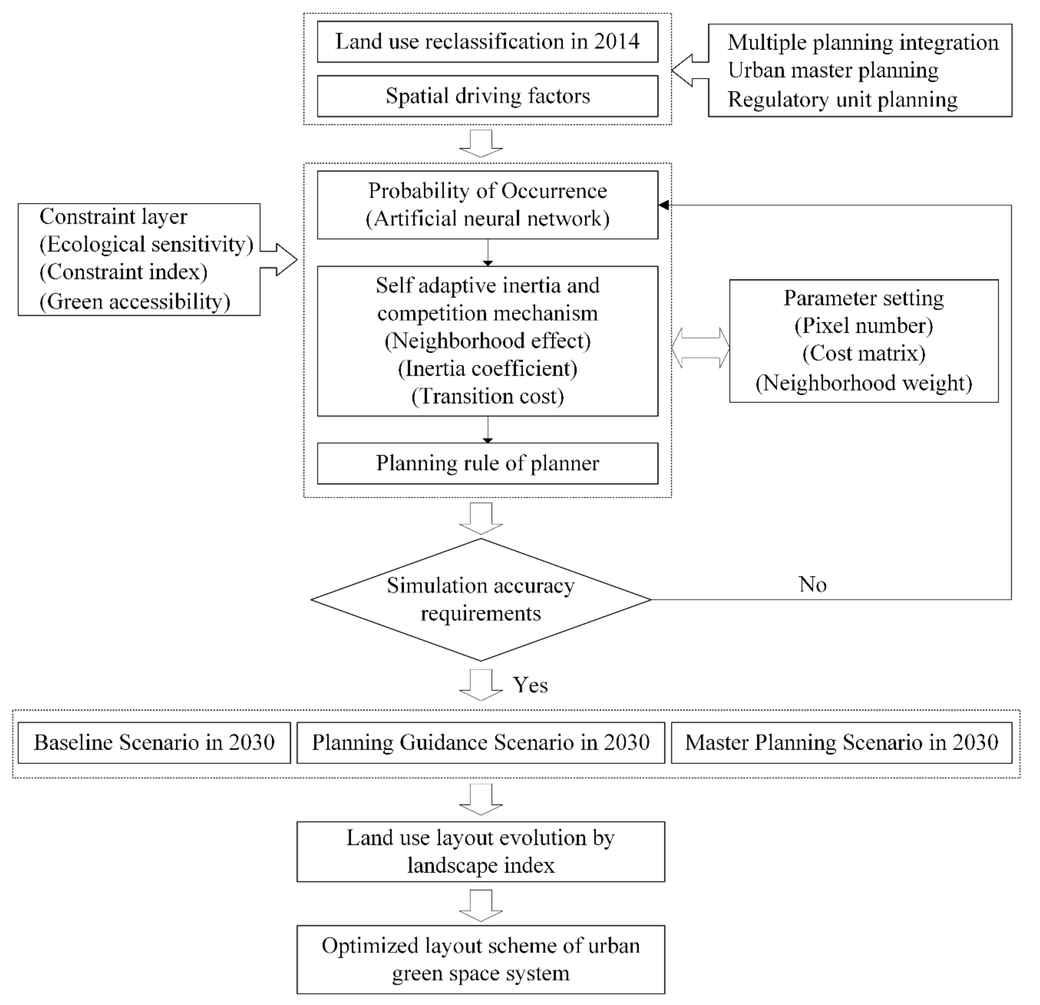
2.2.1. Land Use Layout Simulation

As a critical component of urban construction land, the number and layout of the green space and square land share interrelated temporal and spatial characteristics with other land types [46,47]. In this paper, we combined the evolution of the urban green space system with the development of urban land use. We entered the driving factors and constraints into the FLUS model (www.geosimulation.cn/FLUS.html) to ensure the simulation in a predetermined direction and obtained the layout scheme of the urban green space system.
Based on the CA model, the FLUS model integrates the artificial neural network (ANN) algorithm and the adaptive inertia competition mechanism of roulette. ANN is a type of machine learning model with self-learning, self-organization, and self-adaptiveness; it can effectively solve the nonlinear relationship between land use status data and spatial variables, such as terrain, location, and traffic [48,49,50]. The adaptive inertia competition mechanism based on roulette selection is combined with neighborhood weight (the expansion capacity of land use types driven by external factors), the inertia coefficient (the inheritance of land use types in the iterative process), the conversion cost ( the land use conversion or not), and roulette selection (the opportunity for conversion and distribution of each land use type) to establish a circular iteration between land demand and land status [51,52] in order to make the output value close to the target value.
We used the FLUS model with the ANN algorithm to obtain the development probability of all types of land use in the study scope. The ANN model used in this study included an input layer with six neurons (corresponding to six spatial driving factors), a hidden layer, and an output layer with two neurons (corresponding to urban construction and nonurban construction areas). In essence, the simulation process established the intensity relationship of the interaction between driving factors and land types, and the probability formula can be expressed as follows:
n e t j p , t = i w i j × x i p , t ,
sigmoid n e t j p , t = 1 1 + e n e t j p , t ,   and
p p , k , t = j w j , k × s i g m o i d n e t j p , ,
where n e t j p , t represents the transmission signal received by neuron j, x i p , t is the relationship function between training time t and grid p in input layer neuron i, w i , j is the adaptive weight used for calibration in the training process, and sigmoid n e t j p , t is the correlation function. Different neurons in the output layer represent different land use types; p p , k , t indicates the probability of occurrence (PoO) of land type k in t-time and grid p ; w j , k is similar to w i , j and is the adaptive weight. The neural network model of w j , k and   w i , j after proofreading with training data can be used to calculate the suitability probability of various types of land use.
The neighborhood effect is similar to the traditional CA model. The definition of neighborhood development density of land type k in grid p is as follows:
Ω p , k t = N × N c o n c p t 1 = k N × N 1 × w k ,
where N × N c o n c p t 1 = k represents the total number of grids when the iteration time of land use type k is t 1 in the N × N Moore window. In this study, we selected the 3 × 3 Moore neighborhood model; w k   is the variable weight. The inertia coefficient is based on the current land use situation through the iterative adjustment to the preset demand conversion. The inertia coefficient is defined as:
I n t e r t i a k t =     I n t e r t i a k t 1 i f   D k t 1 D k t 2 I n t e r t i a k t 1 × D k t 2 D k t 1 i f   D k t 1 < D k t 2 < 0 I n t e r t i a k t 1 × D k t 2 D k t 2 i f   0 < D k t 2 < D k t 1
where I n t e r t i a k t represents the inertia coefficient of land use type k   when iteration time is   t , and D k t 1 is the difference between macro demand and land use type k allocation when time is t 1 . The total probability of the unit occupied by a specific land use type can be expressed as follows:
T P p , k t = P p , k × Ω p , k t × I n e r t i a k t × 1 s c c k ,
where T P p , k t indicates the combination probability of grid p from the initial status to the target type k at iteration time t, P p , k   indicates the probability of grid p appearing as the land use type k, Ω p , k t is the neighborhood effect of grid p appearing as the land use type k in iteration, and s c c k indicates the cost of land use type c to k conversion.

2.2.2. Evaluation of the Simulation Scenarios

Each land use type had interrelated temporal and spatial characteristics in the development process. We selected the landscape indexes [53,54,55], which combined information theory and fractal geometry, to analyze the land use of green space and square land. The landscape indexes were divided into three levels: patch, type, and landscape [56]. At the type level, we selected the Edge Density (ED) in the edge index system to measure the complexity of the boundary and the fragmentation degree of the landscape type. The Mean Fractal Dimension Index (FRAC_MN) in the shape index system was used to measure the morphological complexity and compactness of the landscape; the Mean Euclidean Nearest Neighbor Distance (ENN_MN) in the proximity index system was used to measure the size of the research space and the relationship between the land patches. Three landscape indexes were calculated by FRAGSTATS [57]. The specific simulation chart is shown in Figure 2.

2.3. Data Basis and Preprocessing

Data preparation consisted of three parts: a land use data layer, a driving factor data layer, and a restriction and guidance data layer. We preprocessed data to rasterize all of the data. In the process of rasterization, we resampled all of the layers at a spatial resolution of 10 m × 10 m. In addition, we clipped all of the layers by the same research area boundary to ensure that the number of rows and columns of all of the images were the same.

2.3.1. Data Sources

The 2014 land use map of the main urban area of Xuchang City and the urban land use planning map of 2030 were used for basic data. We regarded the Current land use classification (GB/T 21010-2017) [58], Code for classification of urban land use and planning standards of development land (GB50137-2011) [59], Standard for classification of urban green space (CJJ/T85-2017) [60], Technical code for delineation of urban green line (GB/T51163-2016) [61], Xuchang City Master Plan (2015–2030) (www.xuchang.gov.cn/), Xuchang City Green Space System Plan (2015–2030) (www.xuchang.gov.cn/), and other documents as important references. Considering the operability of the study and the elastic adjustment of the unit control rules for the property of the plot [62,63], the land use type and the green land rate index of the construction land types were used as the basis for the classification of the types of land use. We extracted the following seven categories (Table 1): (1) green space and square land, (2) residential land, (3) industrial land, (4) commercial services land, (5) water area, (6) agricultural and forestry land, and (7) village and town construction land.

2.3.2. Parameter Settings

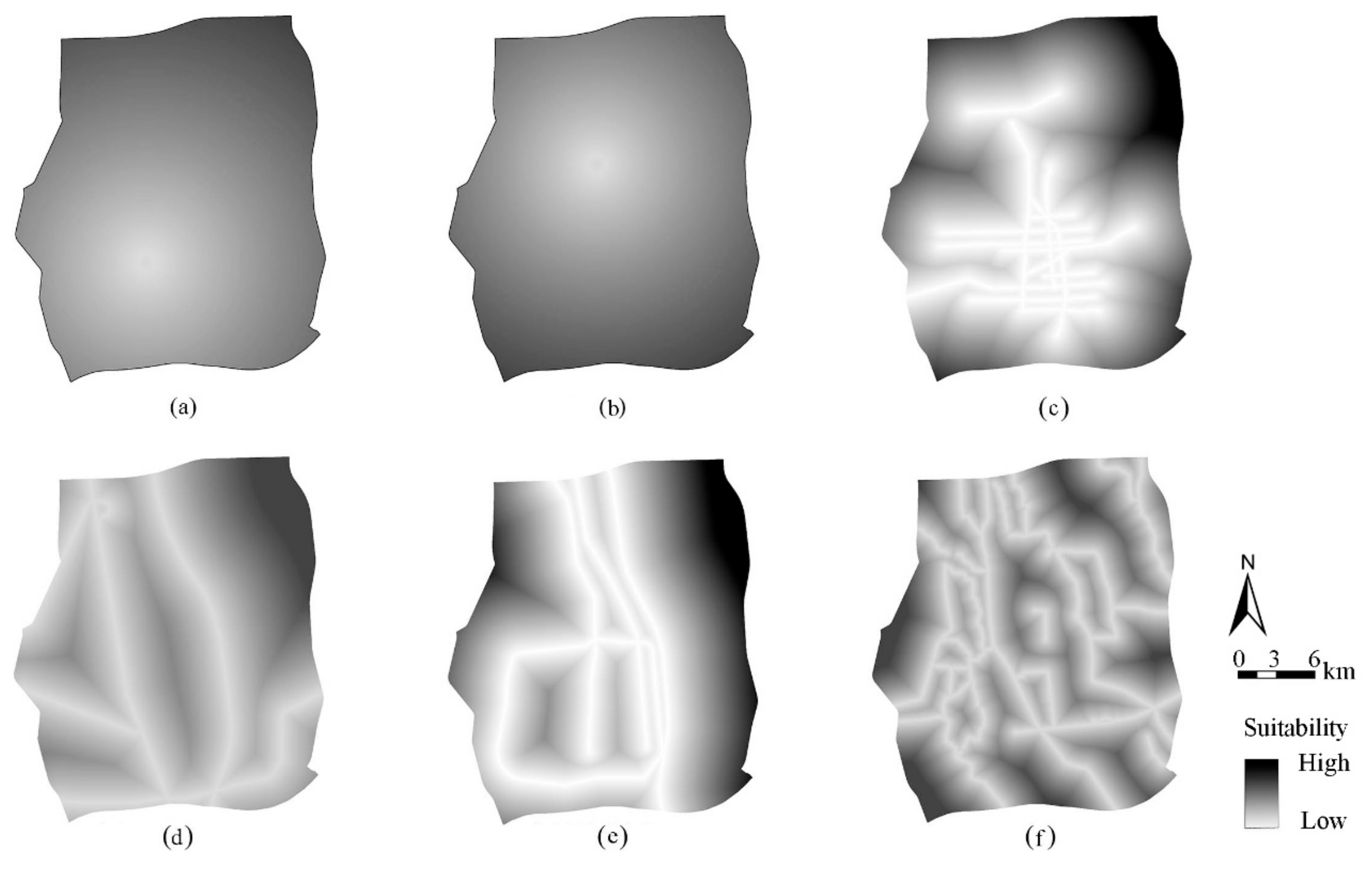
Parameter Identification of Spatial Driving Factors

Spatial factors are independent variables, which were selected by considering the inheritance of land use conversion and the suitability of regional development [64]. We conducted uniform sampling in the study area, excavated six inertia-influencing factors that affected spatial development according to a logistics regression model, and identified the parameters. The constant term was −1.621. The parameter values of spatial factors, as shown in Figure 3 and Table 2, reflect the degree of influences of spatial factors on land use development. If the value was negative, the greater the absolute value was, the stronger the guiding effect of this factor was on land development.

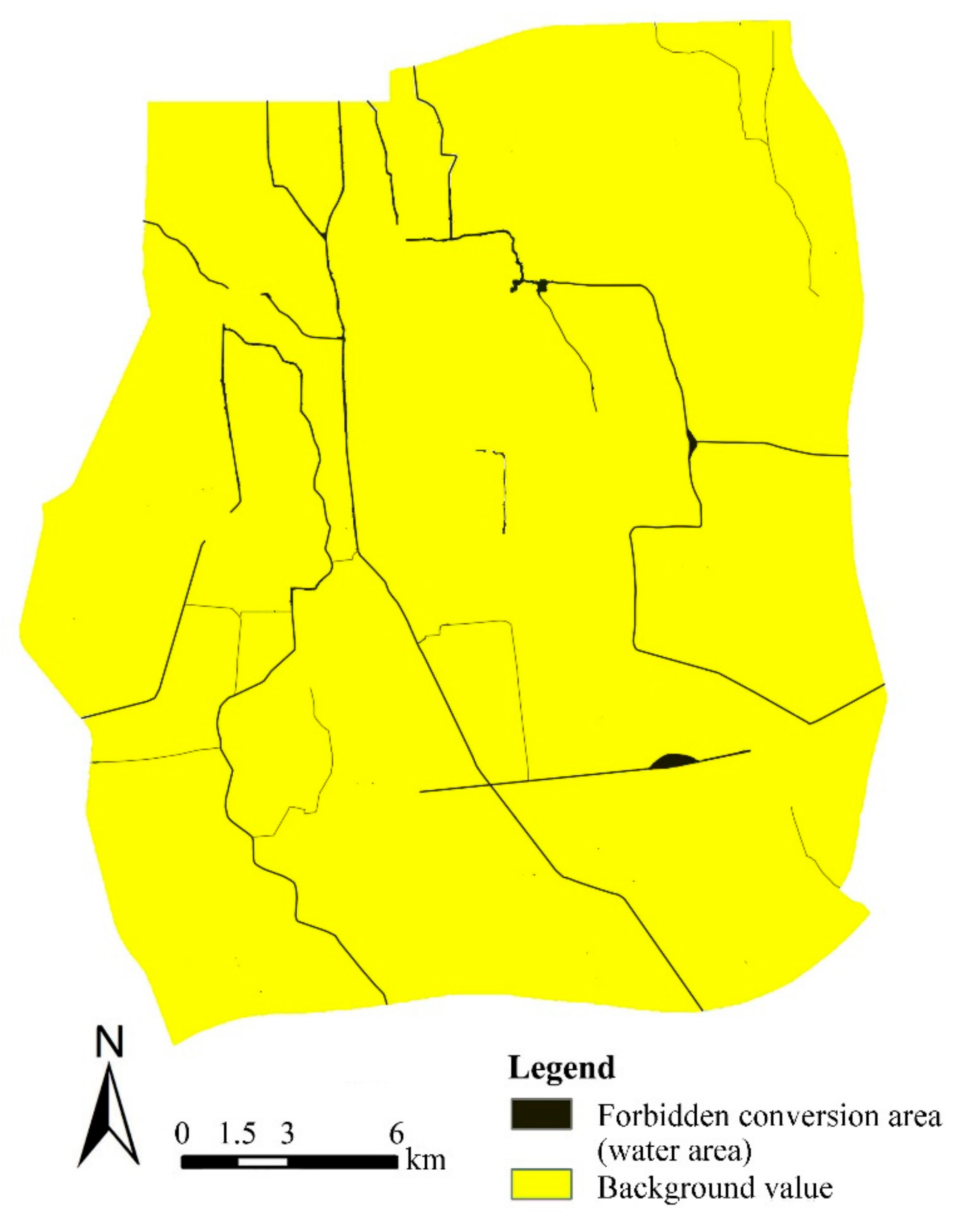
Restrictions on Space Development

From the perspective of ecological sensitivity analysis and ecological space protection, we set the forbidden conversion area in the FLUS model. According to the “Special planning of Xuchang City ecological restoration (2018–2035)” (www.xuchang.gov.cn/), the high-sensitivity area accounted for 10%, the medium-sensitivity area accounted for 10%, the low-sensitivity area accounted for 29%, and the non-sensitivity area accounted for 51%. We selected the water area as the ecologically sensitive zone, and the land use type was prohibited from being converted in the FLUS model (Figure 4).

Relevant Planning Polices and Index Constraints

In this study, we integrated a spatial development strategy and planning index system by coordinating “green space planning” with “urban planning” and “land use planning.” According to the abovementioned plannings in Xuchang City, the spatial expansion direction of the main urban area was a “northward, group growth, banded link”, and the spatial expansion mode was described as follows: “the main mode is axial band expansion, and the secondary mode is compact circle expansion” (Figure 5a). The green space system was planned as a multilevel integrated structure of both agglomeration and division (Figure 5b), including points (garden square), lines (ecological corridor, protective green belt, and riverside landscape belt), and areas (park green space, ecological wetland, and peripheral ecological leisure area). Considering the service radius coverage requirements for parks of National Ecological Garden City, the layout was guided by “300 meters green, 500 meters garden”. The influence of the external space development of the main urban area and the improvement of the layout of the internal green space system were transformed into parameters by the gravity field model [65,66] (Figure 5c).
In the current built-up area of Xuchang City, the ratio of green space is 34.73%, the ratio of greenery coverage is 39.84%, and the per capita park green area is 9.85 m2. By 2030, the ratio of green space of the built-up area in the Xuchang main urban area will be ≥ 44.8%, the ratio of greenery coverage will be ≥ 50.2%, and the per capita park green area will be ≥ 16.2 m2. The balance of urban and rural land use in the main urban area of Xuchang City is shown in Table 3. The data reflect the variation of rural residential land, water area, and agricultural and forestry land. The balance of urban construction land is shown in Table 4, which reflects the changing trend of the four reclassified land uses. The attached urban green space is a vital part of the planned space and does not balance urban construction land on its own. Because of its complexity, previous studies often have ignored the role of attached green space in urban space. In our model, each land type change value and green space index constraint (Table 5) were considered as the pivotal influencing factors, which affected the parameter setting of the cost matrix and the neighborhood weight. Among these factors, the area change reflected the development and expansion ability of the land, and the green space ratio of each land type reflected the difficulty and the possibility of land conversion.

Model Parameter Settings

In the FLUS model, the number of iterations, size of the neighborhood range, acceleration factor of the model and quantity target, cost matrix, and neighborhood factor all needed to be tested. We set the initial iteration number as 300, the Moore neighborhood as 3 × 3, and the acceleration factor as 0.1. We determined the input of the target pixel quantity according to the quantity demand for each type of land use in the master plan (Table 6). To determine the cost matrix and neighborhood factors, we considered variations in each land type, land cost, and green land ratio, and assigned values according to the difficulty and expansion ability of each land type [67]. In addition, in the process of urban land expansion, green space and square land, ecological space generally cannot be occupied. Considering the land cost and the conversion threshold between each land type—that is, commercial services land > residential land > industrial land—we did not convert residential land and commercial services into industrial land. The specific restriction matrix is shown in Table 7. If conversion was allowed among different types of land, the parameter was 1, and if it was not allowed, the parameter was 0. For neighborhood weight, we took the scale variables of the base period and target year of each land use type as the reference to set conversion intensity parameters. The specific settings are given in Table 8.

3. Results and Analysis

3.1. Scenario Simulation of Land Use Layout

Based on the status 2014, this study simulated different urban land use layout scenarios under natural effects and human interventions. We developed three scenarios according to different spatial planning policies and constraint conditions: (1) the 2030 Baseline Scenario, (2) the 2030 Planning Guidance Scenario, and (3) the 2030 Master Plan Scenario. In the first scenario, there were no constraint variables such as ecological space protection and residents’ demands for green space. The developed land use model was based on natural spatial driving factors. However, in order to avoid the generation of urban land use scenario with unconstrained form, the quantitative index in planning was used as the reference to set the transformation parameters among each land type. The suitability probability map (Figure 6) was obtained by training the ANN model; the higher the value was, the greater the probability of each land use type occurred. The map had seven bands, each of which corresponded to the PoO of one land use type. Additionally, we transformed the quantitative constraint indexes of relevant planning (mentioned in Section 2.3.2) into a combined parameter of the adaptive inertia competition mechanism. Based on the Status Scenario in 2014 (Figure 7a), the 2030 Baseline Scenario (Figure 7b) was generated by introducing planning rules developed by planner agents [5,68].
In order to prevent the occupation from the construction land to the ecological space, the ecological space protection was considered as a variable in constraint layer. Besides, the relationship between the accessibility of urban green space and residents’ well-being was taken into consideration. Taking the residents’ demand for green space as a variable, the possibility and potential of providing services to residents of urban park green space were measured so as to optimize the layout of urban green space. Therefore, we designed the second scenario. We embedded the constraint layers into the FLUS model through the gravity field model and generated the urban land use layout scheme in the 2030 Planning Guidance Scenario (Figure 7c). This scenario coordinated the transformation relationship of urban and rural land in the main urban area and coordinated the relationship of urban green space and other land types in construction land. In addition, according to Xuchang City Master Plan (2015–2030) (www.xuchang.gov.cn/), the 2030 Master Plan Scenario is shown as Figure 7d.

3.2. Analysis of Simulation Results

We used the root mean square error (RMSE) of the probability of suitability occurrence module and the Kappa coefficient of the overall model simulation accuracy verification index to evaluate the feasibility of the FLUS model. The mode of ANN training samples includes uniform sampling and random sampling; uniform sampling (10/1000) was used in this study. The Kappa coefficients of the Baseline Scenario and the Planning Guidance Scenario were 0.5814 and 0.6036, respectively. The RMSE of this operation was 0.2589. The simulation accuracy of the model was within the precision range. Compared with the Master Plan Scenario in 2030, the simulation results were complied with the objective rules of current urban development.
The calculation results of spatial index are shown in Table 9. We combined these results with the multi-scenario simulation and planning scheme. The characters of the Baseline Scenario could be described as urban land use development that was coordinated with the spatial factors. New land development was more likely to occur near the current traffic network. The spatial expansion of the city showed a trend that looked like a “spreading pancake”, which depended significantly on the distribution of the urban traffic network. Residential land expanded to the southwest, whereas industrial land expanded to the northeast. Commercial land tended to be distributed toward the margins, and the green space and square land showed a disordered development trend. Overall, the distribution of urban land was relatively scattered, which did not meet the development needs of Xuchang City in the planning period and did not consider urban residents’ demand for urban parks and green space. Under the Master Plan Scenario, urban space represented an ideal expansion trend. Compared with the Baseline Scenario, urban construction land as a whole was characterized by a more compact evolution, and green space and square land was characterized by a networked and customized layout. These trends guaranteed the basic quantitative index requirements of urban space development and green space system evolution; however, because of other spatial restrictions, the actual urban land development will not evolve completely in accordance with the planning. In addition, this scenario lacks the consideration of the service capacity of urban green space. Under the Planning Guidance Scenario, we combined the expansion strategy of urban space with the development process of urban space. The expansion mode was mainly northward and axially banded, which made the evolution simulation result more intensive and efficient. To meet the coverage rate of 90% of the service radius for parks in Xuchang City, we guided the layout evolution of green space and square land to improve the service function of the urban green space system.

4. Discussion

In previous studies, urban construction land usually has been regarded as a land type with which to explore the expansion process and its impact on natural resources [69]. The innovation in this study was that the evolution process of all kinds of land types within the main urban area of a city was considered and the constraint conditions were embedded into the FLUS model. These constraints included an urban development strategy [70,71], the accessibility of the green space of the park [72], and the sensitivity of the ecological space [73]. Additionally, while considering different goals, this study discussed the possibility of the development and evolution of an urban space and urban green space system, which mainly served the needs of urban residents.
The function of ecosystem service is affected by the dynamic change of landscape pattern [74]. Improving the service function of an ecosystem is not only the goal of urban planning but also an important basis by which urban planning is evaluated. The layout of urban land has an impact on the ecological processes such as material exchange, soil and water conservation, and biological cycle [75]. Through the adjustment of the land conversion process, the transformation of ecosystem service type can be realized. In this study, we used the landscape index to evaluate the simulation results. However, the existing landscape indexes were redundant [76]. On the basis of fully understanding the previous studies as well as the ecological significance of landscape indexes, we selected the ED, FRAC_MN, and ENN_MN from the type levels, which objectively reflected the rationality of the land use patterns.
Urban planning is a continuous process. The unit control plan guided by the “dynamic balance control of unit total amount” is an effective layer, which links the two levels, that is, master planning and detailed planning. This plan can be used to effectively allocate urban land resources and promote multilevel effective control of land and space. On the basis of the “multiple planning integration” of spatial planning and the elastic adjustment of the plot nature, this study reclassified urban land and compared the land simulation results with the existing planning. This simulation provided a means to actively explore and promote the technical transformation of the planning work from “static results” to a “dynamic process”.
Future research will focus on the following:
(1)
Model parameters setting. In addition to spatial location influencing factors, driving factors, such as economy and population, could be added as well as time variation and spatial differentiation of planning policies and constraint indicators [77]. While considering the protection of ecological space and the accessibility of green spaces, the connectivity of green space also could be taken as an important variable to optimize the layout from the perspective of biodiversity [78,79,80]. In addition, this study also tested the parameter combination of self-adaptive inertia and the competition mechanism of the CA module to obtain an optimal combination. It should combine planning rules to improve the accuracy of the simulation results.
(2)
Research object level. According to the latest Standard for classification of urban green space (CJJ/T85-2017) [60], this research can be extended to examine the relationship between regional green space and urban construction land development, as well as the external correlation and agglomeration effect of various green space types within urban construction land. In addition, the layout optimization, as well as intensive and efficient development of urban land should be discussed at multiple levels and scales [81,82].
(3)
Planning rigidity and flexibility. The requirements of land use properties and development intensity of various types of urban land are dynamic. The control indicators based on the land plot are too rigid to respond in a timely fashion to the future development scenario of the city. Thus, the planning of “blank” and elastic spaces should be considered to better connect the planning system [83,84].

5. Conclusions

We presented a new method to simulate the evolution of urban green space system in the main urban area of Xuchang City based on the FLUS model. In this approach, we calculated the probability of the occurrence of future land use according to ANN. We simulated the spatial layout of land use in 2030 using an adaptive inertia competition mechanism and planning rules. The Baseline Scenario and Planning Guidance Scenario were generated. Then, we used landscape indices to evaluate these scenarios combined with the Master Plan Scenario. We reached the following main conclusions.
The RMSE of probability of the suitability occurrence module and the Kappa coefficients of the Baseline Scenario and the Planning Guidance Scenario were all within the range of accuracy requirements. The results show that the FLUS model, which embeds the variables, including ecological space protection, accessibility of park green space, and planning quantitative index, can realize the simulation of urban land use development in medium- and long-term planning.
Under the Baseline Scenario, the spatial expansion was similar to that of a “spreading pancake” without spatial constraints contributed to the scattered layout of the urban land and the disordered development of urban green space. Compared with the Baseline Scenario, the Master Plan Scenario had a more compact urban land use layout, and the green space system was characterized by networking and systematization, but the service capacity of green space was not considered. The Planning Guidance Scenario considered the introduction of constraint conditions had more intensive and efficient use of urban spaces and provided a better functioning green space system layout. Through the multi-scenario simulation, we concluded that urban development schemes under the natural spatial driving factors and the existing planning were not the recommended model for the efficient development of urban land. The urban development scheme, which considered ecology (ecological space protection), production (urban-rural relationship coordination), and life (residents’ demand for the urban green space), had better structural and functional characteristics. This is in accordance with the current emphasis on “ecological-production-living space” in the optimization of China’s national territory spatial pattern [85,86].
The research results enable managers and planners to evaluate the development mode of the urban green space system coupled with land use evolution and to adjust the implementation process of urban planning so as to promote efficiency, scientific nature, and flexibility.

Author Contributions

Conceptualization, J.L. and L.Z.; Methodology, J.L.; Software, J.L.; Validation, J.L., Q.Z., and L.Z.; Formal analysis, J.L.; Investigation, J.L. and L.Z.; Resources, L.Z.; Data curation, J.L., L.Z., and Q.Z.; Writing—original draft preparation, J.L.; Writing—review and editing, L.Z. and Q.Z.; Visualization, J.L.; Supervision, L.Z. and Q.Z.; Project administration, J.L. and Q.Z.; Funding acquisition, J.L., L.Z., and Q.Z. All authors have read and agreed to the published version of the manuscript.

Funding

This research was funded by the National Key R&D Program of China (2017YFC0505706) and the Postgraduate Research & Practice Innovation Program of Jiangsu Province (KYCX18_0978).

Acknowledgments

The authors would like to thank our editors, the anonymous reviewers for their valuable comments, and also LetPub (www.letpub.com) for linguistic assistance during the preparation of this manuscript.

Conflicts of Interest

The authors declare no conflict of interest.

References

  1. Lu, Y.; Wang, R.; Zhang, Y.; Su, H.; Wang, P.; Jenkins, A.; Ferrier, R.C.; Bailey, M.; Squire, G. Ecosystem health towards sustainability. Ecosyst. Heal. Sustain. 2015, 1, 1–15. [Google Scholar] [CrossRef]
  2. Southon, G.E.; Jorgensen, A.; Dunnett, N.; Hoyle, H.; Evans, K.L. Perceived species-richness in urban green spaces: Cues, accuracy and well-being impacts. Landsc. Urban Plan. 2018, 172, 1–10. [Google Scholar] [CrossRef]
  3. Wang, Y.C.; Shen, J.K.; Xiang, W.N. Ecosystem service of green infrastructure for adaptation to urban growth: Function and configuration. Ecosyst. Heal. Sustain. 2018, 4, 132–143. [Google Scholar] [CrossRef]
  4. Verdú-Vázquez, A.; Fernández-Pablos, E.; Lozano-Diez, R.V.; López-Zaldívar, Ó. Development of a methodology for the characterization of urban and periurban green spaces in the context of supra-municipal sustainability strategies. Land Use Policy 2017, 69, 75–84. [Google Scholar] [CrossRef]
  5. Long, Y.; Gu, Y.; Han, H. Spatiotemporal heterogeneity of urban planning implementation effectiveness: Evidence from five urban master plans of Beijing. Landsc. Urban Plan. 2012, 108, 103–111. [Google Scholar] [CrossRef]
  6. Haaland, C.; van den Bosch, C.K. Challenges and strategies for urban green-space planning in cities undergoing densification: A review. Urban For. Urban Green. 2015, 14, 760–771. [Google Scholar] [CrossRef]
  7. Baycan-Levent, T.; Nijjkamp, P. Planning and management of urban green spaces in Europe: Comparative analysis. J. Urban Plan. Dev. 2009, 135, 1–12. [Google Scholar] [CrossRef]
  8. Tiba, C.; Candeias, A.L.B.; Fraidenraich, N.; Barbosa, E.M.d.S.; de Carvalho Neto, P.B.; de Melo Filho, J.B. A GIS-based decision support tool for renewable energy management and planning in semi-arid rural environments of northeast of Brazil. Renew. Energy 2010, 35, 2921–2932. [Google Scholar] [CrossRef]
  9. Hopkins, L. Book Review: Planning support systems for cities and regions. Int. J. Geogr. Inf. Sci. 2011, 25, 324–325. [Google Scholar] [CrossRef]
  10. Cerreta, M.; De Toro, P. Urbanization suitability maps: A dynamic spatial decision support system for sustainable land use. Earth Syst. Dyn. 2012, 3, 157–171. [Google Scholar] [CrossRef] [Green Version]
  11. Jin, Y.; Liu, S.; Li, R.; Liu, Y. Urban Green Space System Planning Formulation—Research on “Subsystem” Planning Method. Chin. Landsc. Archit. 2013, 29, 56–59. [Google Scholar]
  12. Xu, C.; Haase, D.; Pribadi, D.O.; Pauleit, S. Spatial variation of green space equity and its relation with urban dynamics: A case study in the region of Munich. Ecol. Indic. 2018, 93, 512–523. [Google Scholar] [CrossRef]
  13. Zhang, Y.; Feng, G. Study on dynamic land use planning. China Land. Sci. 2017, 31, 25–32. [Google Scholar]
  14. Batty, M. The size, scale, and shape of cities. Science. 2008, 319, 769–771. [Google Scholar] [CrossRef] [Green Version]
  15. Spencer, D. Cities and Complexity: Understanding Cities with Cellular Automata, Agent-Based Models, and Fractals. J. Archit. 2009, 14, 446–450. [Google Scholar] [CrossRef]
  16. Xiang, W.N.; Clarke, K.C. The use of scenarios in land-use planning. Environ. Plan. B Plan. Des. 2003, 30, 885–909. [Google Scholar] [CrossRef] [Green Version]
  17. Sohl, T.L.; Sleeter, B.M.; Sayler, K.L.; Bouchard, M.A.; Reker, R.R.; Bennett, S.L.; Sleeter, R.R.; Kanengieter, R.L.; Zhu, Z. Spatially explicit land-use and land-cover scenarios for the Great Plains of the United States. Agric. Ecosyst. Environ. 2012, 153, 1–15. [Google Scholar] [CrossRef] [Green Version]
  18. Liu, J.; Zhang, L.; Ji, Y.; Zhang, Q. Spatial-temporal Evolution Analysis of Urban Green Space System Based on Fractal Model: A Case Study of Downtown Shanghai. Mod. Urban Res. 2019, 12–19. [Google Scholar]
  19. Liu, Y.; Wang, J. Theoretical analysis and technical methods of “multiple planning integration” in the rural to urban transition period in China. Prog. Geogr. 2016, 35, 529–536. [Google Scholar]
  20. Liu, Y.; Fang, F.; Li, Y. Key issues of land use in China and implications for policy making. Land Use Policy 2014, 40, 6–12. [Google Scholar] [CrossRef]
  21. Batty, M.; Xie, Y. From cells to cities. Environ. Plan. B Plan. Des. 1994, 21, 531–548. [Google Scholar] [CrossRef]
  22. Yeh, A.G.O.; Li, X. Errors and uncertainties in urban cellular automata. Comput. Environ. Urban Syst. 2006, 30, 10–28. [Google Scholar] [CrossRef]
  23. Hamad, R.; Balzter, H.; Kolo, K. Predicting land use/land cover changes using a CA-Markov model under two different scenarios. Sustainable 2018, 10, 3421. [Google Scholar] [CrossRef] [Green Version]
  24. Li, X.; Yeh, A.G. Modelling sustainable urban development by the integration of constrained cellular automata and GIS. Int. J. Geogr. Inf. Sci. 2010, 14, 37–41. [Google Scholar] [CrossRef]
  25. Wickramasuriya, R.C.; Bregt, A.K.; van Delden, H.; Hagen-Zanker, A. The dynamics of shifting cultivation captured in an extended Constrained Cellular Automata land use model. Ecol. Modell. 2009, 220, 2302–2309. [Google Scholar] [CrossRef]
  26. White, R.; Engelen, G.; Uljee, I. The use of constrained cellular automata for high-resolution modelling of urban land-use dynamics. Environ. Plan. B Plan. Des. 1997, 24, 323–343. [Google Scholar] [CrossRef]
  27. Li, X.; Ye, J. Constrained Cellular Automata for modelling sustainable urban Forms. Acta Geogr. Sin. 1999, 54, 289–298. [Google Scholar]
  28. Zhang, Y.; Li, X.; Liu, X.; Qiao, J. Self-modifying CA model using dual ensemble Kalman filter for simulating urban land-use changes. Int. J. Geogr. Inf. Sci. 2015, 29, 1612–1631. [Google Scholar] [CrossRef]
  29. Liu, X.; Liang, X.; Li, X.; Xu, X.; Ou, J.; Chen, Y.; Li, S.; Wang, S.; Pei, F. A future land use simulation model (FLUS) for simulating multiple land use scenarios by coupling human and natural effects. Landsc. Urban Plan. 2017, 168, 94–116. [Google Scholar] [CrossRef]
  30. Liang, X.; Liu, X.; Li, X.; Chen, Y.; Tian, H.; Yao, Y. Delineating multi-scenario urban growth boundaries with a CA-based FLUS model and morphological method. Landsc. Urban Plan. 2018, 177, 47–63. [Google Scholar] [CrossRef]
  31. Chen, Y.; Li, X.; Liu, X.; Ai, B.; Li, S. Capturing the varying effects of driving forces over time for the simulation of urban growth by using survival analysis and cellular automata. Landsc. Urban Plan. 2016, 152, 59–71. [Google Scholar] [CrossRef]
  32. Wu, F. A linguistic cellular automata simulation approach for sustainable land development in a fast growing region. Comput. Environ. Urban Syst. 1996, 20, 367–387. [Google Scholar] [CrossRef]
  33. Itami, R.M. Simulating spatial dynamics: Cellular automata theory. Landsc. Urban Plan. 1994, 30, 27–47. [Google Scholar] [CrossRef]
  34. Zhou, C.; Sun, Z.; Xie, Y. Geographical Cellular Automata; Science Press: Beijing, China, 1999. [Google Scholar]
  35. Islam, K.; Rahman, M.F.; Jashimuddin, M. Modeling land use change using Cellular Automata and Artificial Neural Network: The case of Chunati Wildlife Sanctuary, Bangladesh. Ecol. Indic. 2018, 88, 439–453. [Google Scholar] [CrossRef]
  36. Huang, D.; Huang, J.; Liu, T. Delimiting urban growth boundaries using the CLUE-S model with village administrative boundaries. Land Use Policy 2019, 82, 422–435. [Google Scholar] [CrossRef]
  37. Li, X.; Li, D.; Liu, X.; He, J. Geographical Simulation and Optimization System(GeoSOS) and Its Cutting-edge Researches. Adv. Earth Sci. 2009, 24, 899–907. [Google Scholar]
  38. Liang, X.; Liu, X.; Li, D.; Zhao, H.; Chen, G. Urban growth simulation by incorporating planning policies into a CA-based future land-use simulation model. Int. J. Geogr. Inf. Sci. 2018, 32, 2294–2316. [Google Scholar] [CrossRef]
  39. Lu, L.; Weng, Q.; Guo, H.; Feng, S.; Li, Q. Assessment of urban environmental change using multi-source remote sensing time series (2000–2016): A comparative analysis in selected megacities in Eurasia. Sci. Total Environ. 2019, 684, 567–577. [Google Scholar] [CrossRef]
  40. Stone, B.; Hess, J.J.; Frumkin, H. Urban form and extreme heat events: Are sprawling cities more vulnerable to climate change than compact cities? Environ. Health Perspect. 2010, 118, 1425–1428. [Google Scholar] [CrossRef] [Green Version]
  41. Howard, E. Garden Cities of To-morrow; MIT Press: Massachusetts, MA, USA, 1965. [Google Scholar]
  42. Lindley, S.; Pauleit, S.; Yeshitela, K.; Cilliers, S.; Shackleton, C. Rethinking urban green infrastructure and ecosystem services from the perspective of sub-Saharan African cities. Landsc. Urban Plan. 2018, 180, 328–338. [Google Scholar] [CrossRef] [Green Version]
  43. Ramyar, R.; Saeedi, S.; Bryant, M.; Davatgar, A.; Mortaz Hedjri, G. Ecosystem services mapping for green infrastructure planning–The case of Tehran. Sci. Total Environ. 2019, 135466, (Online). [Google Scholar] [CrossRef]
  44. Qu, C.; Meng, Q. Study on functional zoning of land use in Xuchang City. China L. Sci. 2008, 22, 51–55. [Google Scholar]
  45. Wu, G.; Yin, X.; Shen, H. Study on land use/land cover changes in Xuchang City based on GIS. Res. Soil Water Conserv. 2009, 16, 131–134. [Google Scholar]
  46. Belmeziti, A.; Cherqui, F.; Kaufmann, B. Improving the multi-functionality of urban green spaces: Relations between components of green spaces and urban services. Sustain. Cities Soc. 2018, 43, 1–10. [Google Scholar] [CrossRef]
  47. Lynch, A.J. Is it good to be green? Assessing the ecological results of county green infrastructure planning. J. Plan. Educ. Res. 2016, 36, 90–104. [Google Scholar] [CrossRef]
  48. Li, X.; Yeh, A.G.O. Neural-network-based cellular automata for simulating multiple land use changes using GIS. Int. J. Geogr. Inf. Sci. 2002, 16, 323–343. [Google Scholar] [CrossRef]
  49. Almeida, C.M.; Gleriani, J.M.; Castejon, E.F.; Soares-Filho, B.S. Using neural networks and cellular automata for modelling intra-urban land-use dynamics. Int. J. Geogr. Inf. Sci. 2008, 22, 943–963. [Google Scholar] [CrossRef]
  50. Openshaw, S. Neural network, genetic, and fuzzy logic models of spatial interaction. Environ. Plan. A 1998, 30, 1857–1872. [Google Scholar] [CrossRef]
  51. Aerts, J.C.J.H.; Heuvelink, G.B.M. Using simulated annealing for resource allocation. Int. J. Geogr. Inf. Sci. 2002, 16, 571–587. [Google Scholar] [CrossRef] [Green Version]
  52. Huang, K.; Liu, X.; Li, X.; Liang, J.; He, S. An improved artificial immune system for seeking the Pareto front of land-use allocation problem in large areas. Int. J. Geogr. Inf. Sci. 2013, 27, 922–946. [Google Scholar] [CrossRef]
  53. McGarigal, K.; Marks, B.J. FRAGSTATS: Spatial Patten Anaylsis Program for Quantifyling Landscape Structure; US Forest Service Pacific Northwest Research Station: Portland, Oregon, 1994.
  54. Yang, X.; Zheng, X.Q.; Chen, R. A land use change model: Integrating landscape pattern indexes and Markov-CA. Ecol. Modell. 2014, 283, 1–7. [Google Scholar] [CrossRef]
  55. Xing, H.; Meng, Y. Measuring urban landscapes for urban function classification using spatial metricsing spatial metrics. Ecol. Indic. 2020, 108. [Google Scholar] [CrossRef]
  56. Wu, J. Landscape Ecology: Pattern, Process, Scale and Hierarchy; Higher Education Press: Beijing, China, 1974. [Google Scholar]
  57. Tian, G.; Ouyang, Y.; Quan, Q.; Wu, J. Simulating spatiotemporal dynamics of urbanization with multi-agent systems-A case study of the Phoenix metropolitan region, USA. Ecol. Modell. 2011, 222, 1129–1138. [Google Scholar] [CrossRef]
  58. AQSIQ. Current Land Use Classification; General Administration of Quality Supervision, Inspection and Quarantine of the People’s Republic of China/Standardization Administration: Beijing, China, 2017. [Google Scholar]
  59. MOHURD. Code for Classification of Urban Land Use and Planning Standards of Development Land; Ministry of Housing and Urban-Rural Development of the People’s Republic of China (MOHURD): Beijing, China, 2011.
  60. MOHURD. Standard for Classification of Urban Green Space; Ministry of Housing and Urban-Rural Development of the People’s Republic of China (MOHURD): Beijing, China, 2017.
  61. MOHURD. Technical Code for Delineation of Urban Green Line; Ministry of Housing and Urban- Rural Development of the People’s Republic of China (MOHURD): Beijing, China, 2016.
  62. Chen, S.; Yang, Z.; Wang, Z. “Grey Land” planning: A flexible control method to coordinate short-term and long-term land use of atrophic urban fringe. Urban Dev. Stud. 2016, 2016, 70–77. [Google Scholar]
  63. Yang, Z.; Wang, Z. Research on flexible control method of land use in new town planning: A case study of Hangzhou Bay New Town. City Plan. Rev. 2014, 38, 43–49, 58. [Google Scholar]
  64. Santé, I.; García, A.M.; Miranda, D.; Crecente, R. Cellular automata models for the simulation of real-world urban processes: A review and analysis. Landsc. Urban Plan. 2010, 96, 108–122. [Google Scholar] [CrossRef]
  65. Zhou, T.; Guo, D. GIS-based researches on urban green space on landscape gravity field with Ningbo city as an example. Acta Ecol. Sin. 2004, 24, 1157–1163. [Google Scholar]
  66. Siewwuttanagul, S.; Inohae, T.; Mishima, N. An investigation of Urban Gravity to develop a better understanding of the urbanization phenomenon using centrality analysis on GIS platform. Procedia Environ. Sci. 2016, 36, 191–198. [Google Scholar] [CrossRef] [Green Version]
  67. Dahal, K.R.; Chow, T.E. Characterization of neighborhood sensitivity of an irregular cellular automata model of urban growth. Int. J. Geogr. Inf. Sci. 2015, 29, 475–497. [Google Scholar] [CrossRef]
  68. Brail, R.K. Planning Support Systems for Cities and Regions; Lincoln Institute of Land Policy: Cambridge, MA, USA, 2008. [Google Scholar]
  69. Zhang, Y.; Li, X.; Liu, X.; Qiao, J.; He, Z. Urban expansion simulation by coupling remote sensing observations and cellular automata. Yaogan Xuebao/J. Remote Sens. 2013, 17, 872–886. [Google Scholar]
  70. Al-Ahmadi, K.; Heppenstall, A.; Hogg, J.; See, L. A Fuzzy Cellular Automata Urban Growth Model (FCAUGM) for the City of Riyadh, Saudi Arabia. Part 1: Model Structure and Validation. Appl. Spat. Anal. Policy 2009, 2, 65–83. [Google Scholar] [CrossRef]
  71. Wang, Y.; Shen, J.; Yan, W.; Chen, C. Backcasting approach with multi-scenario simulation for assessing effects of land use policy using GeoSOS-FLUS software. MethodsX 2019, 6, 1384–1397. [Google Scholar] [CrossRef] [PubMed]
  72. Lin, B.; Meyers, J.; Barnett, G. Understanding the potential loss and inequities of green space distribution with urban densification. Urban For. Urban Green. 2015, 14, 952–958. [Google Scholar] [CrossRef]
  73. Liao, J.; Shao, G.; Wang, C.; Tang, L.; Huang, Q.; Qiu, Q. Urban sprawl scenario simulations based on cellular automata and ordered weighted averaging ecological constraints. Ecol. Indic. 2019, 107, 1–16. [Google Scholar] [CrossRef]
  74. Kaufman, L. Nature’s Services: Societal Dependence On Natural Ecosystems; Island Press: Washington, DC, USA, 1997. [Google Scholar]
  75. Mainka, S.A.; McNeely, J.A.; Jackson, W.J. Depending on Nature: Ecosystem Services for Human Livelihoods. Environ. Sci. Policy Sustain. Dev. 2008, 50, 42–56. [Google Scholar] [CrossRef]
  76. Abrantes, P.; Rocha, J.; Marques da Costa, E.; Gomes, E.; Morgado, P.; Costa, N. Modelling urban form: A multidimensional typology of urban occupation for spatial analysis. Environ. Plan. B Urban Anal. City Sci. 2019, 46, 47–65. [Google Scholar] [CrossRef]
  77. Wu, Y.; Zhang, X.; Shen, L. The impact of urbanization policy on land use change: A scenario analysis. Cities 2011, 28, 147–159. [Google Scholar] [CrossRef]
  78. Carlier, J.; Moran, J. Landscape typology and ecological connectivity assessment to inform Greenway design. Sci. Total Environ. 2019, 651, 3241–3252. [Google Scholar] [CrossRef]
  79. Matos, C.; Petrovan, S.O.; Wheeler, P.M.; Ward, A.I. Landscape connectivity and spatial prioritization in an urbanising world: A network analysis approach for a threatened amphibian. Biol. Conserv. 2019, 237, 238–247. [Google Scholar] [CrossRef]
  80. Zhang, Z.; Meerow, S.; Newell, J.P.; Lindquist, M. Enhancing landscape connectivity through multifunctional green infrastructure corridor modeling and design. Urban For. Urban Green. 2019, 38, 305–317. [Google Scholar] [CrossRef]
  81. Xu, C.; Haase, D.; Pauleit, S. The impact of different urban dynamics on green space availability: A multiple scenario modeling approach for the region of Munich, Germany. Ecol. Indic. 2018, 93, 1–12. [Google Scholar] [CrossRef]
  82. Sang, L.; Zhang, C.; Yang, J.; Zhu, D.; Yun, W. Simulation of land use spatial pattern of towns and villages based on CA-Markov model. Math. Comput. Model. 2011, 54, 938–943. [Google Scholar] [CrossRef]
  83. Wallace, M. Flexible planning: A Key to the management of multiple innovations. Educ. Manag. Adm. Leadersh. 1991, 19, 180–192. [Google Scholar] [CrossRef]
  84. David, L. Land Use Controls: Present Problems and Future Reform; Center for Urban Policy Research, Rutgers University: New Brunswick, NJ, USA, 1974. [Google Scholar]
  85. Guo, X.; Chang, Q.; Liu, X.; Bao, H.; Zhang, Y.; Tu, X.; Zhu, C.; Lv, C.; Zhang, Y. Multi-dimensional eco-land classification and management for implementing the ecological redline policy in China. Land Use Policy 2018, 74, 15–31. [Google Scholar] [CrossRef]
  86. Hongqi, Z.; Erqi, X.; Huiyi, Z. Ecological-Living-Productive Land Classification System in China. J. Resour. Ecol. 2017, 8, 121–128. [Google Scholar] [CrossRef]
Figure 1. Location of the study area, Xuchang City, China.
Sustainability 12 00326 g001
Figure 2. Flow chart of this study.
Sustainability 12 00326 g002
Figure 3. Various spatial variables for the model: (a) distance to old town; (b) distance to demonstration area; (c) distance to main road; (d) distance to railway; (e) distance to highway; (f) distance to river.
Sustainability 12 00326 g003
Figure 4. Forbidden conversion area in the FLUS model.
Sustainability 12 00326 g004
Figure 5. Spatial development and gravity field effect of the main urban area, Xuchang City. (a) External driving factors of spatial development; (b) internal factors of spatial development; (c) the gravity field model of spatial development which obtained by considering external and internal factors.
Sustainability 12 00326 g005
Figure 6. The possibility of occurrence of seven land use types. (a) The PoO of green space and square land; (b) the PoO of residential land; (c) the PoO of industrial land; (d) the PoO of commercial services land; (e) the PoO of water area; (f) the PoO of agricultural and forestry land; (g) the PoO of village and town construction land.
Sustainability 12 00326 g006
Figure 7. Land use planning and simulation scenarios of the main urban area of Xuchang. (a) the Status Scenario in 2014; (b) the Baseline Scenario in 2030; (c) the Planning Guidance Scenario in 2030; (d) the Master Plan Scenario in 2030.
Sustainability 12 00326 g007
Table 1. Reclassification of urban construction land.
Land Use ReclassificationCorresponding Urban Land ClassificationScope
CodeCategory NameCodeCategory Name
1Green space and square landGGreen space and square landLand for urban public open space, such as park green space, protective green space, and square land
2Residential landRResidential landLand for housing and corresponding services
3Industrial landMIndustrial landLand for production workshops, warehouses and auxiliary facilities of industrial and mining enterprises as well as land for material storage, transfer, and distribution
WLogistics and warehouse land
4Commercial services landALogistics and warehouse landLand for administration, culture, education, and other institutions and facilities; land for various commerce, business affairs, recreational and sports facilities; and land for supply, environment, safety, and other facilities
BCommercial and service facilities land
UPublic facilities land
5Water areaE1Water areaRivers, lakes, reservoirs, potholes, and ditches, excluding park green space and water areas within the unit
6Agricultural and forestry landE2Agricultural and forestry landCultivated land, forest land, and other land
7Village and town construction landH14Urban and rural residential settlements construction landTowns, villages, and independent construction land
Table 2. Weights for spatial factors with logistic regression.
Spatial FactorsThe Distance to Center of Old City (b1)The Distance to Center of Demonstration Area
(b2)
The Distance to Highway
(b3)
The Distance to Main Road
(b4)
The Distance to Railway
(b5)
The Distance to River (b6)
Regression coefficient2.622−1.237−0.721−2.0073.1322.018
Table 3. The balance table of urban and rural land use in Xuchang City in 2014 and 2030.
Land Use ClassificationLand Area (hm2) Proportion (%)
CodeCategory NameStatusPlanningVariationStatusPlanningVariation
HConstruction land13,122.7120,308.097185.3829.8946.26+16.37
in (which) Urban and rural residential construction land12,692.14 19,278.18 6586.0428.91 43.91 +15.00
Regional traffic facilities land326.20 599.69 273.490.74 1.37 +0.63
Regional utilities land28.41 323.38 294.970.06 0.74 +0.68
Special land75.96 106.84 30.880.17 0.24 +0.07
ENon-construction land30,776.2923,590.91−3590.9170.1153.74−16.37
in
(which)
Water area520.46565.6445.181.191.29+0.10
Agriculture and forestry land30,255.8323,025.27−3025.2768.9252.45−2.45
Urban and rural land43,899.00 43,899.00 100100
Note: The planned construction land for urban and rural residential areas includes 329.18 hm2 for rural residential areas and 18949.00 hm2 for urban construction.
Table 4. The construction land balance table for Xuchang City in 2014 and 2030.
Land Use ReclassificationCorresponding Land UseLand Area (hm2)Proportion of Urban Construction Land (%)
CodeCategory NameCodeCategory NameStatusPlanningIncrementStatusPlanningVariation
1Green space and square landGgreen space and square land869.582469.531599.958.9613.03+4.07
2Residential landRresidential land3466.676463.312996.6435.7234.11−1.61
3Industrial landMindustrial land2315.642552.13236.4923.8613.47−10.39
Wlogistics and warehouse land75.70791.50715.80.784.18+3.40
4Commercial services landApublic management and service land797.761485.50687.748.227.84−0.38
Bcommercial and service facilities land487.202297.291810.095.0212.12+7.10
Upublic facilities land144.61220.8776.261.491.17−0.32
Table 5. The constraint index of the greening rate of different land types of urban construction land.
Construction Land ReclassificationCorresponding Urban Land ClassificationGreen Space Ratio Index
CodeCategory NameCodeCategory Name
1Green space and square landGgreen space and square landGreen space ratio of square land is about 35% to 65%
2Residential landRresidential land≥ 30%
3Industrial landMindustrial land≥ 20%
Wlogistics and warehouse land
4Commercial services landAlogistics and warehouse land≥ 30% to 35%
Bcommercial and service facilities land
Upublic facilities land
Note: Each land type meets the minimum green rate requirement as an indicator constraint value.
Table 6. Input of the target pixels.
Land Use DemandGreen Space and Square LandResidential LandIndustrial LandCommercial Services LandWater AreaAgricultural and Forestry LandVillage and Town Construction Land
Initial Pixel Number72,965266,343182,42968,58551,9913,504,665226,382
Future Pixel Number411,554640,723326,228362,46551,9912,505,44391,448
Table 7. Conversion cost of land use pairs.
Land Use DemandResidential LandCommercial Services LandIndustrial LandGreen Space and Square LandWater AreaAgricultural and Forestry LandVillage and Town Construction Land
Residential land1101000
Commercial services land1101000
Industrial land1111000
Green space and square land0001000
Water area0000100
Agricultural and forestry land1111111
Village and town construction land1111011
Note: “1” means the conversion is allowed while “0” indicates that the conversion is not possible.
Table 8. Weight of neighborhood.
Land Use
Demand
Residential LandCommercial Services LandIndustrial LandGreen Space and Square LandWater AreaAgricultural and Forestry LandVillage and Town Construction Land
Weight of neighborhood10.70.60.70.20.51
Table 9. Evaluation results of overall layout.
ScenariosLand Use TypeEDFRAC_MNENN_MN
Baseline ScenarioGreen space and square land10.231.3050.32
Residential land8.951.0340.33
Industrial land22.891.0343.75
Commercial services land52.011.1040.67
Agricultural and forestry land2.921.05340.29
Planning Guidance ScenarioGreen space and square land8.011.1040.11
Residential land7.211.0241.98
Industrial land20.111.0244.64
Commercial services land50.781.0438.01
Agricultural and forestry land2.351.02350.77
Master Plan ScenarioGreen space and square land8.561.2047.82
Residential land7.251.0242.65
Industrial land20.321.0345.14
Commercial services land49.641.2036.47
Agricultural and forestry land2.341.04347.86
Note: ED represents Edge Density; FRAC_MN represents Mean Fractal Dimension Index; ENN_MN represents Mean Euclidean Nearest Neighbor Distance.

