Development and Application of a Performance and Operational Feasibility Guide to Facilitate Adoption of Soil Moisture Sensors

Abstract

Soil moisture sensors can be effective and promising decision-making tools for diverse applications and audiences, including agricultural managers, irrigation practitioners, and researchers. Nevertheless, there exists immense adoption potential in the United States, with only 1.2 in 10 farms nationally using soil moisture sensors to decide when to irrigate. This number is much lower in the global scale. Increased adoption is likely hindered by lack of scientific support in need assessment, selection, suitability and use of these sensors. Here, through extensive field research, we address the operational feasibility of soil moisture sensors, an aspect which has been overlooked in the past, and integrate it with their performance accuracy, in order to develop a quantitative framework to guide users in the selection of best-suited sensors for varying applications. These evaluations were conducted for nine commercially available sensors under silt loam and loamy sand soils in irrigated cropland and rainfed grassland for two different installation orientations [sensing component parallel (horizontal) and perpendicular (vertical) to the ground surface] typically used. All the sensors were assessed for their aptness in terms of cost, ease of operation, convenience of telemetry, and performance accuracy. Best sensors under each soil condition, sensor orientation, and user applications (research versus agricultural production) were identified. The step-by-step guide presented here will serve as an unprecedented and holistic adoption-assisting resource and can be extended to other sensors as well.

1. Introduction

The past few decades have seen extensive research being carried out in the area of development and evaluation of different technologies available to estimate/measure soil moisture to aid in various applications. The most sought-after application of soil moisture sensing technology has been farm-based irrigation decisions. Effective use of scientific methodologies in irrigation decision-making has been shown to prevent economic losses resulting from over- and under-irrigation, excessive pumping costs, inefficient fertilizer management, nitrate leaching, and greenhouse gas emissions [1], thus improving farm water management [2]. Thus, a significant proportion of the research in this direction is focused on evaluating the accuracy of the soil moisture status information reported by these sensors in different soil conditions when compared against true soil moisture measured using standardized techniques [3,4,5,6,7,8,9,10,11,12,13,14,15,16]. These studies have served to generate useful quantitative information that can aid in (a) selection of an accurate sensor by the user to suit a given soil texture; (b) conveying the error that is expected with a given sensor’s use; and (c) using sensor-specific calibration functions/correction factors to carry out decision-making with improved accuracy.

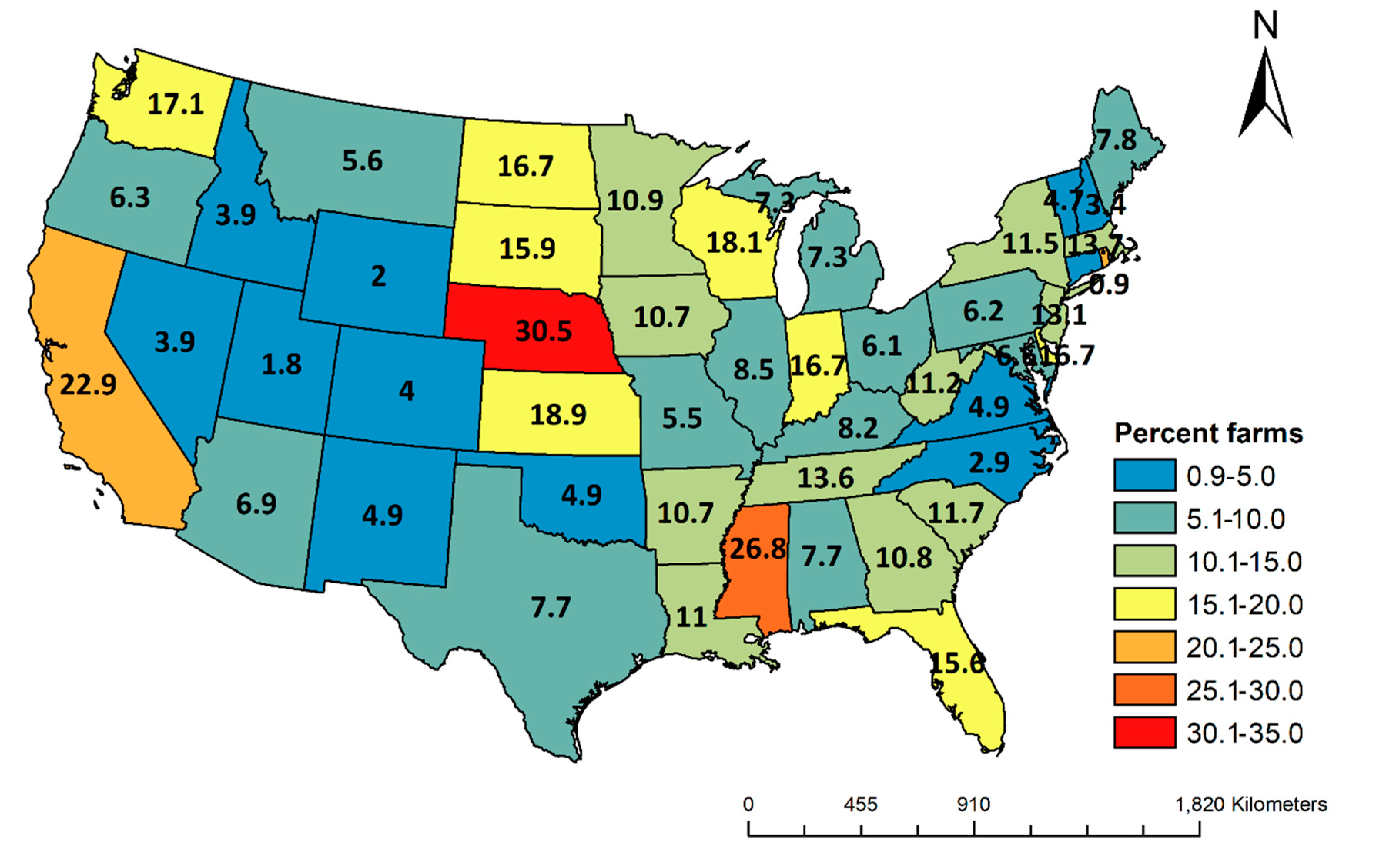
During the recent past, irrigators have shown a moderate level of adoption rates for these technologies in the United States and even lower adoption rates globally. For example, as of 2013, 30.5% of farms in Nebraska used soil moisture sensing devices as their method of irrigation scheduling [17]. This method, while scientifically accepted by substantial research, is also equally or more practical than other available technology-based methods, which include plant moisture sensing devices, crop evapotranspiration (ET_c) reports, computer simulation models and commercial or government scheduling services, as well as non-technology-based methods such as condition of crop, feel of soil, personal calendar schedule, neighbor irrigation-based, etc. [17]. At 30.5%, Nebraska leads the nation in the adoption of soil moisture sensing devices (see Figure 1) and has demonstrated exceptional stewardship in agricultural water management. This has been possible, in part, through efforts of the scientific extension activities and support provided to the stakeholders, e.g., Nebraska Agricultural Water Management Network (NAWMN; https://water.unl.edu/category/nawmn) [18]. The network disseminates advanced farm-scale water management technologies, including soil moisture sensing-based irrigation scheduling to about 1500 collaborators. One of the key emphases of such programs is to increase the adoption rates of technology by producers and their advisors, crop consultants, and other stakeholders. Despite the encouraging success of soil moisture sensing adoption, there still remains immense potential that has to be tapped if the challenge of producing more crop yield from increasingly limited freshwater resources is to be met in the future. In the United States, 11.2% of the farms use soil moisture sensing devices [17], which shows the substantial untapped potential to improve agricultural water use and management.

One of the significant challenges in irrigated/water management is the fact that approximately 9 in 10 farms in the United States are currently not using science-based practical tools for irrigation management decision-making, which raises concerns about the effectiveness of supportive research and outreach in the domain of technology adoption. We hypothesize that a significant hindrance to soil moisture sensor adoption is the lack of a well-defined guide to aid users in understanding and prioritizing their expectations from technology. Selection is especially problematic when there is a multitude of sensor variants available that rely on varying principles and hence are subject to varying uncertainties when employed in different soil textures. The suitability of a sensor, when directed towards adoption by various user groups, is an important aspect of the sensor selection process, but one that has been overlooked in most, if not all, of the research conducted in this direction. While almost the entirety of the literature discusses sensor performance accuracy as the sole criterion for the sensor selection process, we argue that operational feasibility plays a significant role, in addition to performance accuracy, and should be emphasized. Operational feasibility can include monetary and logistical features associated with the sensor that lead to preferential selection of one sensor over another. Although performance accuracy is the foremost concern for scientific users, commercial agricultural users often prioritize operational feasibility that includes monetary aspects, ease of operation, durability, labor, management, etc. For instance, a commercial production field with high soil spatial variability entails that soil moisture be measured at numerous sites, requiring substantial investment in sensors and their connectivity. In addition, it would be a labor-intensive task for the irrigation manager to retrieve and analyze and interpret soil moisture data from these sites frequently to carry out decision-making. Time, cost, and labor are crucial inputs in any commercial operation, underscoring the importance of operational feasibility of soil moisture, in addition to performance accuracy. This research aims to fill a significant knowledge gap in the area of consideration of operational feasibility of soil moisture sensing technology, which has not received any emphasis in the past.

The overall goal of this research is to develop, evaluate, and propose a framework that can comprehensively evaluate soil moisture sensors with respect to: (a) performance accuracy; and (b) operational feasibility. These evaluations were conducted for nine commercially available sensors [TrueTDR-315L (Acclima, Inc., Meridian, ID), CS616 and CS655 (Campbell Scientific, Inc., Logan, UT), 5TE, 10HS, EC-5 and MPS-6 (Meter Group, Pullman, WA), SM150 (Delta-T Devices Ltd., Cambridge, UK) and John Deere Field Connect (John Deere Water, San Marcos, Cal.)] under silt loam and loamy sand soils for two different installation orientations [sensing component parallel (horizontal) and perpendicular (vertical) to the ground surface] typically used. A decision-making guide is proposed that will aid in the selection of the best sensor, both performance-wise and feasibility-wise, under different conditions of use by a large spectrum of users.

2. Materials and Methods

2.1. Description of Soils, Vegetative Characteristics, and Management at the Experimental Sites

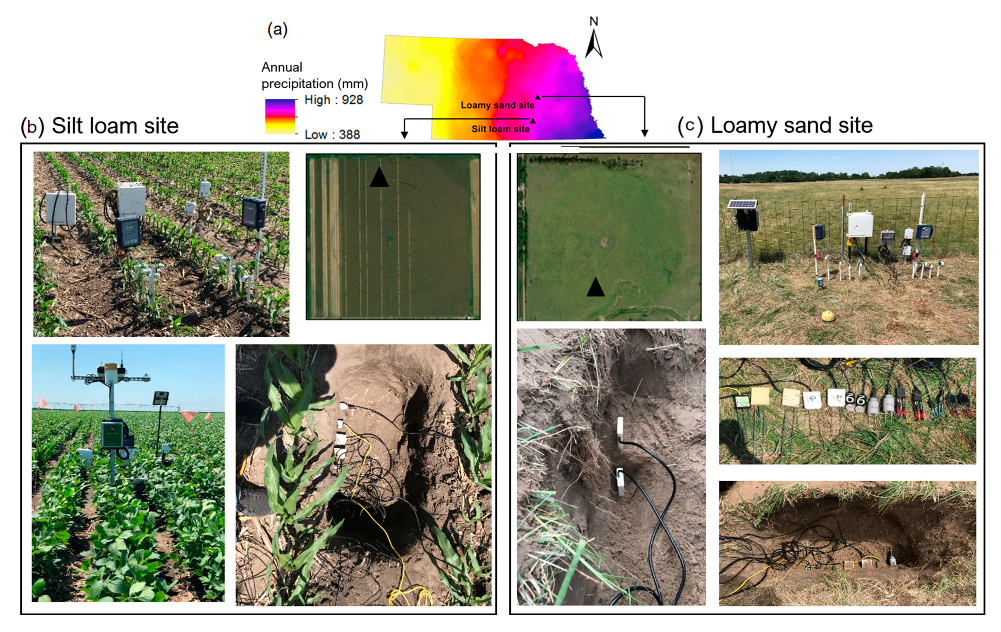
Two dominant soil types in Nebraska were selected for the field experiments, which were carried out in the 2017 and 2018 growing seasons. Hereon, we will refer to Site 1 and Site 2 (Figure 2) by their soil types, i.e., silt loam and loamy sand, respectively.

Silt loam (Site 1): The first experimental site (Site 1) was at the University of Nebraska-Lincoln South Central Agricultural Laboratory (SCAL) (40° 43′ N and 98°8′ W at an elevation of 552 m above mean sea level), near Clay Center, Nebraska. The long-term average annual precipitation in this area is 730 mm and the long-term average growing season (May 1—September 30) precipitation is 437 mm. This site has well-drained Hastings silt loam soil (Crete fine, smectitic, mesic Pachic Argiustolls) with field capacity (FC) and permanent wilting point (PWP) of 0.34 m³ m⁻³ and 0.14 m³ m⁻³, respectively. Irrigated row crops were grown during the experimental period. Field maize (Zea mays L.) and soybean (Glycine max) were grown in 2017 and 2018, respectively. Typical effective rooting depth of field maize and soybean at the experimental site is 1.20 m and 0.90 m, respectively. Total available water holding capacity of the top 1.50 m soil profile is approximately 300 mm. The experimental field (16.5 ha) was irrigated using a four-span hydraulic and continuous-move center-pivot irrigation system (T-L Irrigation, Hastings, Nebraska). Irrigation management was conducted to maintain crops at optimum growth conditions and maintain soil-water near 40%–45% of maximum allowable depletion. The irrigation amount applied was 159 mm in 2017 and 64 mm in 2018.

Loamy sand (Site 2): The second experimental site (Site 2) was at Central City, (41°16′ N 97°56′ W at an elevation of 549 m above mean sea level) approximately 10 km north of the Platte River, Nebraska. Here, the long-term average annual and growing season precipitation is 732 mm and 464 mm, respectively. This site has deep, moderately drained, and moderately permeable loamy sand (Ipage mixed, mesic, Oxyaquic Ustipsamments) with a FC and PWP of 0.19 m³ m⁻³, and 0.05 m³ m⁻³, respectively. This site was a rainfed native grassland approximately 70 ha in size and contains primarily buffalograss [Bouteloua dactyloides (Nutt.)] (∼90%) and tall fescue (Festuca arundinacea). This grassland was established in 1980 and still maintains its natural establishment conditions. Due to rainfed conditions, the vegetation experiences water stress, especially during July and August. It is grazed throughout most of the growing season, and the grass height varies between approximately 5 and 13 cm throughout the season [19]. Nebraska has approximately 19.6 million ha of land that comprises approximately 12 million ha of grassland (rangeland), 1.9 million ha of irrigated maize, and 0.8 million ha of irrigated soybean [19]. Thus, the vegetative surfaces in these experiments are well representative of Nebraska and the Midwestern region and many other parts of the US and world, and hence hold significance for the state and other states and locations of the world with similar soil characteristics and cropping systems.

Table 1. Measured physical, hydraulic, and chemical properties of the two experimental soils.

Soil Type	Soil Layer (cm)	Particle Size Distribution			ρb 1	OMC 2	FC 3	PWP 4	Saturation	Slope	Comp 5	EC 6
		(%) Sand	(%) Silt	(%) Clay	(g cm−3)	(%)	(m3 m−3)	(m3 m−3)	(m3 m−3)	(%)	kPa	dS/m
Silt Loam	0–30	18.7	55.6	25.6	1.35	2.81	0.34	0.17	0.50	0	0.90	0.35
	30–60	16.2	45.3	38.5		2	0.38	0.23	0.50
	60–90	15.8	51	33.2		1.3	0.36	0.20	0.47
	90–120	15.8	56.1	28.1		1.07	0.35	0.17	0.46
Loamy Sand	0–120	77	16	7	1.54	1.1	0.19	0.05	0.42	1.0	0.96	0.13
Soil Type	pH	N	P	K	Ca	Mg	Na	Zn	Fe	Mn	Cu	CEC	SAR
	ppm
Silt Loam	5.8	25.7	33	528	1950	321	45	2.5	64.8	12.4	0.5	19	0.83
Loamy Sand	6.4	12.3	14	172	1140	206	57	0.7	32.7	3.7	0.4	8.1	1.09

¹ ρ_b: bulk density; ² OMC: organic matter content. ³ FC: field capacity; ⁴ PWP: permanent wilting point. ⁵ Comp: compaction. ⁶ EC: electrical conductivity.

presents some of the measured basic soil characteristics at both sites. The inclusion of these two soil types for our experiments provides an opportunity to evaluate the sensors for use in conditions representative of irrigated and rainfed agricultural production systems.

2.2. Soil Moisture Sensors Investigated

We used nine different commercial soil moisture sensors in our evaluations that fall into three main categories when classified by operational principles. At each site, we evaluated two sets of each sensor, one of which was installed in horizontal (parallel to the ground surface) orientation and the other in vertical (perpendicular to the ground surface) orientation. The only exceptions were the JD multi-sensor probe, which can only be installed vertically and TDR315L (Acclima), which was only evaluated in horizontal orientation. Following are all the sensors included in this research under their corresponding principles of operations:

Time-Domain Reflectometry (TDR)-based Sensors

• TrueTDR-315L Acclima (Acclima, Inc., Meridian, ID)
• CS616 (Campbell Scientific, Inc., Logan, UT)
• CS655 (Campbell Scientific, Inc., Logan, UT)

Capacitance-based Sensors

• 5TE (Meter Group, Pullman, WA)
• 10HS (Meter Group, Pullman, WA)
• EC-5 (Meter Group, Pullman, WA)
• SM150 (Delta-T Devices, Cambridge, U.K.)
• John Deere (JD) Field Connect (John Deere Water, San Marcos, Cal.)
• Dielectric Water Potential-based SensorTEROS 21 (MPS-6) (Meter Group, Pullman, WA)

All sensors report soil moisture status as volumetric water content (θ_v) (m³ m⁻³% vol), except TEROS 21 (MPS-6), which reports soil matrix potential (Ψ_m) (kPa). We converted each soil layer’s Ψ_m measurements to θ_v using soil-specific soil-water release curves developed by [20].

2.3. Reference (True) Moisture Measurement

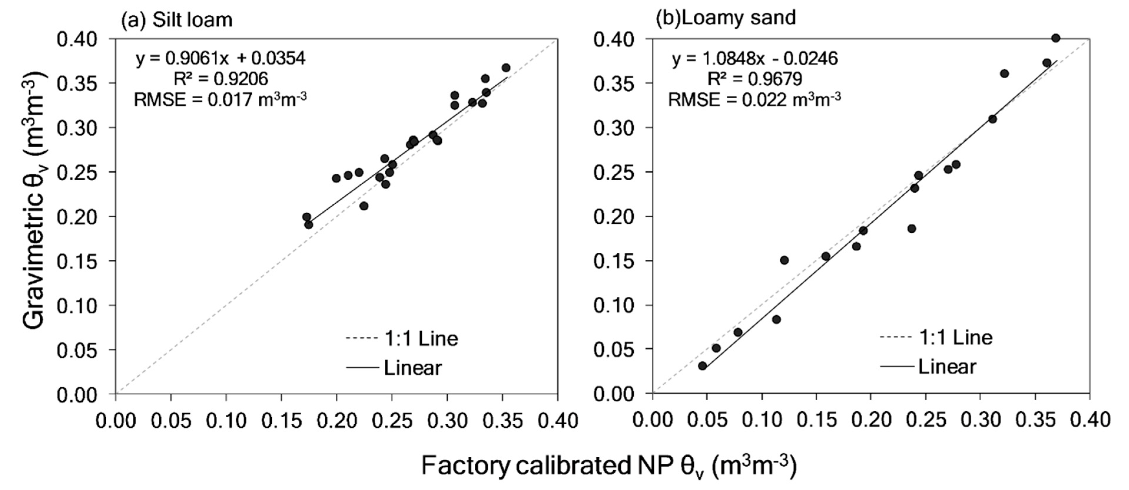
We used a new Troxler Model 4302 neutron probe (NP) soil moisture gauge (Troxler Electronic Laboratories, Inc., Research Triangle Park, N.C.) to represent true θ_v (θ_vref) information in our research. All other sensors in question have been compared, assessed, and calibrated against NP measurements. For accurate soil moisture measurements, site-specific calibration equations were developed [20] for both sites by correlating the factory-calibrated NP measurements to the gravimetric-sample-determined θ_v (Figure 3; Equations (1) and (2)).

Silt Loam:

$$\mathrm{y}=0.9061\mathrm{x}+0.0354$$

(1)

Loamy Sand:

$$\mathrm{y}=1.0848\mathrm{x}-0.0246$$

(2)

where, y refers to factory calibration θ_vref, and x refers to gravimetric θ_v.

Two NP access tubes were installed at each of the sites for reference (true) soil moisture information. These tubes were installed in very close vicinity of the sampling area of the sensors to be evaluated. For example, in silt loam, NP access tubes were installed in the inter-plant spacing in the same row as other sensors, ensuring fair evaluation (the row spacing in the silt loam soil-Site 1 was 0.76 m for maize and soybean). The access tubes were covered at all times, except when measuring soil moisture, to avoid any interaction with ambient moisture conditions (rainfall, irrigation, dew formation, etc.).

2.4. Installation Specifications

We investigated all the sensors that can be installed in varying orientations under two orientations (vertical and horizontal). Hereon, the four different soil type-orientation combinations are referred to as silt loam H (for horizontal), silt loam V (for vertical), loamy sand H, and loamy sand V. Soil profiles (pits) were dug at both sites for horizontal sensor orientation so that the four boundary walls of the pits were perpendicular to the pit bottom plane. The soil beyond the cuboidal pit was ensured to be undisturbed and soil structure was maintained. In silt loam soil, the pit was dug in the furrow, whereas in loamy sand soil, the pit was dug in a representative grassed area. For horizontal orientation (silt loam H and loamy sand H), the sensors were installed parallel to the ground surface against one of the pit walls at 60 cm depth from soil surface, such that the sensing components of the sensor (prongs, ceramic disks, etc.) resided in undisturbed soil and sampled soil moisture in undisturbed soil. Sensor outputs are highly sensitive to the effectiveness of sensor installation, requiring that extreme caution is used in the installation procedure. The inter-sensor distance was kept such that volumes (area) of influence of various sensors are independent. Post-installation, the pit was refilled with the same volume of soil, compacted to original conditions) and the same soil layers were placed back in their original depths to enable the construction of the original soil layers.

For vertical orientation (silt loam V and loamy sand V), the sensors were installed perpendicular to the ground surface, such that the sensing components were placed in undisturbed soil. The vertical sensors were oriented so that the geometrical midpoints of the sensing components lie on the same horizontal plane, ensuring fair comparisons across sensors with variable sensing volumes. For silt loam V, the horizontal plane was at 30 cm from the ground surface, while for loamy sand V, it was 50 cm from the ground surface. For silt loam site H, the sensors were installed directly under the plant row within the root zone; and for silt loam V, they were installed in the inter-plant spacing, ensuring sampling of the root zone.

The JD probe, being a multidepth probe had different installation specifications than those discussed above. JD probes can only be vertically installed perpendicular to the ground, and hence, we were not concerned with installation orientations in this case. The JD probes were compared to NP soil moisture measurements at five different depths where the capacitors are placed, i.e., 10, 20, 30, 50, and 100 cm. While these depths are alterable, manufacturer default depths were used in this research.

2.5. Soil Mositure Data Measurement and Retrieval

All the sensors in question were equipped with various manufacturer-recommended dataloggers that read soil moisture status every minute and output hourly averages throughout the two growing seasons. The datasets were retrieved manually, except for the JD probe, for which telemetry was used for data retrieval. The NP measurements were conducted at both access tubes at the two sites every week throughout the two growing seasons. At each access tube, eight neutron count measurements were conducted each week, each corresponding to the depths where various sensors were installed, i.e., 10 cm (JD probe), 20 cm (JD probe), 30 cm (JD probe and all sensors under silt loam V), 50 cm (JD probe and all sensors under loamy sand V), 60 cm (for all sensors under silt loam H and loamy sand H), 90 cm [(for all sensors under loamy sand and silt loam (both H and V)], 100 cm (JD probe) and 120 cm [for all sensors under loamy sand and silt loam (both H and V)].

2.6. Statistical Analysis

All sensors were evaluated for their performance in estimating θ_v accurately using root mean squared error (RMSE, m³ m⁻³), computed as described in Equation (3).

$$\mathrm{RMSE}=\sqrt{\frac{{{\displaystyle \sum }}_{\mathrm{i}=1}^{\mathrm{n}}{\left({\mathrm{E}}_{\mathrm{i}}-{\mathrm{M}}_{\mathrm{i}}\right)}^2}{\mathrm{n}}}$$

(3)

where, M_i is sensor-computed variables, E_i is corresponding NP-measured (true) variables, and n is number of observations. RMSE was used to denote the absolute value of the error that would be associated with these sensor-estimated variables, if the sensor in question is used to report soil moisture status, as calculated from the experimental data.

2.7. Evaluation Metrics

Each sensor included in this research was subject to evaluation for two major characteristics that are expected from an ideal sensor used for agricultural irrigation management by any user. These characteristics were: (i) operational feasibility; and (ii) performance accuracy. The following sections describe the methodology adopted in this research to address the suitability of the sensors under these criteria.

2.7.1. Operational Feasibility

The definition of operational feasibility in this research includes four characteristics that an ideal sensor is expected to possess. These are: (a) telemetry; (b) sensor cost; (c) data logging cost; and (d) ease of operation. A detailed description of each of these factors as well as how they were addressed in a quantitative framework is presented in the following sections.

Telemetry

Telemetry (TM) is referred to as the ability to have near-real-time access to the data that is collected at the monitoring site. The moisture data is usually made available in the web platform and can be accessed through a cell phone, iPad, and other devices. The data transmittal is achieved via terrestrial radio or satellite systems, and usually a wireless cost is incurred that could be a fixed cost or can vary with per unit of data transfer. Solar panels are usually employed to generate electrical power; hence, the data collection and transfer is independent of the power grid. A soil moisture sensor system equipped with TM options provides the user with the ability to monitor the soil profile for available water in near-real time, and prevents the time and labor investment to physically visit the monitoring site repeatedly. Moreover, it could also prevent risky situations where the moisture levels are close to the irrigation trigger, and the user does not have access to the data, given time and labor constraints. Generally, most of the sensors available currently have some provision of being equipped with a telemetric system with an associated cost. Typically, on a commercial level, this is accomplished either by adding a TM module to an existing datalogger, or by using a datalogger with built-in telemetry provision.

In this research, we converted the qualitative information of availability or nonavailability of TM to a quantifiable metric, to which we refer to as Score 1, and is determined using the following equation:

$$\mathrm{Score}1=\{\begin{array}{c}0 \mathrm{if} \mathrm{no} \mathrm{provision} \mathrm{of} \mathrm{telemetry}\\ 100 \mathrm{if} \mathrm{telemetric} \mathrm{provision} \mathrm{exists}\end{array}$$

(4)

Sensor Cost

The cost of the sensing device is a very important factor for consideration, especially for a commercial producer, to consider in the selection criteria. The cost of each sensor included in this research was enquired from the respective manufacturers, and the costs (

Table 2. Cost of sensor and sensor and datalogger [with and without telemetry (TM)] used in the deduction of scores. The prices are in US Dollars and reflect the prices obtained from the manufacturers that were in effect as on 13 March 2019.

Sensor	Sensor Cost ($)	Sensing and Logging Cost ($) (No TM)	Sensing and Logging Cost ($) (TM)
CS655	228	1928	2378
CS616	148	1848	2298
SM150	230	1590	3590
10HS	128	624	1274
EC-5	120	616	1266
5TE	225	721	1371
TEROS 21 (MPS-6)	225	721	1371
JD Probe	193	1193	2193
TDR315L (Acclima)	295	670	N/A 7

N/A: not available either from manufacturer or our research data.

) represent those effective on March 13, 2019, and are subjected to change with time. However, the relative magnitudes of the costs will remain equivalent to what is reported in this research, and, hence, our findings will hold true.

It is crucial to rescale the absolute sensor costs to a scale of 0–100 in order to be consistent with the other factor-specific scores that we have quantified. The score for sensor cost is referred to as Score 2, and is calculated using the following equation:

$$\mathrm{Score}2=100-\left(\frac{{\mathrm{Max}}_{\mathrm{scaled}}-{\mathrm{Min}}_{\mathrm{scaled}}}{{\mathrm{Max}}_{\mathrm{cost}}-{\mathrm{Min}}_{\mathrm{cost}}}\right)\times \left(\mathrm{Sensor}\mathrm{cost}-{\mathrm{Min}}_{\mathrm{cost}}\right)+{\mathrm{Min}}_{\mathrm{scaled}}$$

(5)

where, Max_scaled and Min_scaled are the extremes of the scale of the score metric, i.e., 0 and 100, Max_cost and Min_cost are the extremes of the scale of the absolute sensor cost (US dollar amount in Table 2), sensor cost is the dollar amount of the cost of the sensor for which Score 2 is calculated. Thus, using this scaling technique, the sensor that is the cheapest in the complete sensor panel is assigned a Score 2 of 100; and the costliest sensor is assigned a Score 2 of 0. All other sensors were assigned accordingly within this scale of 0 to 100.

Sensing and Logging Cost

Effective and accurate sensing and datalogging of soil moisture data constitutes important consideration in cost. Operational use of a soil moisture sensing device for irrigation management in a commercial field entails that the data are logged at fixed intervals, typically at 30–60 min intervals. This is advantageous for three major reasons: (i) having a representative daily soil moisture status independent of diurnal variations; (ii) access to historical data for retrospection in decision-making; and (iii) access to historical data for scrutiny for data quality assurance in case of sensor malfunction or due to other sources of error. Thus, in the majority of cases, the total incurred cost by the user will include both sensing and data logging (DL) cost (Equation (6)). Further, this cost will depend on whether or not the sensing operation includes TM (Equation (7)).

$${\mathrm{Total}\mathrm{Cost}}_{\mathrm{No}\mathrm{TM}}=\mathrm{Sensor}\mathrm{Cost}+\mathrm{DL}\mathrm{cost}$$

(6)

$${\mathrm{Total}\mathrm{Cost}}_{\mathrm{TM}}=\mathrm{Per}\mathrm{sensor}\mathrm{cost}+\mathrm{DL}\mathrm{cost}+\mathrm{TM}\cos \mathrm{t}$$

(7)

Following the computation of the total cost (Table 2), the total cost was rescaled as Score 3, using a method parallel to the one used when computing Score 2, and is indicated by Equation (8):

$$S\mathrm{core}3=100-\left(\frac{{\mathrm{Max}}_{\mathrm{scaled}}-{\mathrm{Min}}_{\mathrm{scaled}}}{{\mathrm{Max}}_{\mathrm{Total}\cos \mathrm{t}}-{\mathrm{Min}}_{\mathrm{Total}\mathrm{cost}}}\right)\times \left(\mathrm{Total}\mathrm{cost}-{\mathrm{Min}}_{\mathrm{Total}\mathrm{cost}}\right)+{\mathrm{Min}}_{\mathrm{scaled}}$$

(8)

where, Max_scaled and Min_scaled are the extremes of the scale of the score metric, i.e., 0 and 100, Max_{Total cost} and Min_{Total cost} are the extremes of the scale of the absolute total cost (dollar amount in Table 2), Total cost is the dollar amount of the cost of the sensor and datalogger (and TM, if desired) for which Score 3 is calculated (using Equations (6) or (7), whichever is applicable). Thus, using this scaling method, the sensor package (Sensor + DL + TM) that is the cheapest in the complete sensor panel is assigned a Score 3 of 100; and the costliest sensor package is assigned a Score 3 of 0. All other sensors are assigned accordingly within this scale of 0 to 100.

Ease of Operation

This factor is a highly subjective factor that addresses the degree of ease of various interactions of the user with the sensor package at various stages. These stages include any potential programming (or setting up) of a datalogger, data retrieval from a datalogger, and data post-processing that is required prior to data use for decision-making. The evaluation for this factor in each sensor was reflected by Score 4, which was based on: (i) whether the datalogger associated with a graphical user interface (GUI); and (ii) whether any post-processing on the sensor data was necessary. Dataloggers which have a GUI when used with a computer are considerably easier to set up and more user-friendly than others that require programming skills (CR10X datalogger for CS616 and CS655 requires programming in Visual Basic). Any data post-processing that is required in a given sensor package is a reason for avoidable delay before actual decision-making. For example, TEROS21 (MPS-6) output data are in units of soil matric potential (kPa), rather than volumetric water content (m³ m⁻³). This necessitates conversion of kPa to m³ m⁻³, which requires careful laboratory-based development of soil–water retention curves, causing additional costs. The following equation (Equation (9)) represents our methodology of assigning a quantifiable score from the qualitative information discussed above:

$$\mathrm{Score}4=\{\begin{array}{c}0 \mathrm{if} \mathrm{no} \mathrm{GUI}\\ 100 \mathrm{if} \mathrm{GUI} \mathrm{available}, \mathrm{no} \mathrm{data} \mathrm{post} \mathrm{processing}\\ 50 \mathrm{if} \mathrm{GUI} \mathrm{available}, \mathrm{require} \mathrm{data} \mathrm{post} \mathrm{processing}\\ 1\end{array}$$

(9)

It has to be noted that all of the sensor-specific scores developed under operational feasibility (Scores 1, 2, 3, 4) are common for any soil conditions and sensor orientations. Moreover, they are also unaltered, whether factory calibrations (F.C.) or site-specific calibrations (S.S.C.) are used.

2.7.2. Performance Accuracy

The performance accuracy metric quantifies the success of a sensor to reflect accurate soil moisture status under a given set of soil type (silt loam and loamy sand), orientation (H or V), and calibration (F.C. or S.S.C.). Unlike operational feasibility features, the performance accuracy is specific to a particular soil type and orientation the sensor is installed in. For each soil type-orientation combination (silt loam H, silt loam V, loamy sand H, and loamy sand V), root mean squared error (RMSE) for each sensor’s volumetric water content θ_v (m³ m⁻³) against reference neutron scattering-measured θ_v was calculated. Moreover, RMSE obtained under both F.C. and S.S.C. were used in this research.

It is necessary that the RMSE statistic be converted to a scale that is consistent to that of operational feasibility metrics, i.e., score on a scale of 0–100. We refer to this as the performance accuracy (P.A.) score and is computed using the following rescaling equation:

$$\mathrm{P}.\mathrm{A}.\mathrm{score}=100-\left(\frac{{\mathrm{Max}}_{\mathrm{scaled}}-{\mathrm{Min}}_{\mathrm{scaled}}}{{\mathrm{Max}}_{\mathrm{RMSE}}-{\mathrm{Min}}_{\mathrm{RMSE}}}\right)\times \left(\mathrm{RMSE}-{\mathrm{Min}}_{\mathrm{RMSE}}\right)+{\mathrm{Min}}_{\mathrm{scaled}}$$

(10)

where, Max_scaled and Min_scaled are the extremes of the scale of the score metric, i.e., 0 and 100, Max_RMSE and Min_RMSE are the extremes of the scale of the sensor-specific RMSE in different soil type, orientation, and calibration combination (

Table 3. Root mean squared error (RMSE) in m³ m⁻³ for each sensor under the two soil types, two orientations, and two calibration types.

Soil Type	Sensor	RMSE (m3 m−3)
		Vertical		Horizontal
		F.C. 8	S.S.C. 9	F.C.	S.S.C.
Silt Loam	CS655	0.05	0.03	0.15	0.05
	CS616	0.06	0.03	0.40	0.05
	SM150	0.07	0.02	0.06	0.04
	10HS	0.10	0.03	0.07	0.06
	EC-5	0.15	0.03	0.15	N/A 10
	5TE	0.05	0.02	0.06	0.04
	TEROS 21 (MPS-6)	0.08	0.03	0.11	0.05
	JD Probe	0.05	0.06	N/A	N/A
	TDR315L (Acclima)	N/A	N/A	0.06	0.04
Loamy Sand	CS655	0.03	0.03	0.01	0.02
	CS616	0.03	0.02	0.03	0.02
	SM150	0.04	0.04	0.02	0.02
	10HS	0.04	0.02	0.14	0.02
	EC-5	0.05	0.04	0.09	0.02
	5TE	0.04	0.04	0.03	0.01
	TEROS 21 (MPS-6)	0.21	0.03	0.22	N/A
	JD Probe	0.01	0.02	N/A	N/A
	TDR315L (Acclima)	N/A	N/A	0.02	0.02

⁸ F.C.: factory calibration; ⁹ S.S.C.: site-specific calibration; ¹⁰ N/A: not available either from manufacturer or in our research data.

), RMSE is the root mean squared error for a sensor under a certain soil type, orientation, and calibration combination for which a P.A. score is calculated. Thus, using this scaling technique, the sensor that is the most accurate in the complete sensor panel is assigned a P.A. score of 100; and the least accurate sensor is assigned a P.A. score of 0. All other sensors are assigned scores accordingly within this scale of 0 to 100.

3. Results and Discussion

3.1. Assessment of Sensor-Specific Operational Feasibility Score

The algorithms presented earlier (equations 4, 5, 8, 9) were used to compute scores 1, 2,3, 4 for each sensor to represent their evaluation for telemetry, sensor cost, sensing and logging cost (with TM and no TM), and ease of operation, respectively. All sensors performed equally when evaluated for TM availability, and had Score 1 of 100 (

Table 4. Scores calculated for various operational feasibility (O.F.) factors and performance accuracy (P.A.) for each sensor. The O.F. scores are universal, whereas P.A. score varies with soil types, installation orientations, and calibration types.

	Operational Feasibility (O.F.) Score					Performance Accuracy (P.A.) Score
Column ID	1	2	3	4	5	6
Sensor	Score 1	Score 2	Score 3 (Non-TM)	Score 3 (TM)	Score 4	Silt Loam V		Silt Loam H		Loamy Sand V		Loamy Sand H
						F.C. 11	S.S.C. 12	F.C.	S.S.C.	F.C.	S.S.C.	F.C.	S.S.C.
CS655	100	38	0	52	0	100	76	73	47	90	66	100	53
CS616	100	84	6	56	0	87	80	0	31	94	74	95	79
SM150	100	37	26	0	100	74	100	100	80	85	0	98	0
10HS	100	95	99	100	100	44	84	95	2	87	100	41	8
EC-5	100	100	100	100	100	0	75	73	N/A	84	17	65	84
5TE	100	40	92	95	100	97	94	100	100	87	11	91	100
TEROS 21 (MPS-6)	100	40	92	95	50	67	80	85	72	0	23	0	N/A
JD Probe	100	58	N/A 13	60	100	99	0	N/A	N/A	100	81	N/A	N/A
TDR315L (Acclima)	0	0	96	N/A	100	N/A	N/A	98	83	N/A	N/A	97	8

¹¹ F.C.: factory calibration; ¹² S.S.C.: site-specific calibration; ¹³ N/A: not available either from manufacturer or from our research data.

, col. 1), with the exception of TDR-315L (Acclima), for which TM was not available, and hence was assigned a Score 1 of 0.

The sensor cost was the lowest and highest for EC-5 and TDR-315L (Acclima) sensors. In other words, they were the best and the worst sensors cost-wise, and hence were assigned a Score 2 of 100 and 0 (Table 4, column 2), respectively. However, there was not much difference ($225–$230) among sensing costs of CS655, SM150, 5TE, TEROS 21 (MPS-6) (Table 2). These comparatively similar costs were also reflected in the Score 2 assigned to these sensors, which was in the range of 37–40. Unlike Score 1, Score 2 showed greater variability across sensors, and hence would contribute in a crucial fashion to the sensor selection process. As mentioned earlier, sensor cost is one of the most fundamental factors that governs sensor selection by a commercial grower, especially if the target field has considerable soil spatial variability. A multiplier (number of sensors to be installed) can be used to upscale the sensor cost in such a situation. Score 1 is relatively more useful for research and scientific applications, where numerous sensors are required to monitor experimental field plots and greenhouse pots, and the user might not be interested in logging the data, given sufficient labor and time to manually read and record the data.

In practical (and commercial) situations, sensing and logging cost will be the actual total cost incurred by the user. Further, depending on the desire of a user for a TM connectivity, the cost can vary accordingly. Thus, we present Score 3 under two scenarios, i.e., non-TM sensing and datalogging and sensing and datalogging with TM, and are conveyed in Table 4, col. 3 and col. 4, respectively. For non-TM sensing and logging, EC-5 and CS655 scored the highest (100) and the lowest (0), respectively, while for sensing and datalogging with TM, EC-5 and SM150 scored the highest and the lowest, respectively. It was observed that, in most cases, telemetry option affects the total cost and so, can be the priority of the sensor selection. Score 3 also shows substantial variability across sensors, and thus governs the selection to a considerable degree, similar to Score 2. It has to be noted that Score 3 represents the cost for a single sensor and datalogger. In certain cases, the datalogger allows for integration of multiple sensors (EM-50; CR10X; DL-6), and in such cases, the total cost would be readjusted.

Lastly, ease of operation, as assessed by Score 4 (Table 4, col. 5), revealed that all sensors were optimal on this frontier (score of 100), except CS616, CS655, and TEROS 21 (MPS-6). Both CS616 and CS655, since being associated with the CR10X datalogger, which requires programming skills to set them up, to read and record the data, were assigned a Score 4 of 0. TEROS 21, due to the requirement of data post-processing (conversion from kPa to m³ m⁻³), was assigned a Score 4 of 50 (see Equation (9)). These requirements for the use of these sensors present challenges, especially when commercial production is the area of sensor use.

3.2. Performance Accuracy Score

Performance accuracy (P.A.) scores are presented in column 6 in Table 4, individually for silt loam and loamy sand soils under vertical and horizontal orientations when used with field calibration (F.C.) and site-specific calibration (S.S.C.). P.A. scores were computed for each sensor using Equation (10), using sensor-specific RMSE. P.A. scores are site-specific, orientation-specific, and calibration type-specific, and are studied individually for each of these scenarios.

It was found that, for silt loam V under F.C., CS655 and EC-5 had highest and lowest P.A. scores, respectively, due to their low and RMSE values. Lowest RMSE implies highest P.A. score, and vice versa. For silt loam V under S.S.C., SM150 and JD Probe scored the highest and lowest, respectively. It is interesting to note that how using S.S.C. rather than F.C. alters the best and worst choices of sensors. This is because some sensors perform reasonably under F.C. and do not necessarily require a S.S.C. This implies that the sensor selection process has to respect the fact that whether the sensor will be used with a certain S.S.C., as a part of a research and outreach program. This information about calibration-specific uncertainties in soil moisture measurement has been generated through extensive datasets collected through field research for sensor-measured and actual soil moisture over two years.

Similarly, for silt loam H under F.C., 5TE and SM150 scored the highest and CS616 the lowest, while silt loam H under S.S.C., 5TE and 10 HS scored the highest and the lowest, respectively. Overall, it can be observed that, among all sensors, 5TE performed the best under all orientation and calibration-type combinations in silt loam soil when P.A. score was considered (P.A. score was at least 94), implying that it can be well suited for irrigation management and soil water status monitoring in silt loam soils. Nevertheless, we recommend that the users should identify the best sensor given their conditions (orientation, calibration type), rather than selecting a sensor across the spectrum.

The best-suited sensors shifted significantly when the soil type was changed. The best sensors, as reported by P.A. scores in loamy sand soil were JD probe (for loamy sand V under F.C.), 10 HS (loamy sand V under S.S.C.), CS655 (loamy sand H under F.C.), and 5TE (loamy sand H under S.S.C.). Since there are no constituent subfactors in P.A., unlike O.F., the P.A. score is the singular score that was used to assess the suitability of sensors when the degree of accuracy associated with the use of a sensor is a priority. However, unlike O.F., P.A. scores are not universal across the conditions in which they are used, and should be selected based on the soil type, sensor orientation, and calibration type for which they are to be deployed.

3.3. Step-By-Step User Guide for Sensor Selection

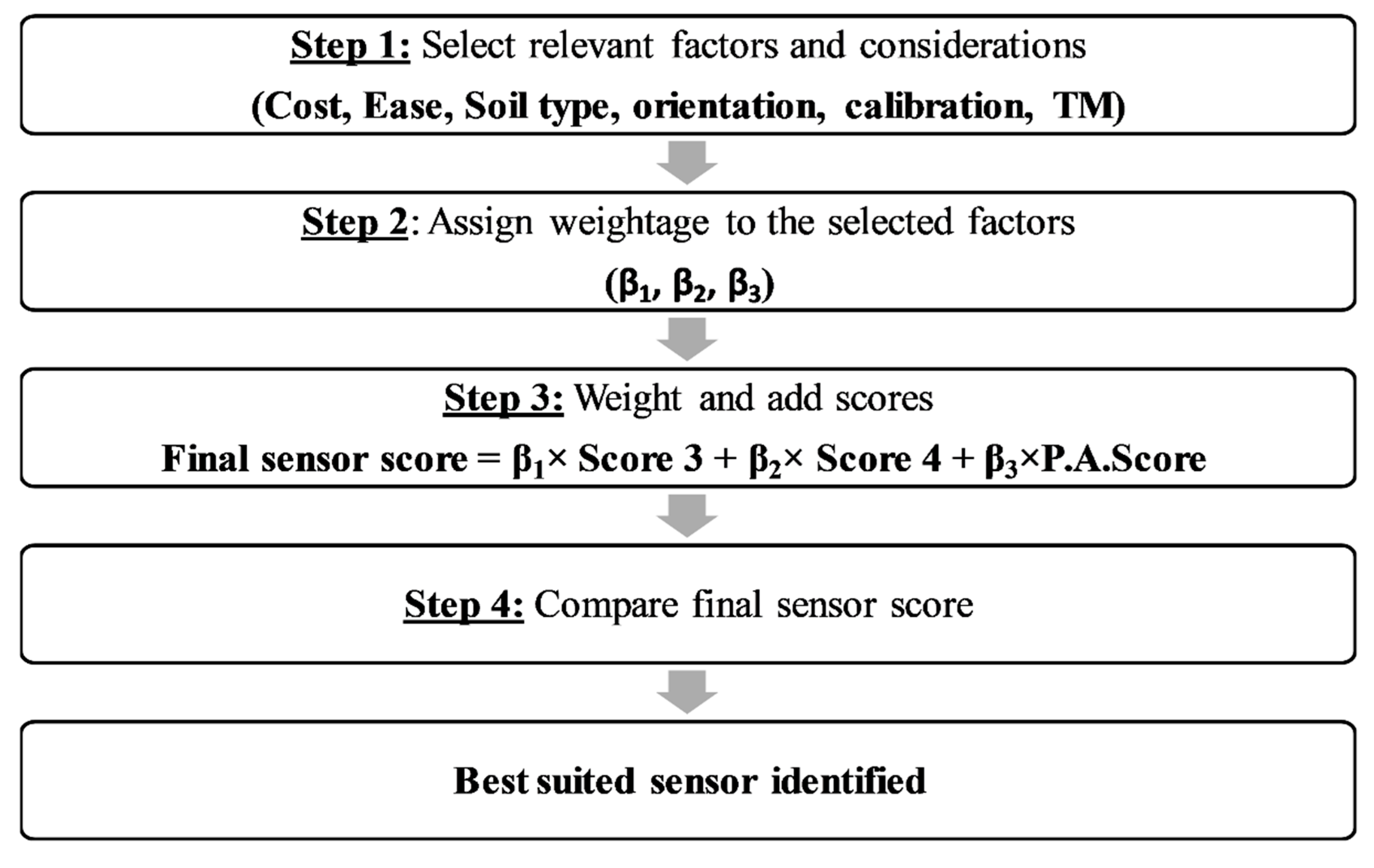
We proposed a framework to aid in sensor selection by a user by developing a methodology to account for various factors that can affect the efficacy or success of a sensor in a given condition (Figure 4). We suggest that the following step-by-step methodology should be followed:

Step 1: Select the factors that are relevant to the user’s situation from the pool of different factors that can be addressed. This includes sensing cost, sensing and datalogging cost (TM or non-TM), ease of operation, which are subfactors under a broad operational feasibility framework, and lastly, performance analysis. The factor selection step aims at recognizing characteristics associated with the sensors that concern the user and can vary widely among different users. For example, if the user is a highly skilled researcher, ease of operation might not be a relevant driver. In such a case, Score 4 can be ignored. On the other hand, if the user is a commercial grower who intends to install a single sensor near the field boundary close to his/her homestead, telemetry costs might not be a concerning factor. In this case, Score 3 (TM) shall be considered. Thus, fulfilling this step would provide clarity on what factors to include in the selection process going forward.

Step 2: Assign desired weightage to each factor, which would also be a function of the intended importance assigned to each factor based on their use. The total weightage (as a fraction of 1) can be divided among the selected factors mentioned in step 1. For example, if the intended use is research, greater weightage can be assigned to P.A. score.

Step 3: Multiply the assigned weightage factor to each score with the corresponding score quantity provided in Table 4. The following equation is used for a situation where sensing and datalogging cost (Score 3), ease of operation (Score 4) and performance accuracy (P.A. score) are weighted by β_1, β₂, and β₃, respectively.

$$\begin{array}{cc}\hfill \mathrm{Final}\mathrm{sensor}\mathrm{score}& \hfill \\ \hfill & ={\mathsf{\beta }}_1\times \mathrm{Score}3\left(\mathrm{either}\mathrm{non}-\mathrm{TM}\mathrm{or}\mathrm{TM}\right)+{\mathsf{\beta }}_2\times \mathrm{Score}4\hfill \\ \hfill & +{\mathsf{\beta }}_3\times \mathrm{P}.\mathrm{A}.\mathrm{Score}\hfill \end{array}$$

(11)

where, final sensor score is the metric compared across the sensors for selection, Scores 3 and 4 are sensor-specific quantities to be used from columns 3 (non-TM)/4 (TM) and 5 from Table 4. β_1, β₂, and β₃ are the weightage factors assigned to sensing and logging cost, ease of operation, and performance accuracy, by the user.

Step 4: Finally, the final sensor score is compared across the sensors to evaluate the relative degree of success and effective operational feasibility expected with the use of the sensors. The sensor for which the final sensor score is the maximum is ideally the best-suited sensor for the intended application.

As a case study to explain this workflow described in the above steps, the entire sensor selection process was carried out under certain example conditions.

Table 5. Case study considerations, step-wise computations, and final sensor selection details for the case study shown.

Case Study Considerations	Soil Type: Silt Loam
	Orientation: Vertical
	Calibration Type: Factory Calibration
	TM: No
Step 1 (Factor selection)	Sensing and logging cost (non-TM)
	Ease of operation
	Performance accuracy
Step 2 (Assign weightage)	β1 = 0.1
	β2 = 0.3
	β3 = 0.6
Step 3 (Add weighted scores)
Step 4 (Compare final sensor scores)	Sensor	β1 × Score 3	β2 × Score 4	β3 × P.A. Score	Final sensor score	Rank
	CS655	0	0	60	60	5
	CS616	1	0	52	53	6
	SM150	3	30	44	77	2
	10HS	10	30	26	66	3
	EC-5	10	30	0	40	7
	5TE	9	30	58	98	1
	TEROS 21 (MPS-6)	9	15	40	64	4
	JD Probe	N/A14	30	59	N/A	N/A
	TDR315L (Acclima)	10	30	N/A	N/A	N/A
	Best-suited sensor: 5TE

¹⁴ N/A: not available either from manufacturer or our research data.

lists the considerations and factors that are relevant in this particular case study and lists the quantities obtained at each step of the guide. This case study acts as an example resource to understand the process of sensor selection that we proposed in this research.

4. Conclusions

This research recognizes the crucial need to emphasize factors that play a significant role in the desirability/selection of soil moisture sensors. These factors elucidate the operational feasibility of nine commercially available soil moisture sensors by identifying and quantifying factors such as cost of sensing, datalogging, telemetry and ease of sensor operation. This was achieved by assessing the abovementioned characteristics in all nine sensors and quantifying scores that ranged from 0 to 100 for each of these governing factors. The operational feasibility of the sensors was merged in conjunction with sensor accuracy. Finally, a step-by-step guide was proposed that aimed at appropriate sensor selection under various expectations, considerations, soil types, orientations and calibration types. We expect the resources in the form of scores and ranks presented here for each sensor to be valuable to a wide community of users, ranging from researchers to commercial growers. In addition to the sensor-specific information and analysis presented here, the conceptual framework of sensor selection presented can be extended to any other soil moisture sensors that are not been included in this research. To the best of our knowledge, this research is the first attempt to address the need of non-sensor-performance-related expectations from a desired sensor in a quantitative fashion.