Article

Density of Biogas Power Plants as An Indicator of Bioenergy Generated Transformation of Agricultural Landscapes

1
Department of Physical Geography and Geoinformatics, University of Szeged, Egyetem u. 2–6, H-6722 Szeged, Hungary
2
Department of Geography, Division of Physical Geography: Landscape Ecology and Geoinformation Science, Center for Geoinformation, Kiel University, D-24098 Kiel, Germany
3
Department of Geography, Division of Physical Geography: Landscape Ecology and Geoinformation Science, Kiel University, D-24098 Kiel, Germany
*
Author to whom correspondence should be addressed.
Sustainability 2019, 11(9), 2500; https://doi.org/10.3390/su11092500
Submission received: 20 March 2019 / Revised: 23 April 2019 / Accepted: 24 April 2019 / Published: 29 April 2019

Abstract

:
The increasing use of biogas, produced from energy crops like silage maize, is supposed to noticeably change the structures and patterns of agricultural landscapes in Europe. The main objective of our study is to quantify this assumed impact of intensive biogas production with the example of an agrarian landscape in Northern Germany. Therefore, we used three different datasets; Corine Land Cover (CLC), local agricultural statistics (Agrar-Struktur-Erhebung, ASE), and data on biogas power plants. Via kernel density analysis, we delineated impact zones which represent different levels of bioenergy-generated transformations of agrarian landscapes. We cross-checked the results by the analyses of the land cover and landscape pattern changes from 2000 to 2012 inside the impact zones. We found significant correlations between the installed electrical capacity (IC) and land cover changes. According to our findings, the landscape pattern of cropland—expressed via landscape metrics (mean patch size (MPS), total edge (TE), mean shape index (MSI), mean fractal dimension index (MFRACT)—increased and that of pastures decreased since the beginning of biogas production. Moreover, our study indicates that the increasing number of biogas power plants in certain areas is accompanied with a continuous reduction in crop diversity and a homogenization of land use in the same areas. We found maximum degrees of land use homogenisation in areas with highest IC. Our results show that a Kernel density map of the IC of biogas power plants might offer a suitable first indicator for monitoring and quantifying landscape change induced by biogas production.

Graphical Abstract

1. Introduction

In order to lower greenhouse gas emissions, the EU member states intend to add an increasing share of renewable energy sources to their national energy systems. Renewable resources like wind, solar, geothermal, hydropower, and biogas produced from biomass allow the generation of electricity and heat, which contributes to reaching the climate protection goals of the European energy sector [1]. Currently, energy from biogas, mostly electricity [2], yields 7.6% of primary renewable energy production in the EU. Biogas produced by anaerobic co-digestion of waste and agricultural products like manure and energy crops contributes 69% to this share [3].
Today, the usage of biogas and biomass to produce electricity is a world-wide applied technology. It is a relevant topic all over the world, as shown by the current studies on sustainable use of crop residues in biogas power plants in the USA [4], the changes in agriculture systems in East European countries [5,6], or analysis of straw and manure potentials as feedstock in China [7].
Especially in Germany, the introduction of a renewable energy law in 2000 and its amendments in 2004 and 2009 have encouraged a boost in biogas production. This law subsidizes electricity production from renewable energy resources, including biogas. At the time of its implementation, the law guaranteed comparatively high and constant feed-in tariff for new biogas power plants over a 20-year period. It also introduced a bonus for the use of renewable substrate materials like manure and energy crops. For these reasons, a strong increase in the number and installed capacity of biogas power plants took place [8]. In 2014, Germany produced 50% of the total biogas among the EU member states [3]. Most of this biogas is used to generate electricity in more than 10,000 biogas power plants with an installed capacity of over 4500 MW [8], which are mainly operated by local farmers. Agricultural residue like manure from cattle and pigs, and energy crops contribute to 97% of the biogas power plants’ feedstock, with silage maize (or green maize) (Zea mays L.) as the major crop source material for biogas production [3].
Silage maize for biogas purposes is currently grown on about 900,000 ha in Germany [9]. Younger amendments to the original renewable energy law in 2012 and 2014 slowed down the former rapid development of new biogas power plants [8]. However, several studies state that this energy policy instrument caused many changes in local agricultural systems in different regions of Germany [10,11,12]. These include changes in land-use [13,14], bio-diversity aspects like species composition [15,16], ecosystem services [17] and landscape structure and functions [18].
A central part in the discourse on the agricultural biogas production is the question of whether increased use of biogas for energy production leads to a loss of permanent pasture because of increased silage maize cultivation. Lükers-Jans et al. [13] postulate a triangle of mutually interacting input factors for this kind of land-use change driven by energy policy. They recommend a future investigation of the correlation between the installed capacity of biogas power plants and the expansion of both maize cultivation area and conversion of pastures. It has to be considered that the silage maize areas located in regions with high livestock density and the livestock density also shows correlation with the biogas power plants [13]. Higher installed electrical capacity means more manure and silage maize needed to feed the biogas power plants. Laggner et al. [14] noted an increase in silage maize area in most communities where pastureland area decreased between 1999 and 2007. Conversion of permanent pasture to grow crops like silage maize is related to increasing risks of soil erosion and compaction [19,20], increasing nitrogen mineralization and leaching [21,22,23], increasing release of greenhouse gases from humus degradation [22] and changes in local bio-diversity [16,18,22]. In addition, the traffic in the proximity to biogas power plants usually increases seasonally due to the large amount of feedstock material transported from the surrounding fields to the power plant site in harvesting time [24]. In Germany a high proportion of biogas power plants were built on already existing farms, instead of installing them on undeveloped land like in the Czech Republic and Italy [5,25].
Based on the maps of Schmidt [26], in Germany highest shares of silage maize area can be detected in the most northern federal-states of Schleswig-Holstein and Lower-Saxony between 1999 and 2013. Using remote sensing, Oppelt et al. [27] examined a small catchment in Schleswig-Holstein, and detected local land-use changes that shifted from cereals and permanent pasture to increases in silage maize. They identified areas where intense conversion of pasture occurred over a 3-year period from 2009 to 2011.
Similar results were reported by Kandziora et al. [28] from the areas in the Central East and the North East of Schleswig-Holstein. Based satellite data they found a decrease in pastureland by about 50% from 1987 to 2007 and complementary increase in cropland at the same time. Areas cultivated with maize grew by 83% (Central East), respectively 249% (North East) over this timespan. Furthermore, crop rotation analyses for the years 2009 to 2011 further showed conversion of pasture in combination with mono-cropping of maize.
Landscape metric parameters are widely used as indicators of biodiversity, water quality and land cover change [29,30,31,32,33,34] and they are still being further developed [35,36,37]. They offer a spatial tool set for analysing entire landscapes, as well as the arrangement and properties of their features. These metrics, which originated from the landscape ecology discipline [38,39], can provide information about the richness, evenness or fragmentation of a landscapes via quantitative indices. They can indicate, illustrate and quantify the cumulative effects of small changes in land use-patterns, landscape structures and land cover diversity, as well as in landscape functions. Altogether landscape metrics provide quantitative measures for quantifying and monitoring landscape change [29,40,41,42].
Uuemaa et al. [30,31] stated that more studies should sharpen attention on the impacts of policy instruments on agricultural landscapes. Further, Lausche et al. [36] argued that land-use policies as well as the introduction of new technologies could have a considerable impact on landscape patterns. Based on these contentions, this study focuses on quantifying land use and landscape change processes induced by the intensification of silage maize cultivation for biogas production. We hypothesize that landscape metrics and diversity indicators are suitable for monitoring the impacts of energy policies on the structure and diversity of agricultural landscapes, which are increasingly used for energy production.
To our knowledge no study exists that analyses the transformation of agricultural landscapes as a consequence of increasing biomass production, which utilizes landscape metrics and diversity indices calculated from readily available satellite and topographic data at regional scales. Therefore, the objectives of this study are:
(1)
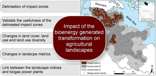
to delineate the zones of different level of impacts in terms of landscape change by biogas production in agrarian landscapes based on a density map of installed electrical capacity (IC) of the biogas power plants;
(2)
to quantify the impact of biogas power plants via size- and shape- related landscape metrics as well as diversity indices and to investigate the statistical relationships between the IC of biogas power plants and the various metrics.
The main outcome of our study is that we can delineate different impact zones of landscape change based on the installed electrical capacity density of biogas power plants for a federal state in northern Germany. These areas are highly affected by biogas production. We analysed the distribution and changes of land use categories and landscape indices inside of the impact zones to show the usefulness of this method.

2. Materials and Methods
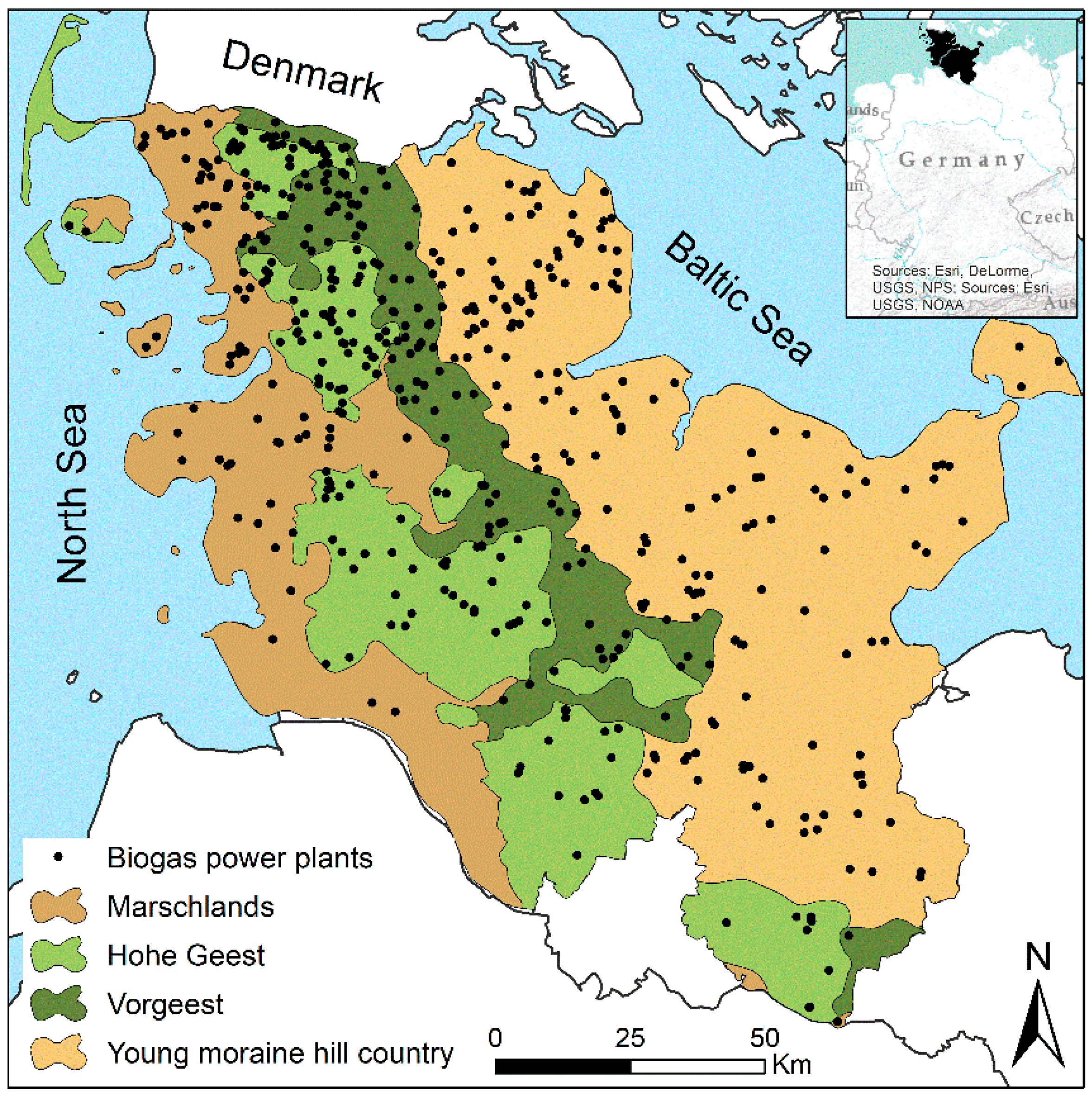
2.1. Study Area

Schleswig-Holstein, the northernmost Federal State of Germany, serves as the study area. It is surrounded by the Baltic Sea in the east, Denmark to the north and the North Sea to the west (Figure 1). The climate is humid with a mean annual temperature of 8.6 °C and mean annual precipitation of 878 mm (weather station Schleswig, 1981–2010, [43]). Schleswig-Holstein has a high level of agricultural use: in 2016, 41.5% of the federal-state’s area was arable land, 20.7% pasture, 10.6% forest, 13.2% sealed area and 14% other land cover types [44].
Based on the geological formations that developed during glacial and Holocene times, Schleswig-Holstein can be divided into four main landscapes from West to East: the “Marschlands”, the “Hohe Geest” representing the slightly elevated and eroded remains of terminal moraine tills of the penultimate glaciation (Saalian), the glacial outwash plain (“Vorgeest”), and the “Young moraine hill country” covering the eastern parts of Schleswig-Holstein. The Young Moraine Hill Country is characterized by glacial deposits of the Weichselian glaciation. Parent material for soil development mainly consists of sandy loamy to loamy textures, providing highly fertile soils, such as Luvisols, Cambisols and their stagnic subtypes (according to Food and Agriculture Organization of the United Nations (FAO) [45]). The Young Moraine Hill Country is intensively used for crop production, mainly winter wheat (Triticum aestivum L.), barley (Hordeum vulgare L.) and oilseed rape (Brassica napus L.). In contrast, the sandy deposits of the outwash plain (“Vorgeest” and “Hohe Geest”) are characterized by less fertile soils such as Podzols and podsolic Gleysols and frequently wetted Gleysols at deeper positions. While the latter are typically used as meadow and pastureland for livestock farming, the nutrient-poor and water-limited podzolic soils are traditionally cultivated with silage maize (Zea mays L.) and rye (Secale cereale L.) for livestock feeding. The Marshlands on the western part of Schleswig-Holstein have developed since the end of the last ice age. They consist mainly of fine-grained marine sediments with higher shares of silt and clay deposited by the North Sea during the Holocene sea level rise. The younger soils (Calceric Fluvisols/Gleysols) of the Marshlands are highly productive and dominantly used for winter wheat production. The older and frequently wet marshland soils provide less favourable conditions for arable farming and generally used only for pasture.

2.2. Data Sources and Databases

Small-scale land cover and land-use data for the study site were extracted from the Corine Land Cover (CLC) project data. This data was used to calculate the landscape metric and land cover diversity parameters (Table 1). The CLC data sets are based on satellite image raster data and represent land cover and land-use in Europe at a scale of 1:100,000 at different years. They include 44 classes of land cover and land use, of which 37 are relevant for Germany [46]. A 25 ha minimum mapping unit is used to represent areal unities while linear land cover units are represented with a minimum width of 100 m [34,44,47]. In this study, CLC data sets for the years 2000 and 2012 were used, because the first biogas power plants were constructed around 2000 and subsequently increased strongly in number until at least 2012.
Statistical data from the German Agricultural Structure Survey (Agrar-Struktur-Erhebung, ASE) was used to calculate land cover and crop diversity metrics on municipality and landscape level (see Table 1). This statistical survey is conducted as a full census that gathers data on farm structures and land use as well. For the study region, results from the years 2003 and 2010 were available aggregated at municipality (1106 municipality in Schleswig-Holstein) and at landscape level, provided by the statistical authority. For calculating diversity metrics, the hectares of land-use for crops and pasture were joined to official municipality geodata inside the study area [44].
Data on the location and installed electrical capacity (IC) of biogas power plants in Schleswig-Holstein were provided by the State Office for Agriculture Environment and Rural Spaces [48]. The dataset used in this study gives information on 925 sites of biogas power plants from the year 2014 (Figure 1), including the characteristics of the generators used to produce electricity from biogas.
We used these three different datasets from five different years as, they are not available for the same year.

2.3. Landscape Metrics

Landscape metric parameters are important quantitative implements in landscape ecology [51]. The selection of area and shape related landscape metrics used in this work (see below), is based on the work of Szabó [52] and Walz [51]. The software developed by Lang and Tiede [53] was employed for the calculation of landscape metrics. Concerning pattern analyses (e.g., [54,55,56,57]), this study uses parameters that are suited to indicate temporal changes in area, structure and diversity at the landscape and patch level (for more details see Table A1). Patch level metrics, created for individual land cover patches, characterize the spatial character and context of patches. These patch metrics serve primarily as the computational basis for developing a landscape metric. Class level metrics unify the patches of a given land cover type (class). Landscape level metrics are integrated over all patch types or classes over the full extent of the data. Like class metrics, they may be integrated by a simple or weighted averaging, or may reflect aggregate properties of the patch mosaic.
As many of the available measures of landscape metrics are partially or completely redundant, such as patch density (PD) and mean patch size (MPS), only the MPS was considered in this study. The MPS has been widely applied in landscape monitoring, since it is commonly agreed that the occurrence and abundance of different kinds of species and species richness as well, strongly correlates with the patch size. Amongst patch size metrics, edge-metrics can be used to characterize the spatial grain and the structural variety of a landscape [39]. The total edge (TE) of all patches in a selected landscape is known to have several effects on ecological phenomena [30]. Both of the landscape indicators, MPS and TE, were used to represent the continuity of the landscape’s structure during the observed period from 2000 to 2012. The Mean Shape Index (MSI) was calculated to further describe the changes in the geometrical complexity of a patches. The mean fractal dimension index (MFRACT) is a normalized shape index in which the perimeter and area are log transformed [39].
For evaluating changes in landscape and in structural richness, the Shannon diversity (SDI), evenness (SEI) and the richness indexes (RI) according to Uuemaa et al. [30] were applied, involving all land use classes in the study area.
To assess the effects of the increasing number of biogas power plants on the landscape patterns’ grain size, MPS and TE have been chosen. The effects on the shape complexity of the individual land use types were quantified by using MSI and MFRACT as indicators. We used the area weighted mean (AWM) values of these indices in the statistical calculations. AWM equals the sum of all patches in the area, of the corresponding patch type multiplied by the proportional abundance of the patch and divided by the sum of the patch areas.

2.4. Spatial and Statistical Analysis

In order to relate the changes in land cover and land cover pattern to the IC of biogas power plants inside an area we delineated three impact zones of different density of IC (MW km−2) using Kernel Density calculation within ArcGIS 10.3 software [58]. Separation of the single IC density classes followed the Jenks natural breaks classification method [59]. In detail, three impact zones were defined: “impact zone A” (1.03 to 2.46 MW km2), “impact zone B” (0.3 to 1.03 MW km2), and “impact zone C” (< 0.3 MW km2) (Figure 2).
The structural characteristics of land cover and the land cover pattern inside of these impact zones and their changes were analysed using the CLC data sets. AWM values have been calculated based on the class level landscape indices in the three impact zones and in the total study area using the Geospatial Modelling Environment [60]. This tool uses just the patches which having their centroids inside a given impact zone. Area-weighted metrics are more meaningful in ecology than the means as suggested by Gustafson [61]. Based on CLC data, the area-weighted size (AWMPS), edge (AWMTE) and shape metrics (AWMFRACT, AWMSI) were calculated for the landscape level and the class level (classes are patches of “arable land” and “pastures”) considering the individual impact zones and the entire federal-state of Schleswig-Holstein. CLC data sets were also used to calculate the landscape level diversity indices (SDI, SEI and RI) for the three impact zones of the study area. The same indices have been calculated for the municipality level using the ASE data set to detect changes in agricultural diversity (all kinds of agricultural land use) and crop diversity (only crop types) at local scale.
The landscape metrics related to size and shape (AWMPS, AWMTE, AWMFRACT) were calculated using the V-Late 2.0 (Vector-based Landscape analysis tool extension of ArcGIS 10.2) tool [53]. The same applies for the land cover diversity indices (SDI, SEI, RI) derived from CLC data. For calculating the same agricultural diversity indices from the ASE data-set, a Microsoft Excel add-in [62] has been applied. We calculated the area weighted shape and size related landscape indices, and the averages of the land cover and crop diversity indices for each municipality of the study area. We counted and summarized every biogas power plants and their IC (MW) in every municipality. At the statistical analysis part of the work, we selected the municipalities (containing the metrics and IC values) inside every impact zone and calculated the coefficient value for every impact zone. We ran a one-way analysis of variance (ANOVA) test on our municipality dataset (containing the landscape metrics and diversity indices). This analysis can be performed on a dataset with three or more groups, so the three impact zones were declared as groups. The ANOVA test is a technique to compare the means of groups using F distribution. The null hypothesis is that samples in all groups are drawn with the same mean values. We used the Tukey post hoc multiple comparison, which shows, which groups differed from each other. For statistical analyses between the IC of biogas power plants, and the landscape indices describing the shape and size characteristics of land cover patches, and the land cover diversity, the non-parametric Spearman rank correlation was used. IBM SPSS Statistics 22 software [63] was used for statistical evaluation.

3. Results

3.1. Delineation of the Bioenergy Impact Zones

Kernel density calculation enabled the separation of three impact zones of different density of IC of biogas power plants (Figure 2). We named the three delineated impact zones based on the density of biogas power plants’ installed electrical capacity: impact zone A = 1.03–2.46 MW/km2, impact zone B = 0.3–1.03 MW/km2, impact zone C = 0–0.3 MW/km2. Impact zone A is mainly located in the central northern part of Schleswig-Holstein, which is traditionally used for livestock- breeding and milk production. Areas of impact zone B comprise nearly all the interior landscapes, while impact zone C areas occur along the periphery of the federal state.

3.2. Validation of the Delineated Impact Zones

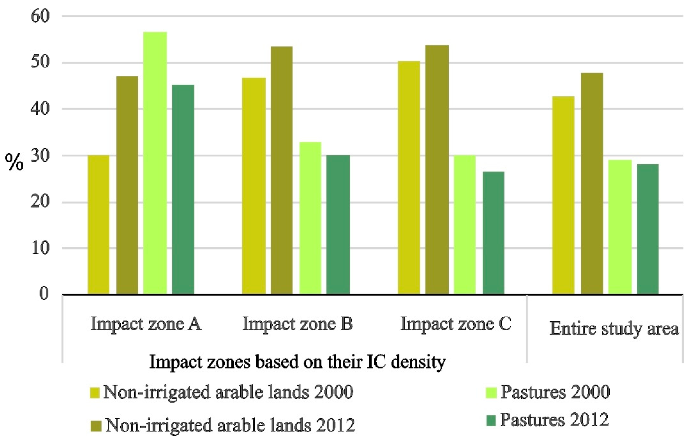
3.2.1. Land Cover Changes Inside the Impact Zones

Based on the CLC data sets from 2002 and 2012 various changes regarding land use can be detected, in the entire study area. The biggest changes relate to the CLC class “non-irrigated arable land” and “pastures” inside the delineated impact zones. According to Bossard et al. [47], the land use class "non-irrigated arable land" refers to land parcels cultivated with annually harvested non-permanent crops, usually grown in a crop rotation. The land use class “pasture” subsumes all permanent grassland characterized by agricultural use, like grazing or harvesting of grass. Regarding the entire study area, the amount of arable land increased by 5%, while the pasture decreased by 1%. Between 2000 and 2012, impact zone A reveals an increase of "non-irrigated arable land” by 17% and a decrease in pasture area by 11%. Inside impact zones B and C, only small changes of a few percent were registered (Figure A1).
Based on the ASE dataset, we analysed the changes in different agricultural land use types for the entire study area. Figure 3 shows the changes in silage maize and pastures area. These land use types experienced the greatest change from 2003 to 2010 (Figure 3). The Pasture area decreased by 68,000 hectares, while the silage maize acreage increased by 89,000 hectares.
Correlating the ASE data to the impact zones shows that the proportion of silage maize area strongly increased, mainly inside impact zone A. In some municipalities, the proportion of silage maize amounts to 66% of the total area of agricultural land use (Figure 4).
Compared to the entire state of Schleswig-Holstein, where the silage maize acreage increased on average 9% between 2003 and 2010, impact zone A shows a stronger positive change in silage maize acreage of about 20%. During the same period, the pasture area decreased by the same percentage. The biggest changes in land use appear in the northern parts of the glacial outwash plain (Vorgeest). In contrast, only modest changes occurred in the impact zones C (comparing Figure 4a,b). Furthermore, the ASE data indicate that a large proportion of pasture had been transformed into arable land for silage maize production (Figure A2).

3.2.2. Landscape Metrics Inside the Impact Zones

The effects of increased biogas production on the spatial structures of “non-irrigated arable land” and “pasture” were quantified via a set of area, edge and shape related landscape metrics calculated from CLC data. In general, Figure A3 reveals decreases in size (AWMPS), perimeter (AWMTE) and complexity (AWMSI, AWMFRACT) for the arable land and pastures compared to state wide conditions. Further, the data for impact zone A deviate noticeably from the others. Here, the edge length indicator AWMTE and the complexity indicators AWMSI and AWMFRACT of arable land increased from 2000 to 2012. In contrast, the same indicators for pasture areas show a strong decrease. The patch sizes (AWMPS) of pastures also declined drastically during this period. These findings suggest that patches occupied by cropland became bigger and more complex, while the perimeters of these patches increased relative to area they enclose. For pastureland the opposite trend occurred, as patches became smaller and more compact. Except for the AWMFRACT, which shows an increase for arable land and pastures in the impact zone B and C, all other shape and size related patch level metrics reveal declining values.

3.2.3. Land Cover Diversity Inside the Impact Zones

Land cover diversity indices (RI, SDI and SEI) were calculated from CLC data. They show a decreasing tendency between 2000 and 2012 inside the entire study area. The strongest decline can be observed for the SDI which decreased from 1.207 to 1.067. Furthermore, the SEI changed from 0.403 to 0.356 (Table A2). Impact zone A is characterized by the smallest SDI and SEI numbers, while the RI does not reflect any changes in these areas.
Moreover, ASE statistics indicate a strong decline in agricultural and crop diversity. The richness index (RI) calculated for agricultural diversity decreased in the individual impact zones as well as in the entire area of the federal state of Schleswig-Holstein (Table 2). Strongest reductions of RI occurred in areas of impact zone A, which also revealed the largest negative changes in SDI, while the SEI only varied slightly (Table 2).
For crop diversity areas of impact zone A show the strongest change, compared to the entire study area as well as to the impact zones B and C.

3.2.4. Link between Installed Electrical Capacity (IC) and Changes in Land Use and Landscape Indices in the Impact Zones

There was a statistically significant difference between groups as determined by one-way ANOVA test, non-irrigated arable land: AWMPS (F (2, 1087) = 27, p = 3.57−12), AWMTE (F (2, 1087) = 25.6, p = 1.35−11), AWMSI (F (2, 1087) = 10.89, p = 2.07−5), AWMFRACT (F (2, 1087) = 0.15, p = 0.6) (Table A3 and Table A4); pastures land: AWMPS (F (2, 1087) = 5.94, p = 0.003), AWMTE (F (2, 1087) = 5.66, p = 0.004), AWMSI (F (2, 1087) = 5.42, p = 0.005), AWMFRACT (F (2, 1087) = 4.71, p = 0.009) (Table A5 and Table A6). According to these results of the ANOVA test, the three delineated impact zone show significant difference in the mean of the landscape indices. The non-irrigated arable land patches’ shape and size characteristics show a significant positive correlation (p < 0.05) with the IC of each impact zones and the entire area of Schleswig-Holstein, while the same landscape indices for the pasture land cover patches are negatively (but not significantly) correlated with IC. We used just the municipality dataset with IC and ASE data for this calculation.
The tightest positive significant correlations (p < 0.01) between IC and AWMPS, AWMTE and AWMSI were measured in case of the “non-irrigated arable land use” patches located inside the impact zone A, while AWMFRACT only shows a weaker, but still significant correlation. Significant positive correlation coefficients were observed at the AWMSI of arable land, while negative coefficients were registered for AWMFRACT (r = −0.250, p < 0.05) related to pasture land (Table 3).
Inside impact zone C, only the AWMPS yields a significant correlation (r = 0.319, p < 0.05) for arable land use. Inside impact zone B, no significant correlation was found between IC and the single indices.
Based on the ASE dataset we found significant correlations between the different types of agricultural land use and the installed capacity of biogas power plants (Table 4). Silage maize acreage strongly positively correlates (r = 0.572, p < 0.01) with the IC density of the study area as well as with the individual impact zones (p < 0.01). Significant correlations were calculated for regions of highest biogas production, while correlations get weaker with a decrease in IC density.
There was a statistically significant difference between groups as determined by one-way ANOVA test, SDI (F (2, 1108) = 26.62, p = 5.09−12), SEI (F (2, 1108) = 14, p = 9.98−7), RI (F (2, 1108) = 20.63, p = 1.6−9) (see Table A7 and Table A8). Based on the ANOVA test the mean values of the diversity indices in the impact zones show significant differences. Finally, significant inverse correlations between the IC of the impact zones and land cover diversity (SDI, RI SEI) can be determined (Table 5). Impact zone A shows negative correlation coefficients with the diversity indices, SDI (r = −0,234, p < 0.01), SEI (r = −0.257, p < 0.01) and RI (r = −0.297, p < 0.01). Impact zone C does not correlate with the individual diversity indices. The findings in Table 5 suggest a decreasing influence of biogas production on landscape diversity with the decline of IC in a region.

4. Discussion

4.1. Comparative Analyses of the Bioenergy Impact Zones

The existing biogas power plants (419 MW installed electrical capacity) in 2014 according to Melund [64] are mostly concentrated in the central and north-western glacial outwash plain of Schleswig-Holstein (see Figure 1), where soils of relatively poor quality dominate and there is a relatively high livestock density. The intensive use of biogas power plants in this area is offering a profitable additional or alternative income to farmers, compared to other common local land-use practices like permanent pasture for dairy farming fodder production. In addition, biogas power plants provide opportunities to process manure, which is available in large amounts in regions of high cattle density [10,14,22,23,65].
In many cases, fields that were formerly farmed with a diverse crop rotation today possess higher shares of silage maize, especially when they are located in the vicinity of biogas power plants in order to reduce transportation distances and to optimize economic production chains for biomass use [10,13,24,66]. Nevertheless, whether one can directly link locally observed trends of decreasing grassland area and simultaneously increasing silage maize acreage, energy production from biogas is still under discussion. Lüker-Jans et al. [13] investigated the relation between the expansion of silage maize area, conversion of pasture to arable land and the distance to existing biogas power plants for the Federal State of Hesse in Central Germany, using statistical and farm specific data sets aggregated on municipality level. They found a significant correlation between existing and additional maize area and the distance to biogas power plants and a relationship between the vicinity of biogas power plants and conversion of pasture but also high correlation between existing maize area and livestock density. The proportion of silage maize increased in the entire study area from the beginning of 2000s (Figure A2), and based on the Figure 3 it increased by around 90,000 ha, while the pastures had a decrease around 70,000 ha. Figure 4 shows the municipalities where the increase was the highest and the silage maize maximum proportion reached the 66%. The expansion of the silage maize was most dynamic in the impact zone A. One can say that silage maize is probably the most significant indicator of the bioenergy generated transformation of the agricultural landscape.
The area of silage maize reveals a positive correlation (r = 0.572; p < 0.01) with the IC of biogas power plants and the strongest correlation compared to all other types of agricultural land use and arable crops (Table 4). The decrease in pasture area coincides with the start of increased silage maize growing. According to the ASE data set other crop and land use types did not increase to that proportion as silage maize did. For a small catchment in Germany Kandziora et al. [28] could prove the same results that the pasture area decreased to 50% from 1987 to 2007. The statistical analysis in our study make obvious that the silage maize acreage as well as the area of arable land (r = 0.541) and pasture (r = 0.457) significantly correlate (p < 0.01) with the density of IC (Table 4). Silage maize is the most common crop used for feeding the fermentation tanks. Interestingly, we found that the pasture area also positively correlates with IC. One reason might be that the farmers use the sown grass as a substrate for biogas production. According to Auburger et al. [67], the harvesting of pastures for biogas power plants could be an alternative way to replace silage maize to a limited degree, however this process is more expensive, so that farmers usually prefer the use of silage maize and manure for biogas production.

4.2. Statistical Analysis of the Landscape Metric Parameters in the Bioenergy Impact Zones

Comparing the two CLC data sets from 2000 and 2012 reveals that the patches of arable lands became larger and complex, while the patches covered with pasture became more compact, including a reduced length of their margins/edges. This holds especially true for those regions that have a high density of installed biogas power plants. These findings indicate that a higher percentage of arable fields become interconnected, grow in size and become more complex in shape, while a lesser number of isolated patches of pasture remains (Figure A3). These results fit to the work of Leuschner et al. [65], who showed for Schleswig-Holstein that from 1950 on the arable lands - and in the last decade the silage maize fields - were getting bigger with a more complex shape, while pastures were getting smaller, more fragmented and isolated.
As shown for the arable land located in the impact zone A, the AWMSI needs to be carefully interpreted and not decoupled from other indices, such as the AWMPS or AWMTE. A higher degree of compactness is not necessarily equivalent to a decrease in patch size or a reduction of edge lengths. The situation mainly depends on the shape of the patches. In arable land patches with noticeable increases in AWMTE and also in complexity as indicated by AWMFRACT (Figure A3), the degree of compactness can also increase, for example, when the field plots are expanded to all sides and have more or less equal widths and length ratios.
The significant positive correlation between the IC and the area of arable land in impact zone A occurs because of the higher demand for silage maize, which is associated with increases in patch size and complexity within the landscape. In contrast, all landscape metrics indicators calculated for the pasture land use type reveal a significant inverse correlation with biogas production intensity. In the case of arable land, the AWMSI shows highest correlation with the IC density of biogas power plants, suggesting that an increase in IC, mainly affects the shape and complexity of the cropland patches. From the indices derived for pasture land, the MFRACT is most strongly correlated to IC inside the impact zone A, implying that the intensity of biogas production contributes mainly to the form of patches, coupled with a higher fractioning of grassland patches, as indicated by the negative significant correlation between AWMSI and IC density. In the impact zone A the AWMSI and AWMFRACT could be an indicator of the bioenergy generated transformation of agricultural landscapes, and they could help identify of this transformation. Uuemaa et al. [31] found that these are the most relevant metrics to describe landscape complexity and fragmentation, also for effect on species diversity.

4.3. Land Cover Diversity Changes in the Bioenergy Impact Zones

Land cover diversity indices were calculated from the CLC and ASE datasets, and we used the three most common diversity indices [68]. Regarding changes in landscapes and agricultural diversity, the RI index negatively and significantly correlated to the intensity of biogas production, and compared to all other diversity indices it has the highest negative correlation coefficient. The correlation between the RI and the IC density of biogas power plants is significant (r = −0.297, p < 0.01, Table 5), suggesting the RI to be a suited indicator to identify the bioenergy generated transformation in agricultural used areas [13,16].
Calculation based on CLC data shows the smallest values for SDI in the impact zone A and the strongest decrease of RI compared to the other regions (Table 5). The same correlation holds true for SDI, indicating an increase in unevenness related of the different land use classes and crop types, as arable land is increasingly used for silage maize growing at a higher area percentage, including a higher share of maize monoculture. These support the knowledge from regional studies concerning the recent development in “energy landscapes” of Schleswig-Holstein, stating biogas production as the main driver of the landscape and land use change (e.g., [19,69]).
A decreasing trend in agricultural land cover diversity can be demonstrated by comparing the ASE data from 2003 and 2010, where most of the biogas power plants were newly constructed. As already described for the CLC data set, the strongest decline in SDI and SEI numbers goes along with the increase in IC density, where the smallest numbers of these indicators are typical for those regions with the highest densities of biogas generated electricity (Table A2). Regarding the arable land, however, there is a strong increase in the proportion of silage maize, while other agricultural land use types changed by a few percent. Considering crop diversity, a negative change of SDI, SEI and RI can be observed for all impact zones, with the strongest decline occurring in the impact zone A (Table 2). This indicates that the increase in silage maize production subsequently replaces other crops originally grown in these landscapes to a higher degree, which contributes to a loss of crop diversity and a depletion of landscape diversity. These results fit to the work of Jerrentrup et al. [70].
In order to prevent the undesired effects of land cover pattern change and landscape diversity decrease caused by the bioenergy-generated transformation of agricultural landscapes, landscape metrics and diversity indicators generated from data of various spatial scales can support a well-informed approach to landscape management. As shown in this study, spatial landscape metrics and diversity indicators are suited to spatially detect changes in land cover and crop diversity and in the landscape’s structure. In this example, landscape metrics have demonstrated that an uncontrolled bioenergy-generated transformation (expansion of maize cropping) may negatively affect landscape diversity.

5. Conclusions

This study shows that changes in land use, land cover pattern and landscape diversity caused by a bioenergy-driven transformation of agricultural landscapes can be identified via landscape metrics and diversity indicators applied to readily available data with different degrees of spatial and thematic aggregations. It reveals that the fostered production of electrical energy by biogas power plants can negatively affect the sizes and shapes of former pasture lands and increases the area, size and complexity of arable land patches. Moreover, for the study area in Northern Germany, the application of a Kernel density analysis based on data on the installed electrical capacity (IC) of biogas power plants could spatially identify the main impact zones (hot spots) of biogas energy generated declining land cover and crop diversity. Furthermore, this study provides quantified data on the spatio-temporal changes in landscape metrics indicators related to the different intensity zones of bioenergy generated landscape transformation. According to our findings, the Kernel density map of the electrical capacity of biogas power plants are representing the impact zones of the biogas energy introduction. The calculations based on the Corine Land Cover database can be replicated in the countries of the European Union, where the CLC database exist, but other land cover or land use dataset can be adapting. The GIS tools used, released under general public licence (GPL), therefore are free to use for anyone, with the exception of Environmental Systems Research Institute (ESRI) ArcGIS, which is proprietary. The quality of calculated outcomes could be improved with the availability of remote sensing data of higher spatial and spectral resolution, and of a higher recovery rate, enabling a more detailed classification of land use and crop type, as shown by, for example, Kuhwald et al. [71].

Author Contributions

Conceptualization, N.C., M.S., M.K., P.S. and R.D.; Formal analysis, N.C.; Methodology, N.C., P.S.; Resources, M.S.; Supervision, P.S. and R.D.; Visualization, N.C. and M.S.; Writing—original draft, N.C. and M.S.; Writing—review & editing, M.K., P.S. and R.D.

Funding

The Deutsche Bundesstiftung Umwelt MOE Scholarship Program founded N.C. We acknowledge financial support by Land Schleswig-Holstein within the funding programme Open Access Publikationsfonds.

Acknowledgments

We express our sincere thanks to James Petersen (Texas State University) for lingual editing an early draft and to Kilian Etter (Kiel University) for lingual editing the manuscript. We thank the anonymous referees for their valuable recommendations and suggestions.

Conflicts of Interest

The authors declare no conflict of interest.

Appendix

Figure A1. Proportion of the non-irrigated arable lands and pastures at utilized land area in the entire study area and in the Installed electrical Capacity (IC) density-based impact zones, based on CLC 2000 and 2012 database.
Sustainability 11 02500 g0a1
Figure A2. Percentage of pasture and silage maize areas in the entire study area and in the Installed electrical Capacity (IC) density-based impact zones, based on ASE 2003 and 2010 database.
Sustainability 11 02500 g0a2
Figure A3. Size and shape related class level landscape metrics of non-irrigated arable lands and pastures, based on CLC 2000 and CLC 2012 databases (IC = Installed electrical Capacity, AWMPS = Area weighted mean patch size, AWMTE = Area weighted mean total edge, AWMSI = Area weighted mean shape index, AWMFRACT = Area weighted mean fractal dimension index).
Sustainability 11 02500 g0a3
Table A1. Description of area, edge, shape and diversity metrics used in this study (based on [31,51,72,73,74,75,76,77]).
Investigated FeatureDatabase Used for CalculationIndexName and DescriptionCorresponding Question
AreaCLCMPSMean Patch Size
M P S = j = 1 n a i j n i
where aij represents the area of the jth patch in the ith class, ni represents the number of patches in the ith class, n represents the number of patches (>0)
What is the average land cover patch size, and how are the values distributed?
EdgesCLCTETotal Edge
T E = k = 1 m e i k
where eik represents the edge length between the ith and kth patch types, m represents the number of the patch class (<=0).
How much of a landscape or a land cover patch type is composed of edges?
Shape complexityCLMSIMean Shape Index
M S I = j = 1 n ( p i j π * a i j 2 ) n i
where pij represents the perimeter of the jth patch in class ith, aij represents the area of the jth patch in class ith, ni represents the number of patches in the ith class, n represents the number of patches (>=1)
How compact are the patches on average (in comparison to a circle)?
CLCMFRACTMean Fractal Dimension
M F R A C T = j = 1 n ( 2 ln p i j ln a i j ) n i
where pij represents the perimeter of the jth patch in class ith, aij represents the area of the jth patch in class ith, ni represents the number of patches in the ith class, n represents the number of patches (1–2)
How complex or irregular is the form of the land cover patch?
Diversity metricsCLC and ASESDIShannon Diversity Index
S D I = i m ( P i * ln ( P i ) )
Where (m) represents the number of different land cover types, Pi = the relative abundance of different land cover types
How diverse is the landscape?
CLC and ASESEIShannon Evenness Index
S E I = i m ( P i * ln ( P i ) ) ln ( m )
SEI covers the number of different land cover types (m) and their relative abundance (Pi)
How equal is the distribution of the land cover patches in the landscape?
CLC and ASERIRichness Index
presents simply the variety or number of patch types in landscape level.
How many different land cover patch types build the landscape?
Table A2. Land cover diversity indices between 2000 and 2012, based on CLC database (IC = Installed electrical Capacity).
YearLandscape Diversity IndicesImpact Zones Based on Their IC Density Total Study Area
Impact Zone AImpact Zone BImpact Zone C
2000Richness20323232
Shannon Diversity1.2071.5061.5231.757
Shannon Evenness0.4030.4350.440.507
2012Richness20313133
Shannon Diversity1.0671.3541.4641.597
Shannon Evenness0.3560.3940.4190.457
Table A3. One-way ANOVA of landscape indices of non-irrigated arable lands in the three impact zone.
Sum of SquaresdfMean SquareFSig.
AWMPSBetween Groups2.26 × 101921.13 × 1019273.578 × 10−12
Within Groups4.54 × 102010874.18 × 1017
Total4.77 × 10201089
AWMTEBetween Groups1.11 × 101425.56 × 101325.6121.352 × 10−11
Within Groups2.36 × 101510872.17 × 1012
Total2.47 × 10151089
AWMSIBetween Groups1.62 × 1032811.28910.8912.074 × 10−5
Within Groups8.10 × 104108774.491
Total8.26 × 1041089
AWMFRACTBetween Groups2.56 × 10−320.0010.5150.598
Within Groups2.68110780.002
Total2.6841080
Table A4. Tukey post hoc test of landscape indices of non-irrigated arable lands in the three impact zone.
Dependent VariableMean Difference (I-J)Std. ErrorSig.
AWMPSImpact zone AImpact zone B −1.665 × 1085.84 × 1071.226 × 10−2
Impact zone C −4.047 × 1086.08 × 1075.223 × 10−9
Impact zone BImpact zone A 1.665 × 1085.84 × 1071.226 × 10−2
Impact zone C −2.382 × 1084.29 × 1071.103 × 10−7
Impact zone C Impact zone A 4.047 × 1086.08 × 1075.223 × 10−9
Impact zone B 2.382 × 1084.29 × 1071.103 × 10−7
AWMTEImpact zone A Impact zone B −3.833 × 1051.33 × 1051.123 × 10−2
Impact zone C −9.048 × 1051.38 × 1055.384 × 10−9
Impact zone B Impact zone A 3.833 × 1051.33 × 105 1.123 × 10⁻²
Impact zone C −5.215 × 1059.78 × 1043.550 × 10−7
Impact zone C Impact zone A 9.048 × 1051.38 × 1055.384 × 10−9
Impact zone B 5.215 × 1059.78 × 1043.550 × 10−7
AWMSIImpact zone A Impact zone B −1.0297.79 × 10−10.384
Impact zone C −3.2318.11 × 10−12.140 × 10⁻⁴
Impact zone B Impact zone A 1.0297.79 × 10−10.384
Impact zone C −2.2035.73 × 10−13.737 × 10⁻⁴
Impact zone C Impact zone A 3.2318.11 × 10−12.140 × 10⁻⁴
Impact zone B 2.2035.73 × 10−13.737 × 10⁻⁴
AWMFRACTImpact zone A Impact zone B 0.0044.51 × 10−30.590
Impact zone C 0.0044.69 × 10−30.637
Impact zone B Impact zone A −0.0044.51 × 10−30.590
Impact zone C 0.0003.32 × 10−30.998
Impact zone C Impact zone A −0.0044.69 × 10−30.637
Impact zone B 0.0003.32 × 10−30.998
Table A5. One-way ANOVA of landscape indices of pastures in the three impact zone.
Sum of SquaresdfMean SquareFSig.
AWMPSBetween Groups1.18 × 101825.91 × 10175.9410.003
Within Groups1.08 × 102010889.95 × 1016
Total1.09 × 10201090
AWMTEBetween Groups1.08 × 101325.41 × 10125.6580.004
Within Groups1.04 × 101510889.56 × 1011
Total1.05 × 10151090
AWMSIBetween Groups742.3872371.1945.4250.005
Within Groups74,438.765108868.418
Total75,181.1531090
AWMFRACTBetween Groups0.02720.0144.7140.009
Within Groups3.14210880.003
Total3.1691090
Table A6. Tukey post hoc test of landscape indices of pastures in the three impact zone.
Dependent VariableMean Difference (I-J)Std. ErrorSig.
AWMPSImpact zone A Impact zone B −6.27 × 1072.84 × 1070.071
Impact zone C 4.37 × 1062.96 × 1070.988
Impact zone B Impact zone A 6.27 × 1072.84 × 1070.071
Impact zone C 6.71 × 1072.09 × 1070.004
Impact zone C Impact zone A −4.37 × 1062.96 × 1070.988
Impact zone B −6.71 × 1072.09 × 1070.004
AWMTEImpact zone A Impact zone B −1.52 × 1058.81 × 1040.196
Impact zone C 6.08 × 1049.17 × 1040.785
Impact zone B Impact zone A 1.52 × 1058.81 × 1040.196
Impact zone C 2.13 × 1056.49 × 1040.003
Impact zone C Impact zone A −6.08 × 1049.17 × 1040.785
Impact zone B −2.13 × 1056.49 × 1040.003
AWMSIImpact zone A Impact zone B −7.17 × 10−27.45 × 10−10.995
Impact zone C 1.667.75 × 10−10.082
Impact zone B Impact zone A 7.17 × 10−27.45 × 10−10.995
Impact zone C 1.735.49 × 10−10.005
Impact zone C Impact zone A −1.67.75 × 10−10.082
Impact zone B −1.735.49 × 10−10.005
AWMFRACTImpact zone A Impact zone B 3.05 × 10−34.84 × 10−30.803
Impact zone C 1.25 × 10−25.04 × 10−30.035
Impact zone B Impact zone A −3.05 × 10−34.84 × 10−30.803
Impact zone C 9.48 × 10−33.56 × 10−30.022
Impact zone C Impact zone A −1.25 × 10−25.04 × 10−30.035
Impact zone B −9.48 × 10−33.56 × 10−30.022
Table A7. One-way ANOVA of diversity indices in the three impact zone.
Sum of SquaresdfMean SquareFSig.
SDIBetween Groups8.77624.38826.6235.09 × 10−12
Within Groups182.61411080.165
Total191.3901110
SEIBetween Groups3.54521.77313.9919.98 × 10−7
Within Groups140.38311080.127
Total143.9291110
RIBetween Groups76.733238.36620.6311.60 × 10−9
Within Groups2060.52211081.860
Total2137.2551110
Table A8. Tukey post hoc test of diversity indices in the three impact zone.
Dependent VariableMean Difference (I-J)Std. ErrorSig.
SDIImpact zone A Impact zone B −0.1500400.0365190.000126
Impact zone C −0.2680.0378690.000000
Impact zone B Impact zone A 0.1500.0365190.000126
Impact zone C −0.1180.0265990.000029
Impact zone C Impact zone A 0.2680.0378690.000000
Impact zone B 0.1180.0265990.000029
SEIImpact zone A Impact zone B −0.1220.0320190.000445
Impact zone C −0.1760.0332030.000000
Impact zone B Impact zone A 0.1220.0320190.000445
Impact zone C −0.0540.0233210.055313
Impact zone C Impact zone A 0.1760.0332030.000000
Impact zone B 0.0540.0233210.055313
RIImpact zone A Impact zone B −0.3600.1230.009628
Impact zone C −0.7630.1270.000000
Impact zone B Impact zone A 0.3600.1230.009628
Impact zone C −0.4030.0890.000021
Impact zone C Impact zone A 0.7630.1270.000000
Impact zone B 0.4030.0890.000021

References and Notes

  1. EU Directive 2009/28/EC of the European parliament and of the council of 23 April 2009 on the promotion of the use of energy from renewable sources and amending and subsequently repealing Directives 2001/77/EC and 2003/30/EC. Off. J. Eur. Union 2009, 52, 16–62.
  2. EEA Renewable Energy in Europe 2017. Recent Growth and Knock-on Effects. EEA Report No 3/2017. Available online: https://www.eea.europa.eu/publications/renewable-energy-in-europe-2017 (accessed on 27 April 2019).
  3. EC (European Commission) Optimal Use of Biogas from Waste Streams. An Assessment of the Potential of Biogas from Digestion in the EU beyond 2020—European Commission. Available online: https://ec.europa.eu/energy/en/studies/optimal-use-biogas-waste-streams-assessment-potential-biogas-digestion-eu-beyond-2020 (accessed on 9 May 2018).
  4. Sahoo, K.; Mani, S.; Das, L.; Bettinger, P. GIS-based assessment of sustainable crop residues for optimal siting of biogas plants. Biomass Bioenergy 2018, 110, 63–74. [Google Scholar] [CrossRef]
  5. Van der Horst, D.; Martinat, S.; Navratil, J.; Dvorak, P.; Chmielova, P. What can the location of biogas plants tell us about agricultural change? A Case Study from the Czech Republic. Deturope 2018, 10, 33–52. [Google Scholar]
  6. Di Leo, S.; Salvia, M. Local strategies and action plans towards resource efficiency in South East Europe. Renew. Sustain. Energy Rev. 2017, 68, 286–305. [Google Scholar] [CrossRef]
  7. Gao, M.; Wang, D.; Wang, H.; Wang, X.; Feng, Y. Biogas potential, utilization and countermeasures in agricultural provinces: A case study of biogas development in Henan Province, China. Renew. Sustain. Energy Rev. 2019, 99, 191–200. [Google Scholar] [CrossRef]
  8. Scheftelowitz, M.; Becker, R.; Thrän, D. Improved power provision from biomass: A retrospective on the impacts of German energy policy. Biomass Bioenergy 2018, 111, 1–12. [Google Scholar] [CrossRef]
  9. AdV Working Committee of the Surveying Authorities of the States of the Federal Republic of Germany—AdV-Online. Available online: http://www.adv-online.de/Products/Geotopography/ATKIS/ (accessed on 9 May 2018).
  10. Delzeit, R.; Britz, W.; Holm-Müller, K. Modelling regional input markets with numerous processing plants: The case of green maize for biogas production in Germany. Environ. Model. Softw. 2012, 32, 74–84. [Google Scholar] [CrossRef]
  11. Gasso, V.; Oudshoorn, F.W.; de Olde, E.; Sørensen, C.A.G. Generic sustainability assessment themes and the role of context: The case of Danish maize for German biogas. Ecol. Indic. 2015, 49, 143–153. [Google Scholar] [CrossRef]
  12. Appel, F.; Ostermeyer-Wiethaup, A.; Balmann, A. Effects of the German Renewable Energy Act on structural change in agriculture—The case of biogas. Util. Policy 2016, 41, 172–182. [Google Scholar] [CrossRef]
  13. Lüker-Jans, N.; Simmering, D.; Otte, A. The impact of biogas plants on regional dynamics of permanent grassland and maize area—The example of Hesse, Germany (2005–2010). Agric. Ecosyst. Environ. 2017, 241, 24–38. [Google Scholar] [CrossRef]
  14. Laggner, B.; Orthen, N.; Osterburg, B.; Röder, N. Ist die zunehmende Biogasproduktion die alleinige Ursache für den Grünlandschwund in Deutschland?—Eine Analyse von georeferenzierten Daten zur Landnutzung. Raumforsch. Raumordn. 2014, 72, 195–209. [Google Scholar] [CrossRef]
  15. Schleupner, C.; Link, P.M. Potential impacts on important bird habitats in Eiderstedt (Schleswig-Holstein) caused by agricultural land use changes. Appl. Geogr. 2008, 28, 237–247. [Google Scholar] [CrossRef]
  16. Brandt, K.; Glemnitz, M. Assessing the regional impacts of increased energy maize cultivation on farmland birds. Environ. Monit. Assess. 2014, 186, 679–697. [Google Scholar] [CrossRef] [PubMed]
  17. Lupp, G.; Steinhäußer, R.; Starick, A.; Gies, M.; Bastian, O.; Albrecht, J. Forcing Germany’s renewable energy targets by increased energy crop production: A challenge for regulation to secure sustainable land use practices. Land Use Policy 2014, 36, 296–306. [Google Scholar] [CrossRef]
  18. Link, P.M.; Schleupner, C. Agricultural land use changes in Eiderstedt: Historic developments and future plans. Coastline Rep. 2007, 9, 928–2734. [Google Scholar]
  19. Duttmann, R.; Hassenpflug, W.; Bach, M.; Lungershausen, U.; Frank, J. Winderosion in Schleswig-Holstein; Landesamt für Landwirtschaft, Umwelt und ländliche Räume des Landes Schleswig-Holstein (LLUR): Hamburg, Germany, 2011; ISBN 978-3-937937-56-4. [Google Scholar]
  20. Duttmann, R.; Schwanebeck, M.; Nolde, M.; Horn, R. Predicting Soil Compaction Risks Related to Field Traffic during Silage Maize Harvest. Soil Sci. Soc. Am. J. 2014, 78, 408. [Google Scholar] [CrossRef]
  21. Svoboda, N.; Taube, F.; Kluß, C.; Wienforth, B.; Kage, H.; Ohl, S.; Hartung, E.; Herrmann, A. Crop production for biogas and water protection—A trade-off? Agric. Ecosyst. Environ. 2013, 177, 36–47. [Google Scholar] [CrossRef]
  22. Klu. Biogaserzeugung und-nutzung: Ökologische Leitplanken für die Zukunft Vorschläge der Kommission Landwirt-schaft beim Umweltbundesamt (KLU); Agriculture Commission at the German Federal Environment Agency: Dessau-Roßlau, Germany, 2013. [Google Scholar]
  23. Claus, S.; Taube, F.; Wienforth, B.; Svoboda, N.; Sieleing, K.; Kage, H.; Senbayram, M.; Dittert, K.; Gericke, D.; Pacholski, A.; et al. Life-cycle assessment of biogas production under the environmental conditions of northern Germany: Greenhouse gas balance. J. Agric. Sci. 2014, 152, 172–181. [Google Scholar] [CrossRef]
  24. Duttmann, R.; Brunotte, J.; Bach, M. Spatial analyses of field traffic intensity and modeling of changes in wheel load and ground contact pressure in individual fields during a silage maize harvest. Soil Tillage Res. 2013, 126, 100–111. [Google Scholar] [CrossRef]
  25. Pantaleo, A.; De Gennaro, B.; Shah, N. Assessment of optimal size of anaerobic co-digestion plants: An application to cattle farms in the province of Bari (Italy). Renew. Sustain. Energy Rev. 2013, 20, 57–70. [Google Scholar] [CrossRef]
  26. Schmidt, C. Entwicklung der Anbauflächen für Silomais Seit 1999. Available online: https://tu-dresden.de/bu/architektur/ila/lp/ressourcen/dateien/Forschung/abgeschlossene-forschung/monitoring-kula-kartenserie-arbeitspaket2/karte5?lang=de (accessed on 11 March 2019).
  27. Oppelt, N.; Rathjens, H.; Kuhwald, K.; Oppelt, N.; Rathjens, H.; Doernhoefer, K. Integration of Land Cover Data into the Open Source Model SWAT. In Proceedings of the First Sentinel-2 Preparatory Symposium, Frascati, Italy, 23–27 April 2012. [Google Scholar]
  28. Kandziora, M.; Dörnhöfer, K.; Oppelt, N.; Müller, F. Detecting Land Use and Land Cover Changes in Northern German Agricultural Landscapes to Assess Ecosystem Service Dynamics. Landsc. Online 2014, 35, 1–24. Available online: https://www.landscapeonline.de/103097lo201435 (accessed on 28 April 2019). [CrossRef]
  29. Feng, Y.; Liu, Y.; Tong, X. Spatiotemporal variation of landscape patterns and their spatial determinants in Shanghai, China. Ecol. Indic. 2018, 87, 22–32. [Google Scholar] [CrossRef]
  30. Uuemaa, E.; Antrop, M.; Roosaare, J.; Marja, R.; Mander, Ü. Landscape Metrics and Indices: An Overview of Their Use in Landscape Research. Living Rev. Landsc. Res. 2009, 3, 1–28. [Google Scholar] [CrossRef]
  31. Uuemaa, E.; Mander, Ü.; Marja, R. Trends in the use of landscape spatial metrics as landscape indicators: A review. Ecol. Indic. 2013, 28, 100–106. [Google Scholar] [CrossRef]
  32. Schindler, S.; von Wehrden, H.; Poirazidis, K.; Wrbka, T.; Kati, V. Multiscale performance of landscape metrics as indicators of species richness of plants, insects and vertebrates. Ecol. Indic. 2013, 31, 41–48. [Google Scholar] [CrossRef]
  33. Borges, F.; Glemnitz, M.; Schultz, A.; Stachow, U. Assessing the habitat suitability of agricultural landscapes for characteristic breeding bird guilds using landscape metrics. Environ. Monit. Assess. 2017, 189, 166. [Google Scholar] [CrossRef]
  34. Szilassi, P.; Bata, T.; Szabó, S.; Czúcz, B.; Molnár, Z.; Mezősi, G. The link between landscape pattern and vegetation naturalness on a regional scale. Ecol. Indic. 2017, 81, 252–259. [Google Scholar] [CrossRef]
  35. Šímová, P.; Gdulová, K. Landscape indices behavior: A review of scale effects. Appl. Geogr. 2012, 34, 385–394. [Google Scholar] [CrossRef]
  36. Lausch, A.; Blaschke, T.; Haase, D.; Herzog, F.; Syrbe, R.-U.; Tischendorf, L.; Walz, U. Understanding and quantifying landscape structure—A review on relevant process characteristics, data models and landscape metrics. Ecol. Modell. 2015, 295, 31–41. [Google Scholar] [CrossRef]
  37. Weissteiner, C.J.; García-Feced, C.; Paracchini, M.L. A new view on EU agricultural landscapes: Quantifying patchiness to assess farmland heterogeneity. Ecol. Indic. 2016, 61, 317–327. [Google Scholar] [CrossRef] [Green Version]
  38. Turner, M.G. Landscape Ecology: What Is the State of the Science? Annu. Rev. Ecol. Evol. Syst. 2005, 36, 319–344. [Google Scholar] [CrossRef]
  39. Turner, M.G. Landscape Ecology: The Effect of Pattern on Process. Annu. Rev. Ecol. Syst. 1989, 20, 171–197. [Google Scholar] [CrossRef]
  40. Frondoni, R.; Mollo, B.; Capotorti, G. A landscape analysis of land cover change in the Municipality of Rome (Italy): Spatio-temporal characteristics and ecological implications of land cover transitions from 1954 to 2001. Landsc. Urban Plan. 2011, 100, 117–128. [Google Scholar] [CrossRef]
  41. Liu, H.; Weng, Q. Landscape metrics for analysing urbanization-induced land use and land cover changes. Geocarto Int. 2013, 28, 582–593. [Google Scholar] [CrossRef]
  42. Singh, S.; Srivastava, P.; Szabo, S.; Petropoulos, G.; Gupta, M.; Islam, T. Landscape transform and spatial metrics for mapping spatio-temporal land cover dynamics using Earth Observation datasets. Geocarto Int. 2015, 32, 1–34. [Google Scholar] [CrossRef]
  43. DWD Weather of Schleswig 1981–2010. Available online: https://www.dwd.de/EN/weather/weather_climate_local/schleswigholstein_hamburg/schleswig/_node.html (accessed on 13 August 2018).
  44. Bundesamt für Kartographie und Geodäsie Digitales Basis-Landschaftsmodell (AAA-Modellierung) Basis-DLM (AAA). Available online: http://www.geodatenzentrum.de/docpdf/basis-dlm-aaa.pdf (accessed on 9 May 2018).
  45. Fao World reference base for soil resources 2014 International soil classification system for naming soils and creating legends for soil maps Update 2015 WORLD SOIL RESOURCES REPORTS.
  46. EEA and ETC-TE CLC Update CLC 2000 Project. Technical Guidelines. Final Version. Available online: http://land.copernicus.eu/user-corner/technical-library/techrep89.pdf (accessed on 9 May 2018).
  47. Bossard, M.; Feranec, J.; Otahel, J. CORINE Land Cover Technical Guide—Addendum 2000 Part I State-of-Play Production Methods of the CORINE land Cover Database; European Environment Agency: Copenhagen, Denmark, 2000. [Google Scholar]
  48. Landesamt für Landwirtschaft, Umwelt und ländliche Räume Schleswig-Holstein. Data set on biogas power plants in Schleswig-Holstein 2014.
  49. EEA. The Thematic Accuracy of CLC 2000. Assessment Using LUCAS (Land Use/cover Area Frame Statistical Survey); EEA: Coppenhagen, Denmark, 2006. [Google Scholar]
  50. Statistiches Amt für Hamburg und Schleswig-Holstein. Kartenatlas zur Landwirtschaftszählung; Statistiches Amt für Hamburg und Schleswig-Holstein: Hamburg, Germany, 2010. [Google Scholar]
  51. Walz, U. Landscape Structure, Landscape Metrics and Biodiversity. Living Rev. Landsc. Res. 2011, 5. [Google Scholar] [CrossRef] [Green Version]
  52. Szabó, S. Tájmetriai mérőszámok alkalmazási lehetőségeinek vizsgálata a tájanalízisben; University of Debrecen: Debrecen, Hungary, 2009. [Google Scholar]
  53. Lang, S.; Tiede, D. vLATE Extension for ArcGIS—Vektorbasiertes Tool zur quantitativen Landschaftsstrukturanalyse; ESRI Anwenderkonferenz: Innsbruck, Austria, 2003. [Google Scholar]
  54. Baldwin, D.J.B.; Weaver, K.; Schnekenburger, F.; Perera, A.H. Sensitivity of landscape pattern indices to input data characteristics on real landscapes: Implications for their use in natural disturbance emulation. Landsc. Ecol. 2004, 19, 255–271. [Google Scholar] [CrossRef]
  55. Buyantuyev, A.; Wu, J. Effects of thematic resolution on landscape pattern analysis. Landsc. Ecol. 2007, 22, 7–13. [Google Scholar] [CrossRef]
  56. Uuemaa, E.; Roosaare, J.; Mander, Ü. Scale dependence of landscape metrics and their indicatory value for nutrient and organic matter losses from catchments. Ecol. Indic. 2005, 5, 350–369. [Google Scholar] [CrossRef]
  57. Wu, J. Effects of changing scale on landscape pattern analysis: Scaling relations. Landsc. Ecol. 2004, 19, 125–138. [Google Scholar] [CrossRef]
  58. Environmental Systems Research Institute (ESRI) ArcGIS Desktop 10.3, Redland, USA, 2014.
  59. Jenks, G. The Data Model Concept in Statistical Mapping. In International Yearbook of Cartography; George Philip: London, UK, 1967. [Google Scholar]
  60. Beyer, H.L. Geospatial Modelling Environment. Available online: http://www.spatialecology.com/gme/gmedownload.htm (accessed on 28 April 2019).
  61. Gustafson, E.J. Minireview: Quantifying Landscape Spatial Pattern: What Is the State of the Art? Ecosystems 1998, 1, 143–156. [Google Scholar] [CrossRef]
  62. Statistical Service Centre (SSC) Microsoft Excel add-in diversity calculator, Reading University, 2010.
  63. IBM SPSS IBM SPSS Statistics for windows 2013.
  64. MELUND. Monitoring Energiewende und Klimaschutz Schleswig-Holstein. 2018. Available online: https://www.schleswig-holstein.de/DE/Schwerpunkte/Energiewende/Daten/_documents/monitoring.html (accessed on 27 April 2019).
  65. Leuschner, C.; Krause, B.; Meyer, S.; Bartels, M. Structural change in the arable land and grassland of Lower Saxony and Schleswig-Holstein since 1950. Natur und Landscaft 2014, 89, 386–391. [Google Scholar]
  66. Delzeit, R.; Kellner, U. The impact of plant size and location on profitability of biogas plants in Germany under consideration of processing digestates. Biomass Bioenergy 2013, 52, 43–53. [Google Scholar] [CrossRef]
  67. Auburger, S.; Petig, E.; Bahrs, E. Assessment of grassland as biogas feedstock in terms of production costs and greenhouse gas emissions in exemplary federal states of Germany. Biomass Bioenergy 2017, 101, 44–52. [Google Scholar] [CrossRef]
  68. Morris, E.K.; Caruso, T.; Buscot, F.; Fischer, M.; Hancock, C.; Maier, T.S.; Meiners, T.; Müller, C.; Obermaier, E.; Prati, D.; et al. Choosing and using diversity indices: Insights for ecological applications from the German Biodiversity Exploratories. Ecol. Evol. 2014, 4, 3514–3524. [Google Scholar] [CrossRef]
  69. Riedel, W. Extremer Landschaftswandelt durch agrarische Fehlentwicklungen. Das Beispiel des nördlichen Schleswig-Holstein. Naturschutz und Landschaftsplan. 2013, 45, 29–32. [Google Scholar]
  70. Jerrentrup, J.S.; Dauber, J.; Strohbach, M.W.; Mecke, S.; Mitschke, A.; Ludwig, J.; Klimek, S. Impact of recent changes in agricultural land use on farmland bird trends. Agric. Ecosyst. Environ. 2017, 239, 334–341. [Google Scholar] [CrossRef]
  71. Kuhwald, M.; Dörnhöfer, K.; Oppelt, N.; Duttmann, R.; Kuhwald, M.; Dörnhöfer, K.; Oppelt, N.; Duttmann, R. Spatially Explicit Soil Compaction Risk Assessment of Arable Soils at Regional Scale: The SaSCiA-Model. Sustainability 2018, 10, 1618. [Google Scholar] [CrossRef]
  72. Blaschke, T. The role of the spatial dimension within the framework of sustainable landscapes and natural capital. Landsc. Urban Plan. 2006, 75, 198–226. [Google Scholar] [CrossRef]
  73. Forman, R.T.T. Land Mosaics: The Ecology of Landscapes and Regions; Island Press: Washington, DC, USA, 2014; ISBN 0521479800. [Google Scholar]
  74. Fu, B.-J.; Hu, C.-X.; Chen, L.-D.; Honnay, O.; Gulinck, H. Evaluating change in agricultural landscape pattern between 1980 and 2000 in the Loess hilly region of Ansai County, China. Agric. Ecosyst. Environ. 2006, 114, 387–396. [Google Scholar] [CrossRef] [Green Version]
  75. Moser, D.; Zechmeister, H.G.; Plutzar, C.; Sauberer, N.; Wrbka, T.; Grabherr, G. Landscape patch shape complexity as an effective measure for plant species richness in rural landscapes. Landsc. Ecol. 2002, 17, 657–669. [Google Scholar] [CrossRef]
  76. Renetzeder, C.; Schindler, S.; Peterseil, J.; Prinz, M.A.; Mücher, S.; Wrbka, T. Can we measure ecological sustainability? Landscape pattern as an indicator for naturalness and land use intensity at regional, national and European level. Ecol. Indic. 2010, 10, 39–48. [Google Scholar] [CrossRef]
  77. Turner, M.G. Spatial and temporal analysis of landscape patterns. Landsc. Ecol. 1990, 4, 21–30. [Google Scholar] [CrossRef]
Figure 1. The federal state of Schleswig-Holstein in North Germany with main landscape units and biogas power plant sites.
Sustainability 11 02500 g001
Figure 2. Biogas generated landscape transformation impact zones in the study area based on the Kernel density of installed capacity of biogas power plants: impact zone A = 1.03–2.46 MW/km2, impact zone B = 0.3–1.03 MW/km2, impact zone C = 0–0.3 MW/km2 (data source: Agriculture Environment and Rural Spaces 2014 [48]).
Sustainability 11 02500 g002
Figure 3. Area changes of the different agricultural land use types in federal state of Schleswig-Holstein, based on the German Agricultural Structure Survey (Agrar-Struktur-Erhebung, ASE) 2003 and 2010 datasets.
Sustainability 11 02500 g003
Figure 4. The proportion of silage maize areas at municipality level, based on ASE database in 2003 (a) and in 2010 (b).
Sustainability 11 02500 g004
Table 1. Data sources used in this study (based on [48,49,50]).
Corine Land Cover (CLC)Agricultural Structure Survey (ASE)Biogas Power Plants
Scale1: 100,000
(>25 ha)
Municipality level (local scale)Coordinates of power plant site
Nomenclature44 classes,
37 relevant in Germany
Every types of agricultural plants and animals
Used time scales2000, 20122003, 20102014
CoverageEuropeSchleswig-Holstein (Germany)Schleswig-Holstein (Germany)
SourceFederal Statistical OfficeFederal Statistical OfficeFederal-state office
Table 2. Changes in the diversity indices between 2003 and 2010 for different agricultural land use and crop types based on ASE 2003 and 2010 data sets (IC = Installed electrical Capacity).
Landscape Diversity IndicesImpact Zones Based on Their IC Density Entire Study Area
Impact Zone AImpact Zone BImpact Zone C
Agricultural diversityRichness−4.543−4.009−3.377−3.849
Shannon Diversity−0.642−0.56−0.478−0.541
Shannon Evenness−0.012−0.014−0.031−0.019
Crop diversityRichness−1.718−1.359−0.955−1.261
Shannon Diversity−0.509−0.359−0.241−0.337
Shannon Evenness−0.266−0.144−0.091−0.142
Table 3. Correlations between the IC and the landscape indices of impact zones based on the Corine Land Cover (CLC) 2012 database (IC = Installed electrical Capacity, AWMPS = Area weighted mean patch size, AWMTE = Area weighted mean total edge, AWMSI = Area weighted mean shape index, AWMFRACT = Area weighted mean fractal dimension index).
CLC CategoryCLC CodeShape or Size Related Landscape IndicesImpact Zones Based on Their IC Density Entire Study Area
Impact Zone AImpact Zone BImpact Zone C
Non-irrigated arable land211AWMPS 0.269 **0.0330,319*0.128 *
AWMTE0.270 **0.0380.2850.139 *
AWMSI0.295 **0.0390.2480.144 *
AWMFRACT0.260 *0.0080.1710.121 *
Pasture231AWMPS −0.201 *−0.02−0.176−0.056
AWMTE−0.216 *−0.02−0.167−0.056
AWMSI−0.243 *−0.012−0.171−0.06
AWMFRACT−0.250 *−0.012−0.246−0.08
N 9714846291
** = Correlation is significant at p < 0.01 level (2-tailed); * = Correlation is significant at the p < 0.05 level (2-tailed).
Table 4. Correlations between the IC and different crop types in municipality level, based on Agricultural Statistical Survey 2010 (IC = Installed electrical Capacity).
Land Cover TypesImpact Zones Based on Their IC Density Total Study Area
Impact Zone AImpact Zone BImpact Zone C
Total agricultural areas0.562 **0.428 **0.183 **0.397 **
Arable lands0.541 **0.394 **0.152 **0.365 **
Silage maize0.572 **0.389 **0.238 **0.462 **
Pasture0.457 **0.242 **0.177 **0.339 **
Rye0.254 **0.194 **0.0130.196 **
Fallow0.216 **0.153 **0.0820.108 **
Wheat0.182 *0.235 **0.133 **0.137 **
Winter wheat0.178 *0.242 **0.158 **0.145 **
Barley0.0970.140 **0.123 *0.085 **
Potato0.0860.128 **0.0640.054
Winter rape0.185 *0.217 **0.115*0.119**
Triticale0.1380.0800.170 **0.076 *
N1605444081112
** = Correlation is significant at p < 0.01 level (2-tailed); * = Correlation is significant at the p < 0.05 level (2-tailed).
Table 5. Correlation between changes in crop diversity and the Installed electrical Capacity (IC) of biogas power plants, based on ASE.
Land Cover Diversity IndicesImpact Zones Based on Their IC Density Entire Study Area
Impact Zone AImpact Zone BImpact Zone C
Richness Index−0.297 **−0.228 **−0.094−0.241 **
Shannon Diversity Index−0.234 **−0.098 *−0.029−0.137 **
Shannon Evenness Index−0.257 **−0.0110.02−0.019
N1605444081112
** = Correlation is significant at p < 0.01 level (2-tailed); * = Correlation is significant at the p < 0.05 level (2-tailed).

