Abstract
Bottom-up CH4 emission inventories, which have been developed from statistical analyses of activity data and country specific emission factors (EFs), have high uncertainty in terms of the estimations, according to results from top-down inverse model studies. This study aimed to determine the causes of overestimation in CH4 bottom-up emission inventories across China by applying parameter variability uncertainty analysis to three sets of CH4 emission inventories titled PENG, GAINS, and EDGAR. The top three major sources of CH4 emissions in China during the years 1990–2010, namely, coal mining, livestock, and rice cultivation, were selected for the investigation. The results of this study confirm the concerns raised by inverse modeling results in which we found significantly higher bottom-up emissions for the rice cultivation and coal mining sectors. The largest uncertainties were detected in the rice cultivation estimates and were caused by variations in the proportions of rice cultivation ecosystems and EFs; specifically, higher rates for both parameters were used in EDGAR. The coal mining sector was associated with the second highest level of uncertainty, and this was caused by variations in mining types and EFs, for which rather consistent parameters were used in EDGAR and GAINS, but values were slightly higher than those used in PENG. Insignificant differences were detected among the three sets of inventories for the livestock sector.
1. Introduction
“Two degrees Celsius”, the global temperature target under the Paris Agreement for addressing the climate change problem, represents a significant challenge for all countries. Methane (CH4), an abundant greenhouse gas (GHG) in the atmosphere, contributes about 15–20% to anthropogenic GHGs globally, and its concentrations generally have increased since the pre-industrial period. Meanwhile, CH4 concentrations stabilized during 1990–2007, but levels have been rapidly increasing once again since the year 2007. Given the unbalance between sinks and sources, fluctuations of growth rates remain unclear [1,2].
CH4 emission inventories, which describe CH4 emission amounts, contain important information that can be used in various perspectives (e.g., political, scientific, and so on). In regard to the political aspect, such data are necessary to show the current situation and guide strategic efforts to tackle the problem of climate change within a particular country. This aspect is particularly important for the Paris Agreement, because emission inventories reflect the efforts of each country toward achieving its nationally determined contribution (NDC). In regards to the scientific aspect of emission inventories, such data are used as inputs in atmospheric modeling studies to obtain a better understanding about the sources and sinks of CH4 and the mechanisms influencing emissions, which can contribute towards climate change problem solving. The accuracy of emission inventories is thus very crucial to both of these endeavors.
There are two different methods that can be used to estimate and validate emissions. One is the “bottom-up” method, which estimates emissions from statistical analyses of activity data together with country-specific emission factors. The other is the “top-down” method, which estimates emissions based on observations. Inverse modeling is a common top-down method, in which numerical models are used to inversely estimate emissions from observed concentrations. Several inverse modeling studies have indicated that there are uncertainties in bottom-up CH4 emission inventories [3]. For example, Bergamashi et al. [4] used TM5-4DVAR inverse modeling, together with the observation data from SCIAMCHY satellite and NOAA, to estimate global CH4 emissions during the 2000s. Their research reports that global anthropogenic CH4 emissions during that period tended to increase, with a significantly smaller growth than the trend reported in EDGAR v.4.2. bottom-up emission inventory. Thompson et al. [5] estimated monthly CH4 emission in East Asia for the years 2000–2011 using atmospheric Bayesian inversion of CH4 mole fraction and stable isotope measurements, and discovered an overestimation of about 29% in EDGAR 4.2FT, especially in the eastern and southern regions. Prabir et al. [6] estimated CH4 emissions for 53 land regions globally during the years 2002–2012 using an atmospheric chemistry transport model named JAMSTEC’s ACTM, which concluded that there was a higher amount, and higher annual growth rate, of CH4 over East Asia (mainly China) in EDGAR 4.2FT. Whereas large uncertainties were embedded in these inverse modeling studies, they indicated possibilities that CH4 emissions in East Asia were overestimated in the existing bottom-up emission inventories.
It is critically important to identify the causes of differences in bottom-up and top-down estimates of CH4 emissions in East Asia. However, there are few studies that have successfully identified causes based on findings from top-down methods. Whereas most inverse modeling studies just indicate uncertainties in bottom-up estimates, it is critical to link them to causes in such a way that improvements could be made to bottom-up emission inventories. In fact, differences exist in CH4 emissions even among available bottom-up emission inventories. The discrepancy is in the range of 332 to 373 Tg for global CH4 emissions [1,6,7,8,9], and between 44 and 78 Tg for CH4 emissions in China [6,7,8,9,10], which is a major CH4 emitter in East Asia. These values demonstrate the high uncertainty of bottom-up emission inventories even when the same estimation method is used. On the other hand, such differences among bottom-up emission inventories could be also understood as possibilities to explain gaps between top-down and bottom-up estimates based on methodologies and data utilized in some of the existing bottom-up emission inventories.
This study assessed the uncertainty of bottom-up emission inventories based on the findings of previous inverse modeling studies. We performed an intensive investigation to find the possible causes of overestimations of bottom-up emission inventories across China, which are implied in all top-down inverse model studies [4,5,6]. This was accomplished by examining the values of each parameter used in the existing sets of inventories together with a parameter variability uncertainty analysis, in order to assess the consistency of the results among sets of bottom-up inventories. Three sets of bottom-up CH4 emission inventories consisting of both national and global estimates were used, and these data have been widely referenced by studies on CH4 emissions and used in atmospheric models.
2. Materials and Methods
2.1. Existing Sets of Emission Inventory Data
This study selected three sets of bottom-up CH4 emission inventories consisting of both national and global estimates, which have been widely referenced in studies on CH4 emissions and used in atmospheric models: (1) A national inventory developed by Sushi Peng et al. (hereafter, referred to as PENG); this set presents CH4 emissions disaggregated into eight major contributing factors in China during the years 1980–2010 [11]. (2) The Greenhouse Gas and Air Pollution Interactions and Synergies for Asia scenario for Evaluating the Climate and Air Quality Impacts of Short-Lived Pollutants version CLEv5a (hereafter, referred to as GAINS); this model provides data on emissions and pollutants by country, with data available for 32 provinces since 1990, and continuing until 2030 with five-year intervals [12]. (3) The Emission Database for Global Atmospheric Research version 4.3.2 (hereafter, referred to as EDGAR); this is a global emission inventory that presents CH4 emission data from 266 countries during the years 1990–2012 [10]. The descriptions of the three data sets of emission inventories used in this study are summarized in Table 1, and the details are discussed in the following sections.

Table 1.
Summary of the details for the three sets of emission inventories used in this study.
2.1.1. PENG
This set of inventory data was developed by Shushi Peng et al. [11]. PENG is a national CH4 emission inventory developed from provincial activity data and emission factors for eight major anthropogenic sources of CH4 emission in China, including livestock, rice cultivation, biomass and biofuel burning, coal, oil and gas, fossil fuel combustion, landfills, and wastewater during the years 1980–2010.
2.1.2. GAINS
The Greenhouse Gas and Air Pollution Interactions and Synergies, or GAINS, is a model that was developed by the International Institute for Applied System Analysis (IIASA) [12]. This model provides the amount of emissions in Asia, which is named GAINS_Asia. In the case of China, GAINS provides sets of GHG and pollutant data by 32 provinces. This study used the Evaluating the Climate and Air Quality Impacts of Short-Lived Pollutants version v5a current legislation scenario (ECLIPSE v5a_CLE), which is the latest version of ECLIPSE [13]. In this scenario, sets of CH4 emission data from eight main anthropogenic sources are provided in five-year intervals from 1990 to 2030. These data were estimated from activity data referenced mostly in international statistics and emission factors in which country-specific values were used in combination with the default values of the 2006 IPCC Guidelines for National Greenhouse Gas Inventories (2006 IPCC GLs) [14].
2.1.3. EDGAR
EDGAR, or the Emission Database for Global Atmospheric Research, was developed as part of a collaborative research project between the European Commission and the Netherlands Environmental Assessment Agency, in which the objective was to provide a global data set for ozone precursors and acidifying agents for use in scientific research and policy-related initiatives [15]. EDGAR v.4.3.2 provides the data for annual GHG emissions and pollutants from seven major sectors (energy, fugitive, industrial processes, solvents, agriculture, waste, and other categories) and for 266 countries during the years 1970–2012. EDGAR v.4.3.2 is the latest version of EDGAR, developed from the version 4.2FT by using more updated activity data from international statistics, and more country-specific technological processes and emission recovery compared with the previous version EDGAR 4.2FT.
2.2. Uncertainty Analysis
Uncertainty estimation is an element of a complete emission inventory [7]. It is conducted to describe the accuracy, precision, and variability of an emission estimation, which can be identified using statistical analysis. This study applied the elementary effect analysis method together with the Monte Carlo simulation method, both of which have a statistical basis, to assess parametric variability uncertainty, which is the uncertainty that occurs from the variation of each parameter used in calculations among different sets of inventories.
The elementary effect method was originally developed by Morris [18] and explicated by Campolongo et al. [19]. It is a randomized method that can be used to assess effects on the output when changes occur to the value of the input parameter. This method is well suited for studies such as this one, in which there is high variation in the parameter values [19]. In elementary effect analysis, as presented in Equation (1), two points are selected for the range of each input parameter (y (xi) and y (xi + Δ)), and each range is divided into three sections equally; then, the method calculates the change in the output based on randomized number one by one under the range of the input parameter. This process is repeated until each parameter has changed once, then the mean of the elementary effect is calculated based on Equation (2). The relevant equations are as follows:
where EE is the elementary effect uncertainty, y is the output (which is the amount of CH4 emission), xi is the input parameter (which is all parameters related to CH4 emission estimation, including activity data, emission factor, and emission removal), Δ is the magnitude of the step, is the mean of the average elementary effect, and r is the number of the input parameter related to CH4 emission estimation in each sector.
Based on the principles of elementary effect analysis, the range of each input parameter was defined from the values used in the calculations of the existing inventories. We collected the data used in the calculations of PENG from Peng et al. [11], the calculations of GAINS from the GAINS-Asia database [12] and Hoglund-Isaksson [14], and those used in the calculations of EDGAR from two publications of Janssens-Maenhout et al. [16,17]. The following two types of data were collected: (1) original data, representing data obtained from the publications/database, and (2) comparable data, representing data collected from the references provided in the publications/database. We randomized the values under this range based on Monte Carlo simulations and assessed the parametric variability uncertainty based on the principles of the elementary effect analysis presented in Equations (1) and (2).
3. Results
Figure 1 presents the CH4 emission inventory, which focuses on the major contributors during the years 1990–2010 for PENG, GAINS, and EDGAR:
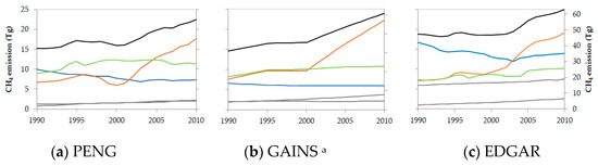
Figure 1.
a GAINS provides emission data in snapshots of five years, and annual values were obtained from interpolation. CH4 emission inventory data during the years 1990–2010 compiled from the existing CH4 inventories: black—all sectors; blue—rice cultivation; green—livestock; orange—coal mining; grey—minor sources; left y-axel—sectorial CH4; right y-axel—total CH4. (a) PENG; (b) GAINS; (c) EDGAR.
PENG [11] reports that the amount of CH4 emissions during the years 1980–2010 increased from 24.4 Tg in 1980 to 30.3 Tg in 1990, and reached 44.9 Tg in 2010, meaning that the average annual increase rate during that period was 2.1%. Until the year 1992, rice cultivation was the major contributor of CH4 emissions, but it was outpaced by livestock emissions during the years 1993–2004. However, livestock emissions slightly decreased from 2005 to 2010. CH4 from coal mining has increased significantly since 2000, and since the year 2005 onward it has overtaken rice cultivation and livestock to become the highest emitter.
GAINS [12] reports, the amounts of CH4 emissions since 1990 and will continue until 2030. Emissions have been rising from 30.8 Tg in 1990, to 50.6 Tg in 2010, with an average annual increase rate of 2% and an expectation that they will reach 67.4 Tg by 2030. The top three major emitters were coal mining, livestock, and rice cultivation, sequentially, for all years. GAINS reports that CH4 emissions from coal mining have sharply increased over time, and that since 2000 it has become the highest emitter, while CH4 emissions from livestock have slightly increased and consistently remained the second highest emitter since 2000 CH4 emissions from rice cultivation have shown a slight decrease since the year 1990.
EDGAR [10] reports, CH4 emissions from 1970 to 2012, and a growth from 47.3 Tg in 1990, to 63.2 Tg in 2010, with the average annual growth rate about 1%. During the years 1970–2002, the main CH4 contributors in China were rice cultivation, livestock, and domestic sources, though wastewater and the coal mining sector levels were close behind. Fugitive CH4 emissions from coal mining have increased since 1970, and significantly outpaced those of other sources such as wastewater in the year 1978 and the residential sector in the year 1989. Presently, CH4 emissions from coal mining have become the highest contributor of emissions since the year 2003 onward.
These results demonstrate that all inventory sets report similar data, indicating that CH4 emissions in China tend to continuously rise with different annual growth rates at 2.1%, 2.0%, and 1.0% for PENG, GAINS, and EDGAR, respectively. Although EDGAR showed the lowest annual growth rate, the annual amount was significantly higher (i.e., it was 35% and 30% above that of PENG and GAINS, respectively). Recall that this version of EDGAR (EDGAR v.4.3.2) was developed from more-updated information compared with the previous version (EDGAR v.4.2FT). Thus, the results of EDGAR v.4.3.2 present lower amounts than EDGAR v.4.2FT by about 6–19%, with significant decreases in the coal mining sector (27–39% decrease from the previous version) and moderate decreases in the livestock sector (0–14% decrease) and rice cultivation sector (0–9% decrease). Meanwhile, there were significant increases in the residential sector (18–39% increase) and wastewater sector (7–14% increase). EDGAR v.4.3.2 reports a lower amount than the previous EDGAR (EDGAR 4.2 FT). Even so, their values are still higher than other bottom-up inventories. This information emphasizes the research results of Thompson et al. [5] and Prabir et al. [6], both of whom have reported the overestimation of EDGAR 4.2FT in China.
When taking into consideration CH4 emissions by source, all three inventory data sets show that the main contributors to CH4 emissions were coal mining, livestock, and rice cultivation. These three activities accounted for about 70–80% of the overall CH4 emissions in China. Before the year 2000, agricultural activities such as rice cultivation and livestock activities were the main contributors, but the exact ranking showed some sequential alternations among data sets. After the year 2000, fugitive emissions from coal mining increased significantly and this source became the highest emitter, overtaking rice cultivation and livestock activities during the years 2003 and 2005, respectively. Meanwhile, emissions from rice cultivation were rather stable and tended to show slight decreases. For the minor sources of CH4 emissions in China, all studies reported similar findings, in that the minor sources included fugitive emissions from oil and gas, waste (municipal solid waste and wastewater), residential activities, and residue burning with different rankings. Although, all sets reported consistency in regards to emission trends, sector magnitudes were significantly different, as summarized in Table 2. The largest difference was found for rice cultivation, as presented in Figure 2a, for which EDGAR reported the highest amounts at 80% and 54% difference from GAINS and PENG, respectively. The second largest difference was found for the coal mining sector, as presented in Figure 2b, for which GAINS reported the highest amounts at 7% and 24% difference from EDGAR and PENG, respectively, while EDGAR reported a value about 15% higher than that of PENG. For CH4 from the livestock sector, there were insignificant differences, especially between EDGAR and GAINS, for which only a 3% difference was detected as presented in Figure 2c.
Table 2.
Amounts and difference of CH4 emissions during 1990–2010 among the existing sets of CH4 emission inventories.
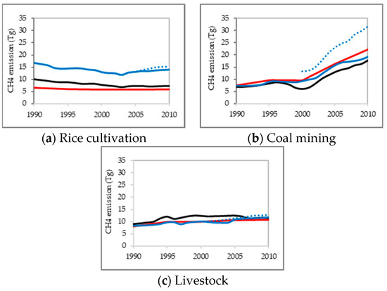
Figure 2.
Comparison of CH4 emissions by major contributors: black line—PENG; red line—GAINS; full blue line—EDGAR v. 4.3.2; dot blue line—EDGAR v.4.2. (a) rice cultivation sector; (b) coal mining sector; (c) livestock sector.
The parametric variability uncertainty was analyzed in order to identify the causes of the differences among the results for the three sets of inventories. From the analysis based on the variation of only activity data parameters (AD), only emission factor parameters (EF), and all parameters related to emission estimations (All) for the year 2010 in each sector, we found that the rice cultivation sector had the largest uncertainty, at a value of 106%, because of the variation of all parameters in this sector (Figure 3). Coal mining ranked second for uncertainty with a maximum uncertainty of 33%, and livestock had the lowest rank of uncertainty with only 12%. These results demonstrate that there were large variations in the parameters used to estimate emissions from rice cultivation among the different sets of inventories. The details of the variation for each parameter are presented in following section.
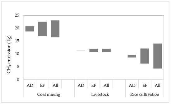
Figure 3.
Range of CH4 emissions for the year 2010 by sector based on the results from the parametric variable uncertainty analysis. AD, EF, and All refer to the parametric variability uncertainty from variationonly activity data, only emission factor, and all related parameters (both activity data and emission factor parameters) used in the calculation, respectively.
3.1. Assessment of CH4 Emissions from the RICE Cultivation Sector
In the year 2010, the total amount of rice cultivation was about 29.9 million ha, which were mainly planted in the East region of China. However, during the past 20 years, the rice cultivation area in China has declined from 33.1 million ha in 1990, with the lowest level at 26.5 million ha in 2003 [20]. The most significant decreases occurred in Gansu, Guangdong, Zhejiang, and Fujiang, but the plantation area also increased in some provinces including Jiangsu, Heilongjiang, Shandong, and Anhui [21]. Rice cultivation patterns in China can be classified by seasonality into four types, namely, early, middle, single-late, and double-late rice, in which middle rice represents the major cultivation season [22]. Early rice is planted from February to April, and harvested from June to July. Middle and single-late rice are planted from March to June, and harvested from October to November. Double-late rice represents the second round of rice cultivation, and is planted after harvesting the single-late rice [21]. Rice cultivation patterns in China vary by region because of the different topography and weather among regions [22]. CH4 emissions from rice cultivations occur after the anaerobic decomposition of organic material, and are emitted into the atmosphere [23,24]; these emissions can be estimated from the function of the harvested area, plantation period, and emission factor for different rice cultivation systems, as presented in Equation (3) [25].
where is the annual methane emission from rice cultivation, is the annual harvested area of rice for i, j, k conditions, represents the cultivation period of rice for i, j, k conditions, is a daily emission factor for i, j, k conditions, and i, j, k represent different ecosystems, water regimes, types of systems, amounts of organic amendments, and other conditions.
Table 3 presents a summary of the values and references used in the existing inventories by parameter, and further details are as follows.
Table 3.
Summary of references, data, and data variability used in the sets of inventories for the rice cultivation sector.
Annual harvested area : PENG references the annual rice cultivation area by province via the China Statistical Yearbook [11]. GAINS and EDGAR reference a similar source that uses statistics from the Food and Agriculture Organization (FAO) [14,16]. By taking into consideration the statistics from the two references found in the records between the years 1990 and 2010, the difference in values was found to be about 2% to 4%, respectively.
Cultivation period : The cultivation period depends on seasonality. PENG references the study of Yan et al. [26], who used 77, 110–130, and 93 days for early, middle, and late rice, respectively [11]. GAINS relied on a unique assumption, which assumed a value of 185 days [14]. EDGAR references the study of Neue [17], in which the cultivation period was given in the range of 83–110 days as the minimum and maximum, respectively, and 100 days was given as the median [27].
Rice ecosystem (i,j,k): PENG considers four conditions for rice ecosystems, including (1) regionality (five regions according to the FAO agricultural ecosystem zoning), (2) seasonality (early, middle, late), (3) flooding pattern (intermittent flooding (IR) and continuous flooding (CF)), and (4) use of organic amendments (OM). For the first two conditions, PENG references information from the China Statistical Yearbook, while for the third condition, values from Yan et al. [26] at the rate 66.7% and 33% of the total area for IR and CF fields, respectively, were used, with a unique assumption set for the last condition [11]. GAINS considers only the water regime condition, and data are classified into three rice ecosystems, namely, continuously flooded, intermittently flooded, and upland fields. For each type of system, proportions were drawn from the International Rice Research Institute (IRRI) [14], in which the share between IR and CF is at 40% and 60%, respectively [12]. EDGAR classifies ecosystems as rainfed, irrigated, deep water, and upland, for which the proportions of each type of system are taken from the similar references used in GAINS [16]. These findings indicate that GAINS and EDGAR consider only water regime condition which is the main factor that has a significant influence on the emissions in rice cultivation [27,28,29,30]. However, there use the higher proportion of continuous flood, in which this condition has the higher EF than intermittent flood conditions.
Emission factor : the value of the EF depends on the rice ecosystem considered. PENG considers four aspects of rice ecosystems—regionality, seasonality, water regime, and fertilizer use—and so the EFs used in PENG vary in accordance with these rice ecosystem conditions, data on which were obtained from the study of Yan et al. [11,26]. In that study, zonal/regional EFs are provided that are disaggregated by cultivation conditions into 36 categories in the unit of mg CH4/m2/h, for which the range amounts to 0.12–4.51 kg/ha/day for IR fields with OM, and 1.68–6.07 kg/ha/day for CF fields with OM [26]. GAINS references the default value for the EF from the 2006 IPCC GLs together with theirits own assumption [14]. The 2006 IPCC GLs provide an EF for the baseline condition which involves continuous flooding without OM at 1.3 kg/ha/day [25]. GAINS assumes that the EF for continuous flooding conditions is two times that of intermittent flood conditions [14], so the EF for the intermittent flood condition is about 0.65 kg/ha/day. In EDGAR, the study of Neue [27] is referenced, in which the emission flux for irrigated fields in China is given as 0.6–14.1 kg/ha/day (3.4 kg/ha/day for the median rate) [27]. Thus, it can be seen that the lower range of Neue [27] associates with the EFs of GAINS for the intermittent conditions, whereas the middle value correlates with (or rather is higher than) the EFs of GAINS in the case of continuous flooding conditions. By taking into consideration the EF for the major type of rice ecosystem in China, which is the middle rice type according to the study of Yan et al. [26], the average regional EF values under this condition are in a range of 0.09–2.81 kg/ha/day for intermittent floods, and 1.26–4.56 kg/ha/day for continuous flooding. EF varies by zone, as presented in Figure 4, and the highest rate occurs in zone AEZ6B (covering the area of the Southwest region), while the lowest rate occurs in zone AEZ8 (covering the area of the North region). Following the conversion of the regional EFs to a national EF by weighting with the provincial paddy field area found, the national EF rate was found to be about 1.95 kg/ha/day. By comparing these ranges with the EF rates used in GAINS and EDGAR, we found the national EF was about 33% higher than the default value of the 2006 IPCC GLs (used in GAINS), whereas it was 74% lower than the middle rate of Neue [27], which is referenced in EDGAR.
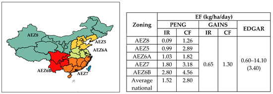
Figure 4.
Emission factors for rice cultivation used in the existing inventory.
As the details of each parameter used in each set of inventories demonstrates, EDGAR reported the highest amount of CH4 because of its use of a higher proportion of the main emitter as the continuous condition combined with the use of higher-rate EFs compared with those of GAINS and PENG. Meanwhile, GAINS used the same share of continuous flooded fields as EDGAR (which was 26.7% higher than that of PENG), with a lower rate of EFs (which were about half of the EFs of Yan et al. in the case of middle rice), and as a result, it reported the lowest amount of CH4 emissions. With the variation of all parameters, there was a resulting uncertainty in the emission estimations of about 85%–106% uncertainty, which amounts to CH4 emissions in the range of 4.3–16.9 Tg. The lower bound was obtained from assuming the paddy field area from the China Statistical Yearbook, combined with assigning the proportion of continuous flooding at 40% of the total rice cultivation area (as used in PENG) with an EF of 1.3 kgCH4/ha, as representative of the continuous flooding conditions, with or without OM, as used in GAINS. The upper bound was obtained from the statistical data on the paddy field area from the FAO, combined with a designation of 60% continuous flooding and a maximum rate of the daily EF (14.1 kgCH4/ha), as referenced in EDGAR.
The temporal allocation of emissions data, which only EDGAR considered, showed that the highest emissions occurred during February–April (more than one-third of the annual emissions) and August–October (about a quarter of the annual emissions), for which the largest share occurred in March (16% of annual emissions). The first peak period corresponds with the early rice cultivation season, whereas the latter peak period matches the late rice plantation season. This means that the temporal distribution from EDGAR represents areas that can plant two or three crops per year, and that only the southern and central regions have double harvests [31]. This temporal distribution is unrepresentative of the single crop plantation areas, which mainly planted in North, Northeast, and Northwest regions. In addition, the peak emissions reported by EDGAR are slightly different from the results of Yan et al. [26], who reported that CH4 emissions from rice cultivation start in March and are continuous throughout the fallow season, during which emissions will become highest from June to July (about 40% of the annual emissions) in consideration of the seasonality of rice as early, middle, and late rice cultivation periods [26].
3.2. Assessment of CH4 Emissions from the Coal Mining Sector
China is one of the world’s major coal producers [32]. According to records of the US Energy Information Administration (EIA), about 12,000 coal mines are in operation in China (as of 2014), and these are mainly bituminous coal operations, with only some involving anthracite and lignite. These mines are located in 28 provinces, particularly in the North region, except for the anthracite mines, which are mostly found in the Central region [32]. About 17% of the mines belong to state-owned coal mine groups (which accounts for a total of 61% of coal production), and 83% of mines are owned by villages and towns (which account for about 39% of coal production) [33]. Most of the mines in China are underground mines, and there are only a few open pit mines [33]. Both types of active coal mines have emissions from four sources, including mining (ventilation and degasification), post mining (handling, transport, and storage), oxidation, and uncontrolled combustion (the fires that occur from the heat), which are significantly higher in underground mines [34]. Mining and post mining activities are the major sources of CH4 emissions, for which the quantity mainly depends on the ranking of coal and the mining depth [35,36]. The 2006 IPCC GLs [34] provide the principles for estimating fugitive emissions from coal mining for Tier 1 and Tier 2 levels, as presented in Equation (4), and these emissions are based on the amount of raw coal production by mine types, the EF for each process and each mine, and the CH4 recovery.
where Ei,j is the sum of emissions from all mines (i) for all processes (j), ADi is the amount of raw coal production by mine type i (surface (S)/underground (UG)), EFi,j is the CH4 emission factor by mine type i and process j (mining/post mining), and CH4rec is the CH4 recovered and utilized for energy production or flared.
Table 4 summarizes the values and references for each parameter used for coal mining emission estimations in the existing inventories, with further details are provided below.
Table 4.
Summary of references, data, and data variability used in sets of inventories for the coal mining sector.
Amount of coal production by mine type (ADi): PENG uses the amount of coal production at the provincial level obtained from the China Statistical Yearbook, and disaggregates coal production into underground and surface mines at rates of 95% and 5%, respectively, for which data were obtained from the provincial average [11]. GAINS uses data at the national level obtained from the World Energy Outlook of the International Energy Agency (IEA-WEO), which assumes all coal is from underground mining [14]. EDGAR uses the amount of coal production from the IEA and disaggregates data into surface and underground mines based on information from the World Coal Association [16]. From this information, the variation of activity data occurred from two points—the total amount of coal production, and the share of mine types. In regard to the amount of coal, two references are used (the China Statistical Yearbook and the IEA). Both references provide consistent information, in which there is only a 0–5% difference for the overall amount of coal production during the years 1990–2010. This variation arose from the unit conversion process. The China Statistical Yearbook provides the amount of coal production in units of coal equivalents (Coe) [37], while the IEA provides two units, namely, ton of oil equivalents (toe) and heating values (PJ) [38]. Regarding share of mine types, there is a 5% difference in underground mines, for which PENG assumed the lower share, and a 100% difference in surface mines, for which only PENG assigns a rate.
Emission factor of underground mining (EFUG-mine): PENG uses seven regional EFs in the range of 5.58–20.35 m3/t, as summarized in Figure 5, for which the characteristics of mines are identified as depth and coalbed methane, with reference to Zheng et al. [36]. The high rate (20.35 m3/t) is assigned to the provinces in the Southwest region, which accounted for about 13% of the total coal production in 2010, and the low rate (5.58 m3/t) is assigned to the provinces in the North region, which accounted for about 45% of coal production the same year. With the regional EFs used in PENG and the regional coal production in the year 2010, the weight average of EF was determined to be about 8.2 m3/t. GAINS has a value of 9.3 m3/t, which was obtained from modifying the lower bound of the default value of the 2006 IPCC GLs and based on information from China University of Petroleum to be consistent with the characteristics of mines [14]. EDGAR references the lower bound of the EF from EMEP/EEA [16], for which EMEP also used IPCC guidelines for GHG emissions as representative values to calculate emissions [39]. This rate was down from the previous version (EDGAR v.4.2FT), which used the European average EFs in cases of missing data [40], and these were about two times higher for coal mining in China [35]. The 2006 IPCC guidelines proposed the default value for underground mining as 10–25 m3/t [34]. Utilizing this information, we can see that the EF rate referenced in EDGAR is slightly higher than the EF rate used in GAINS and PENG; specifically, it is higher by about 7% and 17%, respectively. However, with the various mining characteristics of coal mines in China, the uncertainty of the EF between the regional-level EF (used in PENG) and country-level EF (used in EDGAR and GAINS) reaches a difference of about −79% to 54%, which is the result of lower estimations in the Southwest region and an overestimation of the North region, since the country-level EF is used. These results correlate with the inversion results by Thompson et al., which found high emissions in Shaanxi [5], a province in the North region.
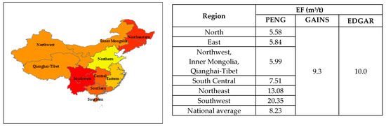
Figure 5.
Emission factors for underground mining used in the existing inventories.
Emission factor of post underground mining (EFUG-post mine): PENG uses a rate in the range of 1.18–1.30 m3/t, which was obtained from modifying of the default value of the 2006 IPCC GLs together with the average weight of coal production [11]. GAINS uses a value of 2.5 m3/t, which was referenced from the median rate of the 2006 IPCC GLs [14]. EDGAR references the lower bound of the default value given in the 2006 IPCC GLs [16], for which the rate was set at 0.9 m3/t [34]. The default value of the 2006 IPCC GLs was in the range of 0.9–4.0 m3/t. These findings demonstrate that the EF used in PENG is rather close to the lower bound of the IPCC 2006 guidelines, which are referenced in EDGAR, while the EF rate used in GAINS is rather higher than those used in the other studies.
Emission factor of surface mines—mining (EFS-mine): only PENG considers some of coal production obtained from surface mines which the proportion of surface mining at 5% of coal production. PENG uses an EF of surface mines—mining at 2.5 m3/t, which was modified from the default value of the 2006 IPCC GLs [11].
Emission factor of surface mines—post mining (EFS-mine): information is unclear on the EF of the surface mines—post mining activity used in PENG. However, the EF for this portion is very small compared with the mining stage, as the default value from the 2006 IPCC GLs was only 0–0.2 m3/t [34].
The rate of CH4 recovery used in each set of inventories: PENG assumes the recovery rate changed over the years at a rate of 3.59–9.26% using data that were modified based on Zheng et al. [36], the growth of the economy, and the use of more intensive safety measures [11]. GAINS references the recovery rate from the USEPA at 12%, and uses a constant rate for all years [14]. EDGAR references the rate from Cheng et al. at 9.0% [16,17]. This information demonstrates that the recovery rates used in each set are quite consistent, with GAINS reporting the highest rate, while EDGAR reports nearly the same rate as PENG for the year 2010.
As the details of each parameter used in each set of inventories demonstrate, GAINS produces the highest results due to using the higher proportion of underground mines in conjunction with a higher EF rate of underground coal-post mining. Meanwhile, EDGAR reports the second highest findings of CH4 emissions, which are closer to the results from GAINS than from PENG, because of the closer resemblance in the EF-underground mining between EDGAR and GAINS in which higher rate than PENG used. PENG has the lowest findings of CH4 emissions, due to using the lower proportion of underground mine (which is the main emitter of coal mining), combined with the lowest EFs when converting regional EFs to national EFs (which are equivalent to those of other studies). With the variation of all parameters, there is an uncertainty of emission estimations of about 10%–33%, which accounts for CH4 emissions in the range of 16.4–23.0 Tg. The lower bound of emissions was obtained by assuming the proportion of underground to surface mines at 95–5% (as used in PENG) and the average-weight regional EFs from PENG, combined with the highest recovery rate at 12%, as referenced in GAINS. Meanwhile, the upper bound was obtained by including all underground mines (as used in GAINS and EDGAR), as well as the low EF from the 2006 IPCC GLs and the recovery rate used in EDGAR.
3.3. Assessment of CH4 Emissions from the Livestock Sector
CH4 emissions from livestock are composed of emissions from fermentation and manure management, which are related to the digestive processes of ruminant and non-ruminant animals, as well as the decomposition of animal urine and dung under anaerobic conditions. The amount of CH4 from livestock depends on several factors, such as the animal type, animal characteristics (age, sex, weight), animal performance, food intake characteristics (type, quantity, and quality), and so on [25]. The 2006 IPCC GLs [25] provide the principles for estimating CH4 emissions from livestock in Tier 1 and Tier 2, as presented in Equation (5), in which the accuracy of the estimation depends upon the details of the parameters used for EF derivation. For the Tier 1 method, only animal characteristics and average annual temperatures (for manure management) are considered when determining the EF, whereas the Tier 2 method determines the EF based on animal and food characteristics to estimate enteric fermentation emissions and manure and manure system characteristics to estimate manure management emissions. For the Tier 3 method, more country-specific details are considered, such as dietary compositions, seasonal variation in animal populations, feed quality, and so on, and these data are mainly obtained from direct measurements [25].
where Ei is the sum of emissions from enteric and manure management for all types of animals, Ni is the number of heads for animal type/sub-type i, is the enteric methane emission factor for livestock type/sub-type i, is the manure management emission factor for livestock type/sub-type i, and is the amount of biogas utilization.
Table 5 summarizes the values and references used for each parameter for livestock emission estimations used in the existing inventories, and further details are provided below.
Table 5.
Summary of reference, data, and data variation used among sets of inventories in the livestock sector.
Number of animals (Ni): PENG estimates emissions for six types of animals (dairy cattle, nondairy cattle, buffalo, sheep, goat, and swine), in which the number of animals at the end of the year is referenced by province from the China Statistical Yearbook. These data consider slaughtered and live animals in which details on sex, age, and manure characteristics are provided [11]. GAINS estimates emissions for eight types of animals (the same as above plus camels and horses) by referencing FAO statistics (FAOSTAT), which take into consideration detailed information for dairy cattle [14]. EDGAR estimates emissions for 11 types of animals (the same as GAINS plus mules, assess, and poultry) by referencing FAOSTAT [16]. By taking into consideration statistics for the total heads of cattle and buffalo, which are the major types of large animals in the China Statistical Yearbook and FAOSTAT, we found that the numbers from the two statistics were rather consistent, with only a 0.1%–1% difference.
Emission factor of enteric fermentation : PENG computes EFs disaggregated into three categories, namely, mature females, young, and others, by using average values from previous studies including the default value in the 1996 IPCC GLs and the 2006 IPCC GLs [11]. GAINS uses the default value from the country report submitted to the United Nations Framework Convention on Climate Change (UNFCCC) together with the default value of the 2006 IPCC GLs, for which data were identified by animal type, with detailed information provided for dairy cows and adjustments to the EF based on milk production [12,14]. EDGAR references the default value of the 2006 IPCC GLs, which considers the country-specific milk yield for dairy cattle and carcass weight for non-dairy cattle [16,17]. By taking into consideration the rate of the EF for dairy cattle, non-dairy cattle, and buffalo (which are the major sources of livestock emissions) under the same animal characteristics in each study, we found that the rates had slight differences. The EF of dairy cattle from the 2006 IPCC GLs used in EDGAR was slightly higher than the EFs used in GAINS and PENG. The EF of non-dairy cattle from the 2006 IPCC GLs used in EDGAR was in the range between GAINS and PENG. The EF of buffalo from the 2006 IPCC GLs used in EDGAR is rather lower than the rate in PENG.
Emission factor of manure management : PENG uses the default value of the 2006 IPCC GLs, which identified the average annual temperature rate by province [11]. GAINS modifies the default value of the 2006 IPCC GLs based on the average national temperature [14], for which the EF, at a temperature of 18 °C, is rather close to the rate that PENG identifies for provinces in the East and Central regions. EDGAR references the default value of the 2006 IPCC GLs by using zoning temperatures [17].
CH4 utilization : methane from manure management is widely used in the form of biogas. PENG references the study of Feng et al. [41], along with the number of household bio-digesters, to quantify the amount of biogas. It assumes the proportion of biogas accounted for by manure management under three scenarios to be in the range of 10%–25%, based on Yin [42]. GAINS considers three scales of anaerobic digestion plants, including farm, household, and community scales [14]. However, GAINS identifies the non-utilization of biogas in the case of China, based on the information of An et al. [43]. It also notes the intensity of labor costs to operate digester systems, which are rather impossible to implement in certain countries that have low average wage rates in agriculture (including China) [9,14]. There is no statement about the utilization of biogas reported in EDGAR.
As the details for each parameter used in each set of inventories show, all sets used a similar basis in terms of IPCC data, with some different details for activity data, which led to different EF rates being used. From the variation of all parameters, the amount of CH4 can be expected to be about 10.5–12.0 Tg, or 0.002%–12% parametric variability uncertainty. The upper bound was obtained by using the default enteric EF from the 2006 IPCC GLs for dairy cattle (as used in EDGAR), and from PENG for non-dairy cattle and buffalo, along with the EF of manure management from PENG. The lower bound was obtained using the default enteric EF from PENG for dairy cattle, and the default value of the 2006 IPCC GLs for the rest of the activities. The often low uncertainty can be attributed to the proximity of values used in each of the data sets, which resulted in small differences in the results among the existing inventories.
4. Conclusions
This study aimed to investigate the uncertainty of bottom-up emission estimations, as implied in the inverse modeling results, by using parameter variability uncertainty analysis. Three sets of inventories were considered in this study, namely, one that covered the national level of China called PENG, and two remarking on the international level that also provided data for China called GAINS and EDGAR. Based on the parameter variability uncertainty analysis in the main contributor sectors, we found that the largest uncertainty occurred in the rice cultivation sector, followed by the coal mining sector and livestock sector. By taking into consideration the causes of the uncertainties by sector, we found that the uncertainty in the rice cultivation sector came from the differences in the proportion of the water regime used in combination with the variation of EFs specified for each rice ecosystem. The higher share of continuously flooding land, along with the higher EF rates used in EDGAR, were key reasons why the results of EDGAR were higher compared to those of the other inventory sets. The higher share of continuously flooding fields together with the lower EFs for all ecosystems used in GAINS led to GAINS having the lowest result of emissions. For coal mining, the uncertainty of emission estimates was mainly caused by the variation of EFs, which were rather lower rate in PENG either of the EFs of mining or post mining for underground (UG) mines. The higher share of underground mines along with the higher EFs used in GAINS, especially for underground post mining, were the main reasons for it having the highest results. EDGAR produced results rather close to those of GAINS due to similarities in the assumption of the activity data and similar EFs. Less uncertainty was found for the livestock sector, but some differences were caused by the details included in the activity data among the different sets of inventories.
Results of this study imply that overestimations of CH4 emissions in China, as inferred by inverse modeling studies, are due to uncertainties in emission estimates, particularly in regard to emission factors for the rice cultivation and coal mining sectors. However, it is currently not easy to determine which factor is more influential. There should be differences in spatial and temporal variations of emissions in these sectors. If more detailed information in terms of finer spatial and temporal variations in emissions can be derived from inverse modeling, these data would be quite useful for obtaining a better understanding of the influencing factors.
There are numerous studies that apply bottom-up and top-down methods for emission estimates. Presently, there is an urgent need to obtain deep understandings on variations in such data for establishing better emission inventories. While an investigation like this study is not sophisticated, the approach can be useful for validating and improving emission estimates. Such research will lead to more confidence about NDC achievements and progress toward sustainable development.
Author Contributions
P.C. and S.C. designed the study in conjunction with conceptual advisement provided by N.S., P.C. and S.C. collected and investigated all of the information related to this study. P.C. wrote the manuscript in conjunction with advisement provided by S.C. and N.S. All authors discussed the results and contributed to the final manuscript.
Funding
This research was supported by the Environment Research and Technology Development Fund (2-1701) of the Environmental Restoration and Conservation Agency.
Acknowledgments
The authors would like to sincerely thank Lena Hoglund-Isaksson, Sushi Peng, and the IIASA-team for providing information and valuable suggestions during this study.
Conflicts of Interest
The authors declare no conflict of interest.
References
- Kirschke, S.; Bousquet, P.; Ciais, P.; Saunois, M.; Canadell, J.G.; Dlugokencky, E.J.; Bergamaschi, P.; Bergmann, D.; Blake, D.R.; Bruhwiler, L.; et al. Three decades of global methane sources and sinks. Nat. Geosci. 2013, 6, 813–823. [Google Scholar] [CrossRef]
- Turner, A.J.; Frankenberg, C.; Wennberg, O.P.; Jacob, J.D. Ambiguity in the causes for decadal trends in atmospheric methane and hydroxyl. PNAS 2017, 114, 5367–5372. [Google Scholar] [CrossRef] [PubMed]
- Bergamaschi, P.; Corazza, M.; Karstens, U.; Athanassiadou, M.; Thompson, R.L.; Pison, I.; Manning, A.J.; Bousquet, P.; Segers, A.; Vermeulen, A.T.; et al. Top-down estimates of European CH4 and N2O emissions based on four different inverse models. Atmos. Chem. Phys. 2015, 15, 715–736. [Google Scholar] [CrossRef]
- Bergamschi, P.; Howeling, S.; Segers, A.; Krol, M.; Frankenberg, C.; Scheepmaker, A.R.; Dlugokencky, E.; Wofsy, S.C.; Kort, E.A.; Sweeney, C.; et al. Atmospheric CH4 in the first decade of the 21st century: Inverse modelling analysis using SCIAMACHY satellite retrievals and NOAA surface measurements. J. Geogphys. Res. 2013, 118, 7350–7369. [Google Scholar]
- Thompson, R.L.; Stohl, A.; Zhou, X.L.; Dlugokencky, E.; Fukuyama, Y.; Tohjima, Y.; Lee, H.; Nisbet, G.E.; Fisher, E.R.; Lowry, D.; et al. Methane emissions in East Asia for 2000–2011 estimated using an atmospheric Bayesian inversion. J. Geophys. Res. 2015, 120, 4352–4369. [Google Scholar] [CrossRef]
- Prabir, K.P.; Saeki, T.; Edward, J.; Kencky, D.; Ishijima, K.; Umezawa, T.; Ito, A.; Aoki, S.; Morimoto, S.; Crotwell, A. Regional methane emission estimation based on observed atmospheric concentration (2002–2012). J. Meteorol. Soc. Jpn. 2016, 94, 85–107. [Google Scholar]
- IPCC. 2006 IPCC Guidelines for National Greenhouse Gas Inventories, Prepared by the National Greenhouse Gas Inventories Programme; Eggleston, H.S., Buendia, L., Miwa, K., Ngara, T., Tanabe, K., Eds.; IGES: Hayama, Japan, 2006. [Google Scholar]
- Janssens-Maenhout, G.; Dentener, F.; van Aardenne, J.; Monni, S.; Pagliari, V.; Orlandini, L.; Klimont, Z.; Kurokawa, J.; Akimoto, H.; Ohara, T.; et al. EDGAR-HTAP: A Harmonized Gridded Air Pollution Emission Database Based on National Inventories; JRC Scientific and Technical Reports; EUR Report No. EUR 25299-2012; European Commission Joint Research Center Institute for Environment Sustainability: Ispra, Italy, 2012. [Google Scholar]
- Global Emission EDGAR v4.2 FT 2012. Available online: http://edgar.jrc.ec.europa.eu/overview.php?v=42FT2012 (accessed on 23 March 2019).
- Global Greenhouse Gases Emissions EDGAR v4.3.2. Available online: http://edgar.jrc.ec.europa.eu/overview.php?v=432_GHG&SECURE=123 (accessed on 23 March 2019).
- Greenhouse Gas—Air Pollution Interactions and Synergies—Asia (GAINS Asia). Available online: https://gains.iiasa.ac.at/gains/emissions.ASN/index.menu?open=none&switch_version=GAINS&switch_lang=lang_en (accessed on 23 March 2019).
- Shushi, P.; Shilong, P.; Philippe, B.; Philippe, C.; Bengang, L.; Xin, L.; Shu, T.; Zhiping, W.; Yuan, Z.; Feng, Z. Inventory of anthropogenic methane emissions in mainland China from 1980 to 2010. Atmos. Chem. Phys. 2016, 16, 14545–14562. [Google Scholar]
- ECLIPSE-Evaluating the Climate and Air Quality Impacts of Short-Lived Pollutants. Available online: http://eclipse.nilu.no/language/en-GB/Home.aspx (accessed on 21 January 2019).
- Hoglund-Isaksson, L. Global anthropogenic methane emissions 2005–2030: Technical mitigation potentials and costs. Atmos. Chem. Phys. 2012, 12, 9079–9096. [Google Scholar] [CrossRef]
- European Commission. Joint Research Center: EDGAR-Emissions Database for Global Atmospheric Research. Available online: http://edgar.jrc.ec.europa.eu/# (accessed on 21 January 2019).
- Janssens-Maenhout, G.; Crippa, M.; Guizzardi, D.; Muntean, M.; Schaaf, E.; Dentener, F.; Bergamaschi, P.; Pagliari, V.; Olivier, J.G.; Peters, J.A.; et al. EDGAR v4.3.2 Global Atlas of the three major Greenhouse Gas Emissions for the period 1970–2012. Earth Syst. Sci. 2017, 10. [Google Scholar] [CrossRef]
- JRC Ispra-IES; Janssens-Manhout, G.; Guizzardi, D.; Bergamaschi, P. Informative Note of the Emission Inventory Compiled by EDGAR Using also EPRTR Data for the INGOS Project. Available online: http://edgar.jrc.ec.europa.eu/docs/Informative_note_on_the_Emission_inventory_compiled_by_EDGAR_for_INGOS.pdf (accessed on 5 April 2019).
- Morris, D.M. Factorial Sampling Plans for Preliminary Computational Experiments. Technometrics 1991, 33, 161–174. [Google Scholar] [CrossRef]
- Campolongo, F.; Cariboni, J.; Saltelli, A. An effective screening design for sensitivity analysis of large models. Environ. Model. Softw. 2007, 22, 1509–1518. [Google Scholar] [CrossRef]
- China Agricultural Statistical Yearbook (CASY). 1980–2010 China Statistics; Agriculture Press: Beijing, China, 1990–2010. [Google Scholar]
- Liu, Z.; Li, Z.; Tang, P.; Li, Z.; Wu, W.; Yang, P.; You, L.; Tang, H. Change analysis of rice area and production in China during the past three decades. J. Geogr. Sci. 2013, 23, 1005–1018. [Google Scholar] [CrossRef]
- Ricepedia the Online Authority on Rice: China. Available online: http://ricepedia.org/china (accessed on 27 July 2018).
- Chao, F.; Guirui, Y. Estimation and spatiotemporal analysis of methane emissions from agriculture in China. Environ. Manag. 2010, 46, 618–632. [Google Scholar]
- IPCC. 2006 IPCC Guidelines for National Greenhouse Gas Inventories; Intergovernmental Panel on Climate Change; IGES: Hayama, Japan, 2006. [Google Scholar]
- 2006 IPCC Guidelines for National Greenhouse Gas Inventories; Vol. 4. Agriculture, Forestry and Other Landuse, Chapter 5 Crop Land and Chapter 10 Emission from Livestock and Manure Management; IGES: Hayama, Japan, 2006.
- Yan, X.; Cai, Z.; Ohara, T.; Akimoto, H. Methane emission from rice fields in Mainland China: Amount and seasonal and spatial distribution. J. Geophys. Res 2003, 108, 10.1–10.10. [Google Scholar] [CrossRef]
- Neue, U.H. Flux of methane from rice fields and potential for mitigation. Soil Use Manag. 1997, 13, 258–267. [Google Scholar] [CrossRef]
- Kazuyuki, Y.; Katsuyuki, M. Effect of organic matter application on methane emission from some Japanese paddy fields. Soil Sci. Plant Nutr. 1990, 36, 599–610. [Google Scholar]
- Gon, H.A.; Neue, H.U. Influence of organic matter incorporation on the methane emission from a wetland rice field. Glob. Biogeochem. Cycles 1995, 9, 11–22. [Google Scholar]
- Wassmann, R.; Neue, H.U.; Lantin, R.S.; Buendia, L.V.; Rennenberg, H. Characterization of methane emissions from rice fields in Asia. I. Comparison among field sites in five countries. Nutr. Cycl. 2000, 58, 1–12. [Google Scholar] [CrossRef]
- FAO—Food and Agriculture Organization of the United Nations. FAO Rice Information-China, vol. 3. Available online: http://www.fao.org/docrep/005/Y4347E/y4347e00.htm (accessed on 21 January 2019).
- Energy Information Administration (EIA). International Energy Data and Analysis. Available online: https://www.eia.gov/beta/international/analysis_includes/countries_long/China/china.pdf (accessed on 5 April 2019).
- Global Methane Initiative, CMM Country Profiles: China; U.S. Environmental Protection Agency, Coalbed Methane Outreach Program: Washington, DC, USA, 2015; pp. 63–80.
- 2006 IPCC Guidelines for National Greenhouse Gas Inventories; Vol. 2 Energy, Chapter 4 Fugitive Emission; IGES: Hayama, Japan, 2006.
- Zhu, T.; Bian, W.; Zhang, S.; Di, P.; Nie, B. An Improved Approach to Estimate Methane Emissions from Coal Mining in China. Environ. Sci. Technol. 2017, 51, 12072–12080. [Google Scholar] [CrossRef]
- Zheng, S.; Wang, Y.A.; Wang, Z.Y. Methane emissions to atmosphere from coal mine in China. Saf. Coal Mines 2006, 36, 29–33. [Google Scholar]
- China Energy Statistical Yearbook (CESY). 1980–2010 China Statistics; Energy Press: Beijing, China, 1990–2010. [Google Scholar]
- IEA—International Energy Agency. World Energy Balances 2017: China Statistics 1990-2010; IEA: Paris, France, 2017. [Google Scholar]
- EEA—EMEP/EEA Air Pollutant Emission Inventory Guidebook 2013, Fugitive Emissions from Solid Fuels: Coal Mining and Handing; European Environment Agency: Copenhagen, Denmark, 2013.
- Saunois, M.; Bousquet, P.; Poulter, B.; Peregon, A.; Ciais, P.; Canadell, J.G.; Dlugokencky, E.J.; Etiope, G.; Bastviken, D.; Houweling, S.; et al. The global methane budget 2000–2012. Earth Syst. Sci. Data 2016, 8, 697–751. [Google Scholar] [CrossRef]
- Feng, Y.; Guo, Y.; Yang, G.; Qin, X.; Song, Z. Household biogas development in rural China: On policy support and other macro sustainable conditions. Renew. Sustain. Energy Rev. 2012, 16, 5617–5624. [Google Scholar] [CrossRef]
- Yin, D. The Research on Regional Differentiation of Rural Household Biogas in China and the Ratio of Raw Materials. Ph.D. Thesis, Northwest A & F University, Yangling, China, 2015. [Google Scholar]
- An, B.X.; Preston, T.R.; Dolberg, F. The introduction of low-cost polyethylene tube biodigesters on small scale farms in Vietnam. Livest. Res. Rural Dev. 1997, 9, 27–35. [Google Scholar]
© 2019 by the authors. Licensee MDPI, Basel, Switzerland. This article is an open access article distributed under the terms and conditions of the Creative Commons Attribution (CC BY) license (http://creativecommons.org/licenses/by/4.0/).