Article

Cross-Scale Water and Land Impacts of Local Climate and Energy Policy—A Local Swedish Analysis of Selected SDG Interactions

by
Rebecka Ericsdotter Engström
1,*,
Georgia Destouni
2,
Mark Howells
1,
Vivek Ramaswamy
1,
Holger Rogner
1,3 and
Morgan Bazilian
1
1
Division of Energy Systems Analysis, KTH Royal Institute of Technology, 10044 Stockholm, Sweden
2
Department of Physical Geography and Bolin Centre for Climate Research, Stockholm University, 10691 Stockholm, Sweden
3
International Institute for Applied Systems Analysis (IIASA), A-2361 Laxenburg, Austria
*
Author to whom correspondence should be addressed.
Sustainability 2019, 11(7), 1847; https://doi.org/10.3390/su11071847
Submission received: 11 January 2019 / Revised: 20 March 2019 / Accepted: 21 March 2019 / Published: 27 March 2019
(This article belongs to the Section Energy Sustainability)

Abstract

:
This paper analyses how local energy and climate actions can affect the use of water and land resources locally, nationally and globally. Each of these resource systems is linked to different Sustainable Development Goals (SDGs); we also explore related SDG interactions. A municipality in Sweden with the ambition of phasing out fossil fuels by year 2030 is used as illustrative case example. The local energy system is modelled in detail and indirect water and land requirements are quantified for three stylised decarbonisation scenarios of pathways to meeting climate and energy requirements (related to SDG13 and SDG7, respectively). Total local, national and global implications are addressed for the use of water and land resources, which relate to SDG6 for water, and SDG2 and SDG15 for land use. We find that the magnitude and location of water and land impacts are largely pathway-dependent. Some scenarios of low carbon energy may impede progress on SDG15, while others may compromise SDG6. Data for the studied resource uses are incoherently reported and have important gaps. As a consequence, the study results are indicative and subject to uncertainty. Still, they highlight the need to recognise that resource use changes targeting one SDG in one locality have local and non-local impacts that may compromise progress other SDGs locally and/or elsewhere in the world.

1. Introduction

Interrelations between the 17 global Sustainable Development Goals (SDGs) [1] are increasingly acknowledged [2,3,4]. However, each SDG is not isolated from the others and actions to meet one goal may accelerate or impede progress on others [5,6]. One example of this which is proposed for analysis of such interactions is offered by the growing number of cities developing and implementing action plans to reduce their greenhouse gas (GHG) emissions and to transform their local energy system [7,8]. While such local actions to curb global emission levels [9,10] support progress on SDG13 on “climate action” and SDG7 on “affordable and clean energy”, they also contribute to SDG11 on “sustainable cities and communities”. However, such local level initiatives may also adversely impact other resources and associated SDGs [11]. Such indirect impacts may occur both within and beyond local jurisdictional boundaries [12] with high or low visibility to local policy-makers [13].
Interactions between energy, land and water (often referred to as the food-water-energy nexus) have become an important field of sustainability research in the last decade [14,15,16,17,18,19,20]. These resource systems are complex and the various human uses of them implies impacts across the resources [21], as well as cross-regionally [22] and from local to global scales [23]. An example of such cross-scale interactions is the provision of energy in a municipality. This energy may originate from within the municipal borders and/or be traded across these and national borders. Further, energy conversions, from fuel extraction to final delivery, requires the use of water and land resources [16]. The municipal energy provision can thereby impact water and land resources locally, nationally and internationally, along the energy supply chains. Through such interconnected resource use, local energy choices may thus affect progress on SDG6 on “clean water and sanitation” and SDGs directly related to land use, such as SDG2 on “zero hunger” and SDG15 on “life on land”, with (positive or negative) impacts locally and/or remotely.
To identify and track the indirect, in addition to the direct, effects of energy provision on water and land resources, reliable data availability is crucial. While much data is reported in the literature on the use of water for energy, some aspects are more investigated and well understood than others [24,25]. Data on the water use implications of biofuels, in particular for transportation, are relatively well reported in the literature [26,27,28]. Data on the water requirements of electricity generation are also provided in several reports ([29,30] among others). However, the implications of hydropower for the consumptive use of water are debated [21]. Recent work has shown them to be considerably higher than previously assumed in relation to an associated freshwater planetary boundary [23] and to the estimated global human water footprint [31]. Data on the land requirements, in general or by type of land, for specific energy carriers are available from international institutions, industry and the scientific literature [32,33,34,35,36,37].
Cross-scale and multi-resource interactions and implications are less explored. Life-cycle assessments (LCA) consider embedded resource use in energy commodities [38,39,40], but typically focus on one or few fuels. Where the LCA scope has been broadened to include multiple fuel/energy uses, it only considers the GHG emissions of the local energy use [41]. The impacts of national energy use on global freshwater resources have been studied [42], but the implications of future developments of these resource systems are then not assessed. A British study has explored the potential impacts on land use for selected future scenarios of replacing fossil energy, but it did not quantify impacts beyond the national borders [43]. The recently launched ‘Urban Climate Action Impacts Framework’ [44] suggests a broad approach to assessing impacts of climate actions, but does not provide details on how to measure action scale or magnitude. In summary, there has been a lack of research on future development scenario implications for multiple resource uses across local, national and continental borders.
This paper aims to fill aspects of this cross-resource and cross-scale research gap by quantifying local-to-national-to-global impacts on water and land resources of local choices and pathways to energy system transformation. The Swedish municipality of Oskarshamn is used as a case study, with relevant available data, for this investigation. Sweden has repeatedly been top-ranked in world assessments of progress towards meeting the SDGs [45,46,47], with local level actions playing a key role for such progress [48]. Sweden has also been recognised as a top ranking country by [49], when correlating high Human Development Index with relatively low emissions. In Sweden, the municipality of Oskarshamn is an ambitious local actor in this context, for example joining the Covenant of Mayors in 2011 [50]. In compliance with this commitment, the municipality aims to eradicate the use of fossil fuels by 2030, and reduce local (fossil) CO2 emissions to zero [51]. In this paper, we analyse different possible pathways to reaching these aims and associated local to global implications for water and land resources.

2. Materials and Methods
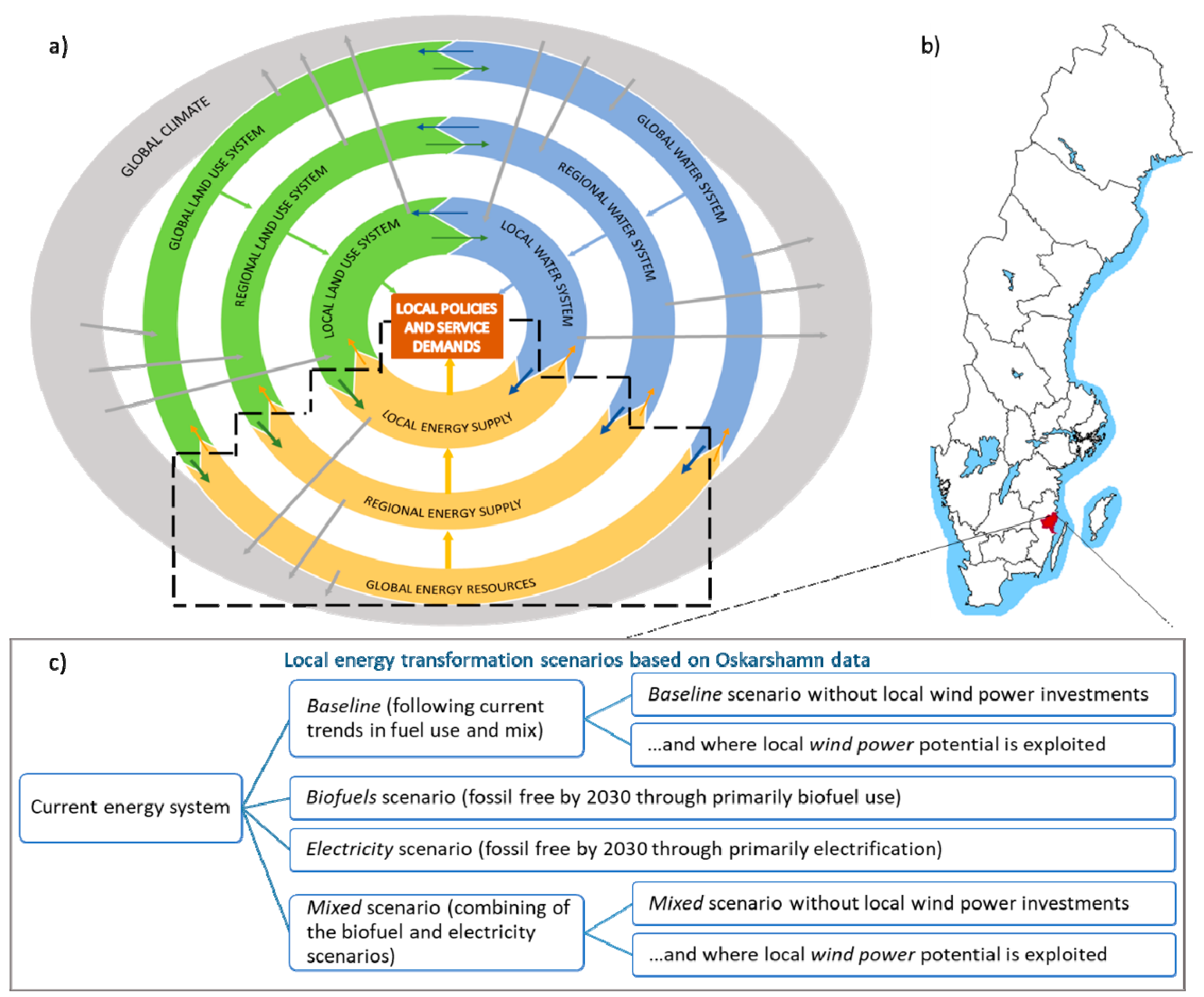
2.1. Study Area

The municipality of Oskarshamn is located in Kalmar County on the Swedish east coast. It covers a land area of 1054 km2 and is home to 26,400 people, with modest population growth. As signatory of the Covenant of Mayors, Oskarshamn recently adopted a regional climate policy to become fossil free by 2030 [51]. Oskarshamn has also developed a wind power plan to support sustainable exploitation of wind power potential in the municipality [52]. Wind power investment in Sweden is supported by national government, with Oskarshamn found to have considerable potential in this context [53].
The municipality is noted for housing one of Sweden’s nuclear power plants. However, the climate mitigation strategy does not include or account for the electricity produced in this plant; the nuclear power plant is not operated or controlled by a municipal actor and the electricity used in Oskarshamn is considered to be made up of the Swedish electricity mix. By design, the strategy only targets actions that can be influenced by local decision-makers at the municipal level, such as expanding fossil free public transport, stimulating local renewable energy, support energy efficiency and reduce emissions from local government operations [51].
Table 1 lists current energy inputs by fuel in the municipality together with geographical origin of each fuel.
The localities/regions listed in Table 1 represent the historic origins of a majority of the respective fuels. In this modelling exercise, we thus do not consider possible change in fuel origin over the simulation period. In reality, fuels are traded on dynamic global markets; for example, ethanol imports to Sweden from the EU have increased in recent years [62]. For the exploratory scenarios modelled in this study, however, ethanol is still assumed to largely come from Brazil.

2.2. Analytical Approach

The present analysis employs key elements of an integrated ‘Climate, Land use, Energy and Water strategies’ (CLEWs) assessment approach [14,16,63]. CLEWs assessments have been developed to analyse the impacts of actions in one resource system upon another. They include direct and indirect feedbacks. Recent analyses range in scope from regional energy security in light of climate driven precipitation changes in East Africa [12,64], to direct and indirect impacts of water and energy management in local settings, such as for New York City [65]. Under the UNECE Water Convention, the methodology has been extended to explicitly identify relations between national and transboundary impacts of water basins [15]. At the core of the CLEWs approach is a flexible methodology to quantitatively analyse interlinkages between the CLEW systems and assess potential impacts from changes in one system on others. Analytical tools employed in a CLEWs assessment hence vary between cases—depending on research questions posed. (partly due to its origin in the energy community [63], CLEWs assessments typically employ long-term energy models that are either soft-linked to other resource models or are expanded to include additional (non-energy) flows and resources in their model structure).
This study focuses on the local end use of energy and its wider-scale impacts on water and land resources. First, a detailed model of the Oskarshamn municipal energy system is developed using the Long-Range Energy Alternatives Planning (LEAP) software [66]. In it, current conditions and future options for the energy supply to the municipality are modelled and GHG emissions are attached to all modelled fuels [67]. Second, the geographical origins of all energy carriers (fuels, heat and electricity) are mapped (Table 1). Third, associated water use (reported in terms of consumption and withdrawal, where withdrawal refers to all water used in a process, while consumption refers to the share of the withdrawn water that is not returned to the water body that it was sourced from) for all fuels is estimated from literature data, assuming linear relationships. Analogous procedure (assuming linear relationships) is also used to estimate direct land use.
Uncertainties in these resource use relationships, and discrepancies in how they are quantified, may be major [23,29,68]. To highlight the importance of recognising and accounting for this uncertainty in decision-making, a sensitivity analysis is carried out (following the approach of [69]) to assess uncertainty implications for cross-resource interdependencies in scenario results.
Lastly, selected elements of the local study are also scaled to the national case of Sweden. Beyond providing a simple case for comparison with the local case results, this up-scaling allows for a first pass estimate of non-local water impacts of this ‘SDG front-runner’ nation. Detailed descriptions of each investigation step are further outlined below.

2.2.1. Energy Model and Scenario Development

The energy model of Oskarshamn builds on previous modelling efforts using the LEAP software (Stockholm Environment Institute, Somerville, MA, USA) to assess options for incremental climate emissions reduction [70]. Our study employs the same general model structure and baseline scenario, although some updates and modifications have been made (the LEAP model used for this study is available as Supplementary Materials to this paper). Current (as of year 2014) and future energy service demands are quantified for the residential, commercial, industrial, agricultural and transport sectors. Energy service demands for each sector are converted to per-capita units (for the residential sector), per unit of economic productivity (Gross Municipal Product) (for commercial and industrial sectors) and per hectare of agricultural land (agricultural sector) - following the assumption that these energy intensities are largely stationary (as found by [71]). Demand projections into the future are then extrapolated from historic municipal population, economic development and agricultural expansion [72,73,74]. For the transport sector, freight transport demands follow economic development, while the personal vehicle fleet evolves in line with historic trends (see Table A4 in Appendix A). Following this, three stylised scenarios of fast phase-out of local fossil fuel use and associated GHG emissions are defined. They decarbonise the local energy system by the year 2030 by employing different combinations of efficiency and fuel-switching measures (see Table 2 and Appendix A for further details). These ‘fossil free’ scenarios are defined as: predominantly electricity based (‘electricity’); predominantly biofuel based (‘biofuels’) and; a mix of ‘electricity’ and ‘biofuels’ measures (‘mixed’). Additionally, the baseline and the ‘mixed’ scenarios are modelled for two cases of electricity generation. One where the current Swedish electricity mix is assumed to remain constant. One where local wind power potential is exploited. Therein, the municipality is assumed to use all wind-based electricity locally.
Figure 1a illustrates the local to global perspective of the CLEWs nexus, with study boundaries for the present analysis marked. Figure 1b shows the location of Oskarshamn municipality in Sweden. Figure 1c summarises the baseline and fossil free scenarios for the Oskarshamn energy system considered in this study.
The measures associated with the different fossil-free scenarios (Table 2) are deliberately stylised. They are, where possible, based on local plans and assessments of local potential for energy efficiency and fuel availability. However, some measures are for cruder interventions, aimed to rapidly push the current energy system away from fossil fuels. Some of these cruder measures are based on assumptions on future fuel or technology shifts that may not have high likelihood, but would be necessary for reaching the local 2030 goal in each scenario. This study does not assess the likelihood of the considered measures or their economic implications, nor does it aim to analyse all possible paths that Oskarshamn could take to reach its climate target. The study focus rather lies on exploring the range of variations in cross-resource and cross-scale CLEWs impacts associated with different routes to phase out fossil fuels, as represented in the considered (stylised) local decarbonisation scenarios. It hence leaves to future research to assess scenario probabilities and convert these stylised scenarios to actionable plans.

2.2.2. Mapping of CLEW Resource Interactions

To quantify the impacts of energy system transformations on water and land use, three sets of data are compiled. Data describing energy use impacts on water are split into (i) consumption and (ii) withdrawal. Data for these two categories of water use consideration, as well as for (iii) land use requirements, are gathered from published scientific literature and from reports from relevant industries and institutions for all phases of the fuel supply chains, from extraction to distribution. The collected water and land-use data are converted to comparable units (m3/TJ and hectare/TJ respectively) for each fuel in the Oskarshamn energy system (details available in Appendix A.3). There is, however, an extensive, but largely unconsolidated, body of literature on how these resource systems interact. Figure 2 illustrates this for reported water consumption related to all fuels modelled in this study.
Figure 2 reveals large variations between fuels as well as within the same fuel category (or within the same power plant at different climatic conditions, as addressed by [77]). Some of this variation relates to extraction methods (in particular in the case of unconventional versus conventional fossil fuels). Some is due to climate conditions where a fuel is sourced (especially in the case of hydropower and biofuels). Other variations are due technological processes. Along these dimensions, data for the fuel source that most closely resembles current supply chains in the Oskarshamn energy system (see Table 1) is chosen. However, some of the variation in data is not explainable by physical differences in the energy system, but stem from methodological differences and scientific uncertainties in how consumptive use of water is quantified, as shown in recent work [21,23,31,78]. Despite the large body of literature on this issue, the practices and methods of assessing water use vary within and between fuel groups (ranging from for example: evaporation (gross or net) from hydropower dams [78]; to irrigation needs for fuel crops [28]; to water consumed in thermo-electric power plants [79].).
Energy related water withdrawal is primarily reported for electricity generation. In these processes, withdrawal is typically much larger than reported consumptive use of water [29]. However, for the majority of the fuels included in the Oskarshamn energy system, withdrawal data is not reported. Where water withdrawal data is unavailable, reported water requirements (then reported as (blue/green) water footprints [80], water consumption factors [81] and similar) are used as a proxy for both consumption and withdrawal, which may underestimate total water withdrawals.
Assessments of land use change and land use change impacts from biofuel policies are numerous [33,34,82]. Across all fuels, however, quantifications of land use impacts are rarer than assessments of water use. Furthermore, reported definitions of the ‘land use per unit of energy delivered’ diverge. For power plants, ‘land use factors’ describe total land use impact divided by the lifetime electricity generated [34,37]. For biofuels, land use factors are calculated based on average annual fuel production [36]. This study converts land-use factors for all fuels to average annual land-use impact (on the unit ha/TJ), for consistency across fuel groups (a display of all reviewed land use data on this unit is available in Appendix B, see Figure A1).

2.2.3. Assessing Sensitivity and Scalability of Results

Water and land factors for each fuel in the Oskarshamn energy model are chosen that most closely relate to current fuel supply chains in Oskarshamn. In most cases, however, water and land use data are not reported for the exact fuels (in terms of technology and origin) assumed in the Oskarshamn model (Table 1). This is especially the case for the geographic origin of fuels (see Table A5 in Appendix A). Furthermore, as analysed scenarios go into the future (to reach year 2030), actual future water and land requirements may change for a number of reasons (e.g. changes in trade of energy commodities or changes in technology of energy transformation, making fuels more or less water/land efficient.). To acknowledge these uncertainties, a simple sensitivity analysis is carried out. A linear uncertainty propagation of minimum and maximum values of water use per unit of fuel (for each fuel) is applied in the Oskarshamn model. Under the assumption that the variations in water and land use are normally distributed (it lies outside the scope of this work to assess such probability distributions for each of these fuel factors.), values for the 25th and 75th quantile are also tested. This provides a first indication of result sensitivity to input data uncertainty.
Finally, a simple thought experiment of the water use analysis is extrapolated to the national case of Sweden. It builds on recent work on nexus impacts of county level energy choices but employs national final energy use data [12,83]. Based on the local final energy data, the specific water withdrawal and consumption factors for Oskarshamn are recalibrated to reflect the national final energy demand data in 2010 as follows: Water factors for fuels that are not present in the Oskarshamn energy system, but used in some parts of the national system, are added. Further, district heating water factors are recalculated based on the national average fuel mix in the district heating system. Remaining fuels in the Oskarshamn analysis are already corresponding to national conditions (in terms of national electricity mix or imported fuels). These fuels are therefore employed in the national analysis as they are for Oskarshamn. This comparative test is used to contrast local results for Oskarshamn with a larger geographic region and provide a first, albeit limited, test of the scalability of the CLEWs assessment approach.

3. Results

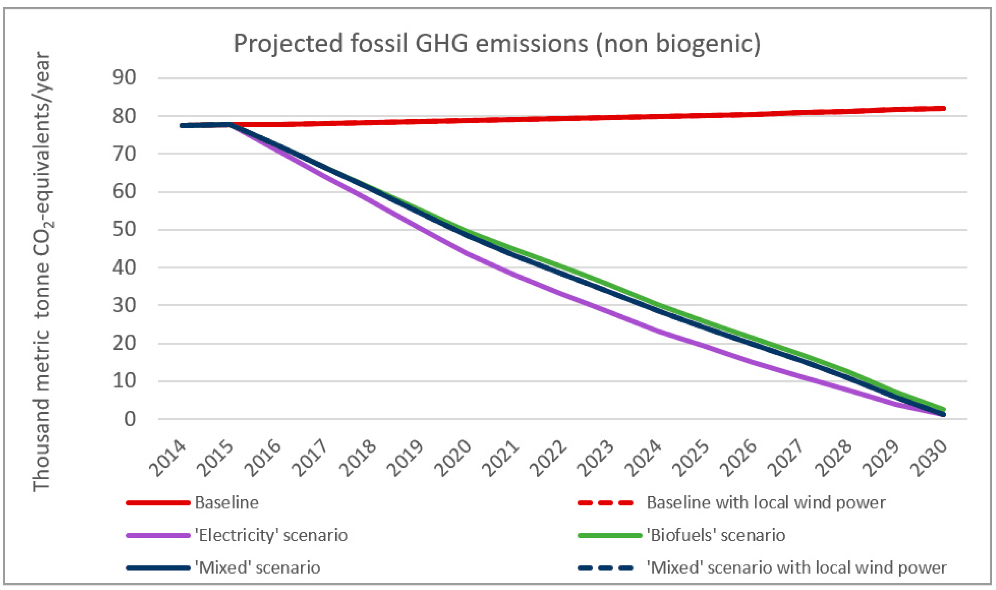
3.1. Impact of Local Climate Targets on Energy, Water and Land Use

The zero emissions target for the considered energy system is (as designed) reached by the year 2030 in the fossil-free scenarios ‘biofuels’, ‘electricity’ and ‘mix’, while emission levels in the baseline scenario (with and without local wind power exploitation) remain close to current levels. (Figure A2, Appendix B). All scenarios meet the same final energy service demands. However, as different scenarios take different routes to decarbonise, total primary energy requirements diverge over time (Figure 3a). Additionally, projected indirect future impacts on water and land use vary greatly (Figure 3b–d).
In the ‘biofuels’ and ‘mixed’ scenarios, the impacts from energy use on water consumption (Figure 3b) increase to more than four times the baseline values in 2030 despite an overall decline in primary energy demand (Figure 3a). The ‘electricity’ scenario initially follows this growing trend, but returns toward baseline values by 2030; this pattern is explained by the shift away from (first) the use of fossil fuels and (later) from biofuels in this scenario. Land use impacts (Figure 3c) follows the same pattern as water consumption, but with smaller divergence between scenarios over the modelled time horizon (the biofuels and mixed scenarios increase to between 2.5 and 3 times the baseline values in year 2030). In scenarios with local wind power, however, impacts on total land use increase much more (impacting approximately 3500 hectares more land than the same scenarios without wind power by the year 2030).
Regarding water withdrawal, the ‘electricity’ scenario has the biggest impact because thermal and hydroelectric power plants have highly demanding processes in terms of water withdrawal. For the same reason, scenarios ‘with local wind power’ show a sharp decrease in water withdrawal over the modelling period (since wind power is considered to require negligible amounts of water for its operation) [79].

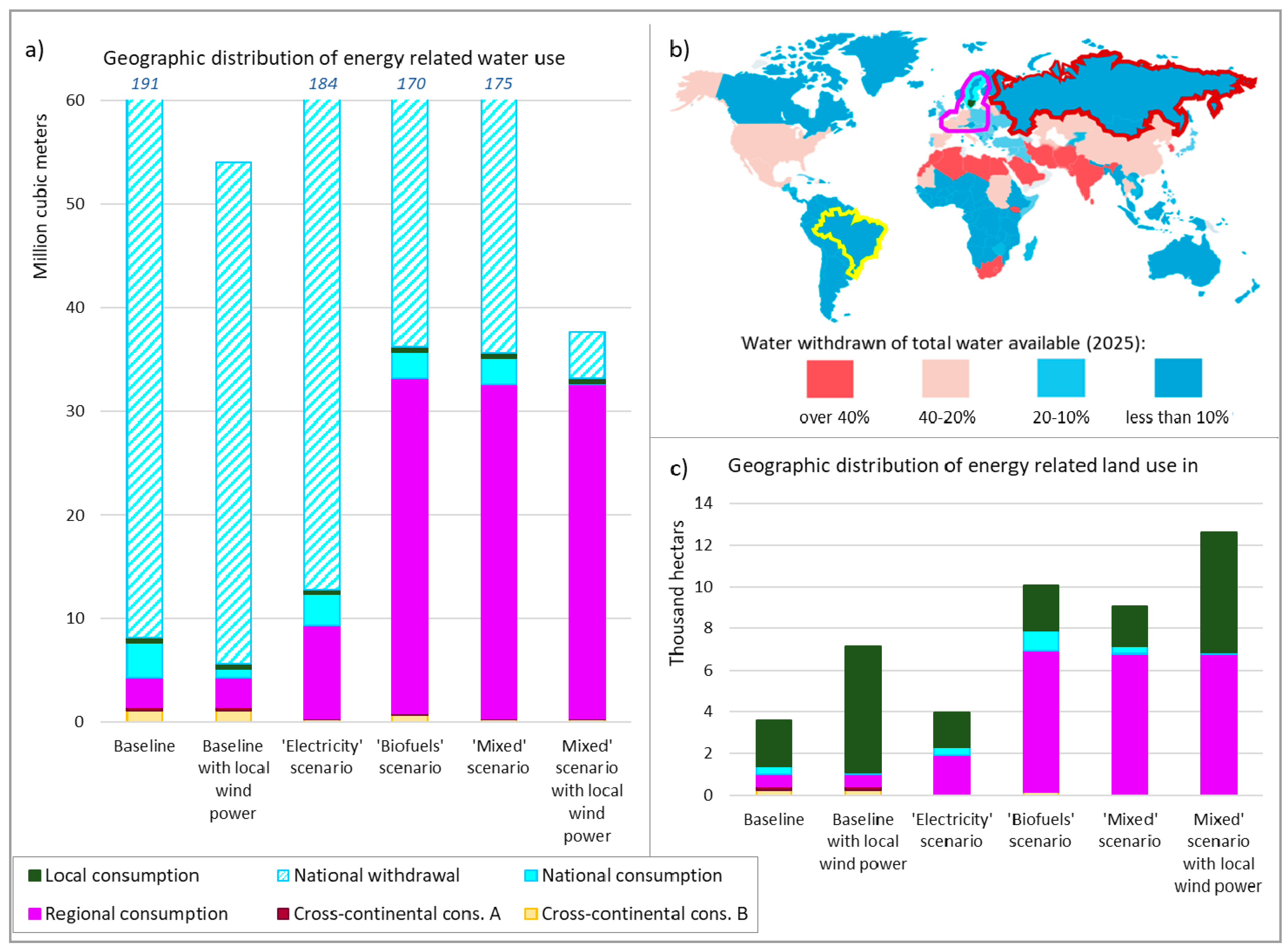
3.2. Geographical Distribution of Energy-Related Impacts on Water and Land Use

Figure 4a shows the distribution of projected water use for the year 2030 (in terms of both consumption and withdrawal) over geographic origin, for all scenarios. The distinction between water withdrawal and water consumption is only reported/applied for electricity generation (as mentioned in Section 2.2.2). For this reason, only electricity related water impacts (in Figure 4a corresponding to national water use) show different results between water consumption and withdrawal. Apart from the scenarios with local wind power, total water use (numbers above the total bars in Figure 4a) does not greatly differ among the scenarios. There is, however, considerably higher regional (here corresponding to European) water consumption (and somewhat smaller national water consumption and withdrawal) in the ‘biofuel’ and ‘mixed’ scenarios (without local wind) than in the ‘electricity’ and baseline scenarios (without local wind). This is primarily due to the use of imported biodiesel in the local transportation system in the ‘biofuel’ and ‘mixed’ scenarios. For these scenarios, the results indicate that a large share of the energy related water use is effectively ‘exported’ from Sweden to other parts of Europe.
Water stress, defined as the ratio of total withdrawn freshwater over the total available renewable freshwater resources in a region, is one of the key indicators for SDG6 [1]. The geographical distribution of energy-related water impacts (and in particular water withdrawals) should thus be assessed in relation to location-specific water availability. Figure 4b displays a world map of projected global water stress in 2025, with the geographies from Figure 4a indicated as highlighted borders. Overall, water availability within these impact boarders is projected to remain relatively abundant, except for regional water use within the bright pink border in Figure 4b. In the coming decades, biodiesel demands will need to be met at least partly by imports from some relatively water stressed European areas. As a consequence, scenarios with rapidly growing biodiesel shares (‘biofuels’ and ‘mixed’ scenarios) may then be constrained by (or contribute to) reduced water availability in such parts of Europe.
For land use (Figure 4c), regional and global impacts follow the same general pattern as that of regional and global water use: scenarios with dominant use of liquid biofuels (‘biofuels’ and ‘mixed’) require considerably more land use outside of Sweden. Locally, however, the pattern differs from that of water. Increased use of wind power and biomass-based heat and electricity have considerable local land use impacts. In scenarios with local wind power, the requirements of local land use double compared to corresponding scenarios without local wind power.

3.3. Sensitivity and Scalability of Local Case Results

3.3.1. Sensitivity Analysis for Cross-Resource Factors

Inherent uncertainties in both current and future interactions among different resource systems may change result aspects and implications. For gaining insight into the effects of such uncertainties, cross-resource input data values are analytically propagated through the local case model. For water consumption results, the most extreme input data generate outputs that are up to 150 times larger/smaller than those shown in Figure 3b and Figure 4a. When only considering input data values in the range between the 25th and 75th quantiles, this still gives up to 19 times larger/smaller results (see Appendix B, Figure A3).
Analogous uncertainty propagation is also carried out for the data on land use. Extreme output results are, in this case, between 5 and 15 times larger than the land use results in Figure 3c and Figure 4c (see Appendix B, Figure A3). For several of the investigated fuels, literature is found that reports land use impacts to be negligible. Specifically, local biofuels can be produced from waste or bi-products of other products [87], and might then have no ‘added’ impact on land use (however, a target of the SDG on sustainable production and consumption (SDG12) is to halve per capita food waste by 2030 [1].—hence, relying heavily on such waste resources for fuel production could become problematic). The lower extremes in the land use sensitivity ranges are for this reason close to zero for all scenarios.

3.3.2. Scaling to National Energy End Uses

The indirect water use—withdrawn and consumed—related to final energy use is lastly compared between the local case example (Oskarshamn) and the corresponding national case (Sweden) for the year 2010 (see Figure A4, Figure A5 and Figure A6). In that year, Sweden used 22% more energy per capita than Oskarshamn. The national energy mix included coal and natural gas (11% of total fuel end use), while Oskarshamn did not use these fuels. The country as a whole also used a larger share of liquid biofuels (11% vs. 1.3% of the corresponding total final fuel use). When these differences in energy use are translated to (energy related) water use, the Swedish average per-capita water consumption is more than 2.5 times larger than the Oskarshamn consumption. This is primarily due to the larger share of biofuels in the national energy mix. When looking at (energy related) water withdrawal, the Swedish average per capita withdrawal is only 11% higher than that of Oskarshamn. This smaller relative difference in per-capita water withdrawal compared to per-capita energy use (22%) is due to an only modest difference in per-capita electricity use (the main driver of water withdrawal impacts) between the local and the national case.

4. Discussion

4.1. Cross-Resource and Cross-Scale Implications

The aggregated results of the modelled scenarios (Figure 3) show that decarbonisation pathways diverge in terms of their various resource uses. Although primary energy use decreases in all fossil free scenarios (thanks to energy efficiency measures) (Figure 3a), both water consumption (Figure 3b) and land use (Figure 3c) increase. Water withdrawal patterns are less clear (Figure 3c). However, no single scenario is optimal (here corresponding to most resource efficient.) from all resource-use perspectives. Some use more land, some more water, and water use profiles vary greatly depending on whether focus lies on water withdrawal (which may limit water availability for energy use) or water consumption (which limits water availability for use in other sectors and for ecosystems). These results, albeit based on stylised scenarios, indicate that trade-offs are inevitable if local climate mitigation planning is to consider both land and water resources—and do so both locally and remotely. Still, such planning and policy are needed. To support local policy-making in weighing alternative impacts and minimise trade-offs, scenario analyses such as the one presented here could be valuable.
The presented results have implications beyond the studied municipality. In our simple local to national scaling, we find that Oskarshamn is not any extreme case compared to the national conditions. Rather, Oskarshamn may be viewed as slightly ‘better’ than the average Swedish situation: it uses less energy, less fossil fuels and less water-intensive liquid biofuels per capita than the average per-capita use in Sweden. The cross-resource and cross-scale implications of the local scale analysis hence cannot be discarded as some outlier community condition. As such, the identified implications provide important insights on cross-resource and cross-scale impacts of ambitious energy transitions and climate mitigation measures that may be implemented in many similar localities.

4.2. SDG Relations and Interactions

Relating the presented results to various SDGs, all scenarios are, as expected, positive towards the achievement of SDG7 (on clean energy), particularly targets 7.2 (increased shares of renewable energy) and 7.3 (doubling the global rate of improvement in energy efficiency). Furthermore, all fossil free scenarios are, by design, supporting SDG13 (climate action) and SDG11 (especially relating to its’ elements on urban climate mitigation) (As mentioned in Section 2.1, the local climate policy that constitutes the starting point of this analysis is devised by Oskarshamn as signatory of the Covenant of Mayors. In the Covenant of Mayor ‘commitment document’ SDG7, SDG11 and SDG13 are explicitly mentioned as international goals “to be considered” [88].) However, regarding cross-resource impacts, achievements towards SDG6 (for water), SDG15 (for life on land), SDG2 (for zero hunger), are affected differently (negatively or positively) in different decarbonisation scenarios. In Table 3, result implications for directly water and land related SDG targets (and indicators) of each decarbonisation scenario are assessed in a simple synergies/trade-offs categorisation.
Table 3 translates modelled scenario results for energy-related water and land uses to implications toward possible water- and land-related SDG achievement. Real consequences for SDG achievement are going to be more complicated, as exemplified in the following.
Assuming, for example, the quantity and geographic distribution of water withdrawn or consumed to remain constant for every unit of fuel used, our results indicate that future imports of water-intensive fuels will, at worst, come from moderately water stressed regions (Figure 4b). However, if future energy imports instead originate from more water stressed areas, a decarbonisation pathway that requires major water withdrawals would be more problematic from an SDG6 perspective. To give an illustrative example, ethanol from sugarcane grown in India could, in the extreme case, be up to 40 times more water intensive compared to Brazilian sugarcane-based ethanol [89]. India is projected to be highly water stressed by year 2025 (Figure 4b). Ethanol imports to Oskarshamn are not anticipated to increase in the coming decades, nor is the origin of the fuel expected to shift towards India. However, in the hypothetical case of this happening, such water stress could jeopardise the security of supply to Oskarshamn (if water is not available for fuel production). Further, if a large number of Covenant of Mayor’s signatories (such as Oskarshamn) would promote (Indian) ethanol to replace fossil transportation fuels this could potentially exacerbate the water stress in India (since we assume that withdrawn water for biofuels is also consumed—and hence removed from the region).
Furthermore, although scenarios with local wind power show large increases in land use, wind power plants do not physically occupy more than a small share of the total required land area [90]. From a biodiversity—and SDG15—perspective, the large land use requirement for wind power may thus not be an issue of concern per se. Wind power may affect birds and bats considerably [91] and create fragmentation of the landscape [92], but do not completely change the land structure (and thereby the terrestrial eco-system) upon which they are placed. The large international impacts of biodiesel use on land use may be more problematic. In both Sweden and Germany, with projected cultivation of rapeseeds for biodiesel [36], land use requirements may come in more direct conflict with either food production (SDG2) or biodiversity conservation (SDG15). Hence, while both biodiesel and wind power can contribute to reaching SDG7 and SDG13, the former could have considerably larger negative impacts on the progress towards SDG2 and SDG15. Future studies need to further consider impact levels on land of different quality.
There are several additional interactions with and among these and other SDGs than the ones focused on here [93]. For example, the SDGs relating to energy, agriculture and water use have numerous interdependencies, globally, in different regions, and for different human sectors and activities [6,94]. By considering at least some of the SDGs and their interactions (synergies/trade-offs) in comparative scenario modelling, this study has taken a step beyond general mapping and shown essential development-pathway dependence. This type of investigation of cross-scale and cross-resource nexus impacts, specifically focusing on implications of the local on the “global” and on cross-SDG progress, has not been done previously with a CLEWs approach.

4.3. Uncertainty Implications

The reported data required for quantification of cross-resource interactions vary over large value ranges (Figure 2 and Appendix B, Figure A1). The results of this study are sensitive to this variation. Overall, scenarios with large shares of biofuels emerge as more impactful on both consumptive water use and land use. However, when exploring the sensitivity of these results to the full ranges of reported water and land use data, they lose in clarity and distinction (Appendix B, Figure A3). This is not surprising considering the large ranges reported for essential input data values, but stresses the importance of further investigation on how various resource uses are measured and reported. In particular, it emphasises the need for more accurate, location specific and standardised land and water use data across fuel groups (More and comparable data, consistently reported for all fuels, may not necessarily reduce uncertainties. However, they could allow more sophisticated uncertainty analysis with uncertainty quantification techniques such as Monte Carlo simulations or similar).
Nevertheless, even with these levels of uncertainty, the investigated scenarios (including the ‘baseline’) show some clear energy transformation impacts on water and land resources locally to globally. This study thereby highlights the importance to consider cross-resource, cross-scale and cross-SDG interactions in local energy decisions. Additionally, the results showcase the potential of the type of analysis presented here. Through this type of assessment, CLEW nexus-related resource and SDG interactions are traceable and quantifiable, and could—with improved data availability—provide policy- and decision-makers with important insights for progress on several SDGs.

5. Concluding Remarks

Strategies for moving towards achieving SDGs on climate action (SDG13), sustainable cities (SDG11) and clean energy (SDG7) are not just linked with each other, but also with other SDGs. This study highlights such interactions related to water (SDG6) and land use (SDG15, SDG2) for a local Swedish case example. It shows that such interactions vary in intensity and geography depending on chosen local decarbonisation strategy. Hence, these SDG interactions and their geographic distribution are highly path-dependent.
Due to large variations in reported values of required data for studying cross-resource interactions, the numerical results of this study are indicative. Still, they clearly show that local decision-makers, such as those in Oskarshamn, have power to influence parts of the world far outside their local jurisdiction. Insights from thought experiments like those in this study—including its sensitivity analysis—may be critically important for understanding the broader resource impacts of local decisions (complemented by efforts to seek more and better data).
To support relevant extensions of the modelling framework presented here, we call for common data collection approaches with transparent methodologies (including their uncertainties) to improve the comparability of resource use data across the energy system. Such data improvements are imperative for improving the accuracy of system wide analyses such as the one presented here. This is also needed to move beyond the indicative and enable analysis that can feed realistic numerical results into policy dialogue on the specificities of SDG interactions.
This study highlights how ambitious local level policy aimed at climate mitigation may impact resource use elsewhere. Still, ambitious policymaking is needed to meet international commitments on climate change—and local actions is crucial. However, for global progress to be made towards all SDGs, such local actions need to be carried out with sensitivity towards that a local optimum is not necessarily the global optimum.

Supplementary Materials

The following are available online at https://www.mdpi.com/2071-1050/11/7/1847/s1: LEAP file of the Oskarshamn energy system model including all analysed scenarios.

Author Contributions

The authors of this paper has contributed to the work as follows: conceptualization, R.E., G.D., M.H., H.R. and M.B.; methodology, R.E. and M.H.; software, R.E., M.H. and V.R.; validation, R.E., G.D. and M.H.; formal analysis, R.E.; investigation, R.E.; data curation, R.E. and V.R.; writing—original draft preparation, R.E.; writing—review and editing, R.E., G.D., M.H., H.R. and M.B.; visualization, R.E.; supervision, G.D. and M.H.; project administration, R.E.; funding acquisition, G.D. and M.H.

Funding

This research was funded by the Swedish Research Council Formas (grant numbers 2016-02045 (R.E., G.D.) and 2015-1304 (R.E., M.H.)).

Acknowledgments

The authors would like to gratefully acknowledge the support and assistance in data collection by Katarina Skoglycka at Oskarshamns kommun, Bengt Karlsson at Nova Utbildning FoU & Affärsutveckling in Oskarshamn; and Per-Ola Bergström at Oskarshamn Energi.

Conflicts of Interest

The authors declare no conflict of interest. The funders had no role in the design of the study; in the collection, analyses, or interpretation of data; in the writing of the manuscript, or in the decision to publish the results.

Appendix A. Model Design and Assumptions

The LEAP energy model developed for this study simulates the energy system of Oskarshamn municipality between the years 2012 and 2040 (with results analysed for the years 2014–2030). Given the objective of the study—to assess potential water and land use impacts of local pathways to rapid decarbonisation—the model is set up as an illustrative case of a local system. As such, it is only in the baseline scenario that current local trends in energy supply are extrapolated. All fossil free scenarios follow population and GDP growth projections, and the related demands for energy services. However, they move away from following historic trends on the supply side of the energy system, since extrapolating those trends do not phase out fossil fuels.
The transition away from fossil fuels within such a short period (16 years) leads in some cases to brutal/dramatic shifts in supply chains. The present study does not claim that these shifts are the most probable. It is likely that the future contains technological and societal innovations that are not anticipated here. However, for the purpose of illustrating what a local goal to decarbonise could require of the energy system (and the water and land systems that the energy system is dependent on), a few extreme assumptions are kept in the model.
In the following, key modelling data and assumptions are listed.

Appendix A.1. Final Energy (Service) Demands

Projected changes in population [73] and household size [70] determine residential energy demands. Population change also drive passenger transport needs and determine the availability of municipal solid waste and wastewater (as potential feed stock for biogas production). Projected GDP growth drives total demands for energy in the commercial and industrial sectors and determine the freight transport demands. Agricultural energy demands are estimated based on projected total land use for agriculture [74].

Appendix A.2. Energy Efficiency, Supply Technologies, and Fuel Availability

While energy service demands are modelled based on the above trends, possible ways to meet those demands in the future are many. Significant energy efficiency improvements are modelled in all fossil free scenarios within the end use sectors—residential, commercial, industry, transport and agriculture. Further, technology shifts, including fuel shifts are modelled in all sectors. Table A1, Table A2, Table A3 and Table A4 below detail these modelled changes in the energy system compared to the baseline scenario.
Table A1. Energy efficiency assumptions.
Efficiency MeasureEfficiency Improvement by 2030 Compared to BaselineReference
Residential and commercial electrical appliances50%[95]
Residential cooking energy intensity20%[96]
Residential and commercial lighting85%[70]
Residential and commercial building insulation—impacting total heating demand by…20%[70]
Street light energy intensity50% [97]
Energy intensity of industry38% [76] finds potential to reduce by 40% compared to present level. Since the baseline energy intensity increases, this is a more conservative assumption.
Freight transport within the municipality 10% reduction in vehicle-kilometres travelled by freight transportsThis is a modest estimate by the authors based on unquantified ambitions to decrease the number of vehicle-kilometres travelled [51].
Table A2. Technology/fuel switching assumptions outside buildings (Table A3) and personal transport (Table A4) sectors.
Energy System ComponentTechnology/Fuel SwitchReference
Industrial process heatFossil oil is replaced with (>80% biomass based) district heat and electricity (district heating assumed to be feasible up to 89% (modelled in the biofuels scenario). In the electricity scenario, electricity and district heating cover 50% each of the replaced oil heating demand.Based on the patterns suggested by [76]
Freight transport and agricultural sector All use of fossil diesel is replaced by biodiesel (pure FAME)According to [98] the use of pure FAME based on RME is increasing.
Table A3. Share of space and water heating technologies in 2030 considered in baseline and fossil free scenarios.
Space Heating Technology Baseline Scenario‘Electricity’ Scenario‘Biofuels’ + ‘Mixed’ Scenarios
Detached houses% shares in 2030% shares in 2030% shares in 2030
-
Heat Pump
50.66565
-
District heating
3.644
-
Pellets fired
452323
-
Oil fired
0.800
-
Solar heat
088
Apartments
-
Heat Pump
15.81612
-
District heating
848084
-
Oil fired
0.200
-
Solar heat
044
Commercial buildings
-
Heat Pump
587658
-
District heating
202038
-
Oil fired
2200
-
Solar heat
044
Table A4. Vehicle fleet in Oskarshamn in 2012, and in 2030 for the baseline and fossil free scenarios.
Vehicle Fleet in Year…20122030 in Each Scenario:
BaselineElectricity and MixedBiofuels
Personal Vehicles (no. of vehicles)Diesel22627130233 *1094 *
Gasoline109254942310310
Plug in electric619410681463
Biogas341504446216
Ethanol65323405371468
Electric14109863027
Total13936146601357713577
Public transport (no. of buses)Diesel202000
Biogas00737
Plug in electric00355
Total20204242
* Assumed to be fuelled with biodiesel by 2030.
In addition to the above shift between personal vehicles and from personal vehicles to public transport, 4% of total number of vehicles are removed in the fossil free scenarios without replacement by buses or other vehicles, assumed to be replaced by increased walking and biking. Oskarshamn specifically mentions, without quantifying, that the municipality will increase efforts to facilitate biking and walking for its citizens [51]. This decrease in total road vehicles is therefore likely an underestimate.

Appendix A.3. Water and Land-Use Impacts

Water and land-use data are converted to comparable units (m3/TJ and hectare/TJ respectively) for each energy carrier in the Oskarshamn energy system. See Figure 2 (main manuscript) and Figure A2 for full ranges of data considered. Table A5 shows selected data points used to model the Oskarshamn energy system, with reference and geographical origin of data included.
Table A5. Water and land use factors used for the Oskarshamn energy model, including references and the geographical origin of the data.
FuelGeographic Origin (of Fuel)Consumptive Water Use (m3/TJ)Geographic Origin of ReferenceReferenceLand Use (ha/TJ)Geographic Origin of ReferenceReference
Crude oil—refined to heating oil, gasoline and dieselRussia133SpainCalculated based on data from [79,99]0.1266CanadaCalculated based on reported data from [82].
Electricity (incl. (nuclear) fuel extraction)Sweden (Canada)2222RussiaCalculated from electricity generation factors per source fuel and the Swedish electricity mix.
-
Data comes from [100], corresponding to Russian hydropower plant. (3600 m3/TJ)
-
Nuclear power generation water use is taken from [80]. Power plant cooling water is not included since this is made up of seawater in Sweden [101]. (86 m3/TJ)
-
Other thermal power plant water use are calculated based on [99,102,103]
0.266Nordic (Canada)Calculated from electricity generation factors per source fuel [37,53,104] and the Swedish electricity mix [61].
Wind powerOskarshamn0USA / GlobalAssumed negligible by [79,105].3.47Oskarshamn[53]
Biogas (if imported)Oskarshamn (Sweden)0 (454)ItalyLocally produced biogas is assumed to come from sewage sludge, manure and similar wet waste products (requiring no added water). Imported biogas may come from dry matter, therefore requiring water in the anaerobic process as assumed by [27]0 (5.6)EU[36]
Biomass (from forest residues)Oskarshamn612USA[106]2.5Spain[107], assuming forest residues to “occupy” 5% of the land they are harvested from
Biomass (from Grass) Oskarshamn0SwedenBased on description in [108]8.4OskarshamnSwedish Biogas International AB (2008), assuming that the crop ”occupy” 70% of the land it is harvested from (assumption based on data patterns in [36].
Ethanol from sugar caneBrazil24695“Global average”[81]5.0Latin America [36]
Biodiesel from rapeseedEU (Sweden and Germany)57047USA[79]11.9EU[36]
Notes to Table A5:
  • Solid biofuels (biomass) are included in the Oskarshamn energy model in two formats: forest based pellets or wood fuel for residential heating and district heating, and grassy biomass for biogas production (in conjunction with manure and municipal sewage) and for district heating. It is assumed that the grassy biomass is inserted in the energy system without pre-processing, thereby requiring no additional water. Further, the grass is expected to grow without irrigation. Conversion of forest biomass to pellets are considered to require some water.
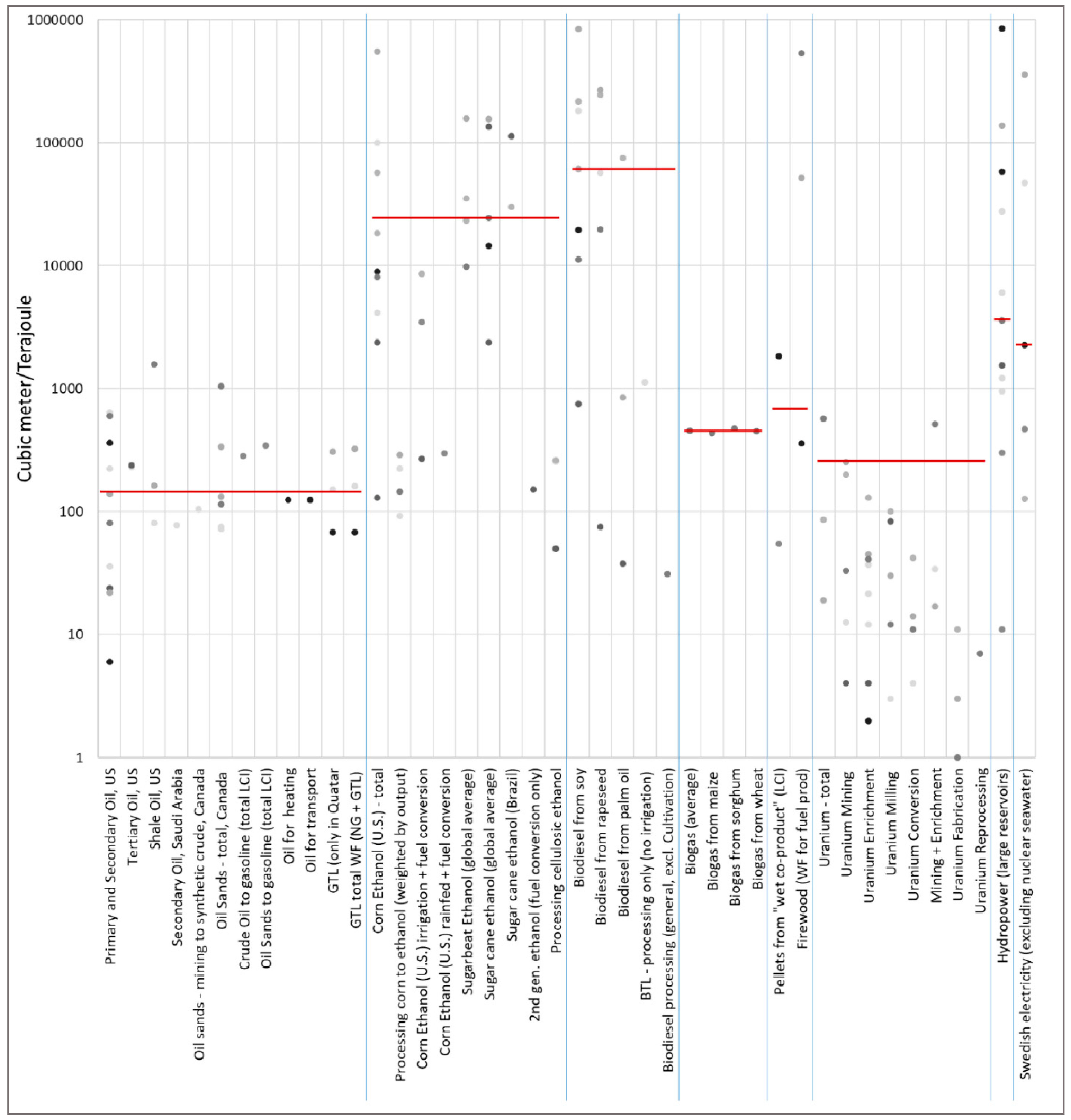
  • As highlighted in the main manuscript all data describing cross-resource interaction between water, land and energy are reported in large ranges. Data points selected to describe these relationships in the model are therefore to be interpreted as reasonable guesses rather than exact representations of the real interactions. See further discussion on sensitivity of results and need for further developments in data collection and modelling approaches in main manuscript.

Appendix A.3.1. References of Data Sources Reviewed for Energy Related Water Use and Land Use

The below references have been reviewed for collecting data on energy related water consumption. These data are displayed in Figure 2:
  • Pacetti, T., Lombardi, L. & Federici, G. Water-energy Nexus: a case of biogas production from energy crops evaluated by Water Footprint and Life Cycle Assessment (LCA). J. Clean. Prod. 101, 278–291 (2015).
  • Mekonnen, M. M., Gerbens-Leenes, P. W. & Hoekstra, A. Y. The consumptive water footprint of electricity and heat: a global assessment. Environ. Sci. Water Res. Technol. 1, 285–297 (2015).
  • Levi, L., Jaramillo, F., Andricevic, R. & Destouni, G. Hydroclimatic changes and drivers in the Sava River Catchment and comparison with Swedish catchments. Ambio 44, 624–634 (2015).
  • Spang, E. S., Moomaw, W. R., Gallagher, K. S., Kirshen, P. H. & Marks, D. H. The water consumption of energy production: an international comparison. Environ. Res. Lett. 9, 105002 (2014).
  • International Energy Agency. World Energy Outlook 2012. (OECD/IEA, 2012).
  • Macknick, J., Newmark, R., Heath, G. & Hallett, K. C. Operational water consumption and withdrawal factors for electricity generating technologies: a review of existing literature. Environ. Res. Lett. 7, 045802 (2012).
  • Herath, I., Deurer, M., Horne, D., Singh, R. & Clothier, B. The water footprint of hydroelectricity: a methodological comparison from a case study in New Zealand. J. Clean. Prod. 19, 1582–1589 (2011).
  • Scown, C. D., Horvath, A. & McKone, T. E. Water Footprint of U.S. Transportation Fuels. Environ. Sci. Technol. 45, 2541–2553 (2011).
  • Katers, J. F. & Snippen, A. Life-cycle Inventory of Wood Pellet Manufacturing in Wisconsin. 43 (Public Service Commission of Wisconsin & the Statewide Energy Efficiency and Renewables Administration, 2011).
  • Granit, J. & Lindström, A. Constraints and opportunities in meeting the increasing use of water for energy production. in Proceedings of the ESF Strategic Workshop on: Accounting for water scarcity and pollution in the rules of international trade 54, (UNESCO-IHE Institute for Water Education, 2010).
  • Mielke, E., Anadon, L. D. & Narayanamurti, V. Water consumption of energy resource extraction, processing, and conversion. (Belfer Center for Science and International Affairs, Harvard Kennedy School, Harvard University, 2010).
  • Fthenakis, V. & Kim, H. C. Life-cycle uses of water in U.S. electricity generation. Renew. Sustain. Energy Rev. 14, 2039–2048 (2010).
  • Rio Carrillo, A. M. & Frei, C. Water: A key resource in energy production. Energy Policy 37, 4303–4312 (2009).
  • Gerbens-Leenes, W. & Hoekstra, A. Y. The water footprint of sweeteners and bio-ethanol from sugar cane, sugar beet and maize. (2009).
  • Gerbens-Leenes, P. W., Hoekstra, A. Y. & Meer, T. H. Water footprint of bio-energy and other primary energy carriers. (UNESCO-IHE Institute for Water Education, 2008).
  • Union of Concerned Scientists. UCS EW3 Energy-Water Database V.1.3. (2012).
  • Swedenenergy. Fjärrvärmestatistik—Energiföretagen Sverige. (2015). Available at: http://www.svenskfjarrvarme.se/Statistik--Pris/Fjarrvarme/Energitillforsel/. (Accessed: 11th December 2017)
  • Miljösamverkan Västra Götaland. Vägledning för miljötillsyn vid fjärrvärmeanläggningar. (2007).
The below references have been reviewed for collecting data on energy related land use. These data are displayed in Figure A1:
  • Vattenfall AB. Certified Environmental Product Declaration EPD® of Electricity from Vattenfall Nordic Nuclear Power Plants. (2016).
  • Vattenfall AB. Certified Environmental Product Declaration EPD® of Electricity from Vattenfall Nordic Wind Farms. (2016).
  • Vattenfall AB. Certified Environmental Product Declaration EPD® of Electricity from Vattenfall’s Nordic Hydropower. (2015).
  • Valin, H. et al. The land use change impact of biofuels consumed in the EU. Quantification of area and greenhouse gas impacts. (ECOFYS, 2015).
  • Energikontor Sydost & Biogas Sydost. Regional strategi och handlingsplan för biogas till fordon i Blekinge, Kalmar och Kronobergs län. Åtgärder 2014–2017 med utblick till 2020. Växjö (Energikontor Sydost AB, 2014).
  • Yeh, S. et al. Land Use Greenhouse Gas Emissions from Conventional Oil Production and Oil Sands. Environ. Sci. Technol. 44, 8766–8772 (2010).
  • Gómez, A., Rodrigues, M., Montañés, C., Dopazo, C. & Fueyo, N. The potential for electricity generation from crop and forestry residues in Spain. Biomass Bioenergy 34, 703–719 (2010).
  • Fthenakis, V. & Kim, H. C. Land use and electricity generation: A life-cycle analysis. Renew. Sustain. Energy Rev. 13, 1465–1474 (2009).
  • Denholm, P. & Margolis, R. M. Land-use requirements and the per-capita solar footprint for photovoltaic generation in the United States. Energy Policy 36, 3531–3543 (2008).
  • Swedish Biogas International. Möjligheter för biogas i Kalmar län-en idéstudie. 88 (Swedish Biogas International, 2008).

Appendix B. Supplementary Figures

Figure A1 shows the range of land use data considered for each fuel for this study.
Figure A1. Energy-related land use data reported in different literature sources. Data sources listed in Appendix A.3.1.
Sustainability 11 01847 g0a1
Note to Figure A1:
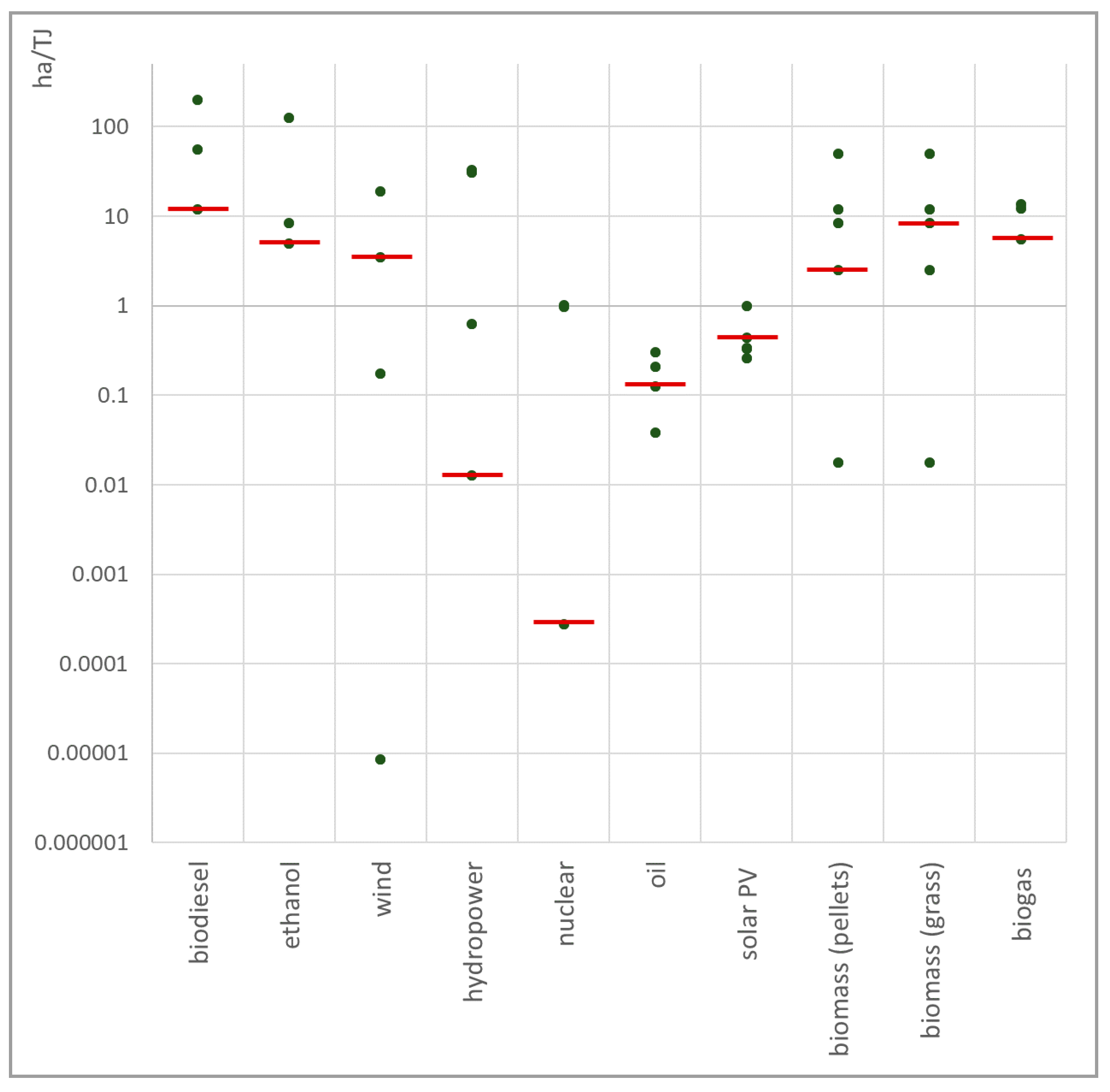
  • Nuclear energy land use requirements are not including estimated land use needs for final repository of used fuel. It is therefore anticipated that the total land area excluded from other uses due to nuclear energy is larger than reported here.
Figure A2 shows the modelled results on non-biogenic CO2 emissions in the Oskarshamn energy system for studied scenarios.
Figure A2. Modelled impacts on GHG emissions, in CO2-equivalents, from all local scenarios assessed.
Sustainability 11 01847 g0a2
Figure A3 displays result ranges of total energy related water consumption and land use when exposed to uncertainty in input data. Input data are here only varied for water consumption factors and land use factors across the full range of reviewed data. These input data ranges are displayed in Figure 2 in main manuscript and Figure A1 above.
Figure A3. Output sensitivity plots for water consumption (LHS) and land use (RHS) requirements of each scenario in model year 2030. Boxed values are varied between Q1 and Q3. Stars marks the results presented in the main manuscript (Figure 3 and Figure 4). Whiskers cover result sensitivity between maximum and minimum input data values.
Sustainability 11 01847 g0a3
Figure A4, Figure A5 and Figure A6 show the results of the comparisons of energy use related water impacts between the nation of Sweden and the municipality of Oskarshamn.
Figure A4. Total final energy use in Oskarshamn and in Sweden in year 2010 (data from [83]).
Sustainability 11 01847 g0a4
Figure A5. Calculated impacts on water consumption and water withdrawal in Sweden and Oskarshamn from the energy use presented in Figure A4 distributed over fuel groups.
Sustainability 11 01847 g0a5
Figure A6. Calculated impacts on water consumption and water withdrawal in Sweden and Oskarshamn from the energy use presented in Figure A4 distributed over energy use sectors.
Sustainability 11 01847 g0a6

References

  1. UN General Assembly. Transforming Our World: The 2030 Agenda for Sustainable Development; United Nations: New York, NY, USA, 2015. [Google Scholar]
  2. Griggs, D.; Nilsson, M.; Stevance, A.; McCollum, D. A Guide to SDG Interactions: From Science to Implementation; International Council for Science (ICSU): Paris, France, 2017. [Google Scholar]
  3. International Energy Agency (IEA) & the World Bank. Sustainable Energy for All 2015—Progress toward Sustainable Energy 2015; World Bank: Washington, DC, USA, 2015. [Google Scholar] [CrossRef]
  4. Nilsson, M.; Griggs, D.; Visbeck, M. Policy: Map the interactions between Sustainable Development Goals. Nat. News 2016, 534, 320. [Google Scholar] [CrossRef]
  5. Nerini, F.F.; Tomei, J.; To, L.S.; Bisaga, I.; Parikh, P.; Black, M.; Borrion, A.; Spataru, C.; Broto, V.C.; Anandarajah, G. Mapping synergies and trade-offs between energy and the Sustainable Development Goals. Nat. Energy 2018, 3, 10–15. [Google Scholar] [CrossRef]
  6. Pradhan, P.; Costa, L.; Rybski, D.; Lucht, W.; Kropp, J.P. A Systematic Study of Sustainable Development Goal (SDG) Interactions. Earths Future 2017, 5, 1169–1179. [Google Scholar] [CrossRef] [Green Version]
  7. Covenant of Mayors. Available online: http://www.covenantofmayors.eu/index_en.html (accessed on 28 March 2017).
  8. Bulkeley, H.; Castán Broto, V.; Edwards, G. Bringing climate change to the city: Towards low carbon urbanism? Local Environ. Int. J. Justice Sustain. 2012, 17, 545–551. [Google Scholar] [CrossRef]
  9. Rosenzweig, C.; Solecki, W.; Hammer, S.A.; Mehrotra, S. Cities lead the way in climate-change action. Nature 2010, 467, 909–911. [Google Scholar] [CrossRef]
  10. Acuto, M. City Leadership in Global Governance. Glob. Gov. Rev. Multilater. Int. Organ. 2013, 19, 481–498. [Google Scholar] [CrossRef]
  11. Hussey, K.; Pittock, J. The Energy–Water Nexus: Managing the Links between Energy and Water for a Sustainable Future. Ecol. Soc. 2012, 17. [Google Scholar] [CrossRef] [Green Version]
  12. Engström, R.E.; Howells, M.; Destouni, G. Water impacts and water-climate goal conflicts of local energy choices—Notes from a Swedish perspective. Proc. IAHS 2018, 376, 25–33. [Google Scholar] [CrossRef]
  13. Pincetl, S. Nature, urban development and sustainability—What new elements are needed for a more comprehensive understanding? Cities 2012, 29 (Suppl. 2), S32–S37. [Google Scholar] [CrossRef]
  14. Bazilian, M.; Rogner, H.; Howells, M.; Hermann, S.; Arent, D.; Gielen, D.; Steduto, P.; Mueller, A.; Komor, P.; Tol, R.S.; et al. Considering the energy, water and food nexus: Towards an integrated modelling approach. Energy Policy 2011, 39, 7896–7906. [Google Scholar] [CrossRef]
  15. De Strasser, L.; Lipponen, A.; Howells, M.; Stec, S.; Bréthaut, C. A methodology to assess the water energy food ecosystems nexus in transboundary river basins. Water 2016, 8, 59. [Google Scholar] [CrossRef]
  16. Howells, M.; Hermann, S.; Welsch, M.; Bazilian, M.; Segerström, R.; Alfstad, T.; Gielen, D.; Rogner, H.; Fischer, G.; Van Velthuizen, H.; et al. Integrated analysis of climate change, land-use, energy and water strategies. Nat. Clim. Chang. 2013, 3, 621–626. [Google Scholar] [CrossRef]
  17. Macknick, J.; Sattler, S.; Averyt, K.; Clemmer, S.; Rogers, J. The water implications of generating electricity: Water use across the United States based on different electricity pathways through 2050. Environ. Res. Lett. 2012, 7, 045803. [Google Scholar] [CrossRef]
  18. Märker, C.; Venghaus, S.; Hake, J.-F. Integrated governance for the food–energy–water nexus—The scope of action for institutional change. Renew. Sustain. Energy Rev. 2018, 97, 290–300. [Google Scholar] [CrossRef]
  19. Smajgl, A.; Ward, J. The Water-Food-Energy Nexus in the Mekong Region: Assessing Development Strategies Considering Cross-Sectoral and Transboundary Impacts; Springer Science & Business Media: New York, NY, USA, 2013. [Google Scholar]
  20. United Nations. Prototype Global Sustainable Development Report; United Nations Department of Economic and Social Affairs, Division for Sustainable Development: New York, NY, USA, 2014. [Google Scholar]
  21. Destouni, G.; Jaramillo, F.; Prieto, C. Hydroclimatic shifts driven by human water use for food and energy production. Nat. Clim. Chang. 2013, 3, 213–217. [Google Scholar] [CrossRef]
  22. Levi, L.; Jaramillo, F.; Andricevic, R.; Destouni, G. Hydroclimatic changes and drivers in the Sava River Catchment and comparison with Swedish catchments. Ambio 2015, 44, 624–634. [Google Scholar] [CrossRef] [Green Version]
  23. Jaramillo, F.; Destouni, G. Comment on “Planetary boundaries: Guiding human development on a changing planet”. Science 2015, 348, 1217. [Google Scholar] [CrossRef]
  24. Zhou, Y.; Zhang, B.; Wang, H.; Bi, J. Drops of energy: Conserving urban water to reduce greenhouse gas emissions. Environ. Sci. Technol. 2013, 47, 10753–10761. [Google Scholar] [CrossRef]
  25. International Energy Agency. WEO 2016 Special Report: Water Energy Nexus; International Energy Agency: Paris, France, 2017; 63p. [Google Scholar]
  26. Gerbens-Leenes, P.W.; Van Lienden, A.R.; Hoekstra, A.Y.; Van der Meer, T.H. Biofuel scenarios in a water perspective: The global blue and green water footprint of road transport in 2030. Glob. Environ. Chang. 2012, 22, 764–775. [Google Scholar] [CrossRef] [Green Version]
  27. Pacetti, T.; Lombardi, L.; Federici, G. Water–energy Nexus: A case of biogas production from energy crops evaluated by Water Footprint and Life Cycle Assessment (LCA) methods. J. Clean. Prod. 2015, 101, 278–291. [Google Scholar] [CrossRef]
  28. Scown, C.D.; Horvath, A.; McKone, T.E. Water Footprint of U.S. Transportation Fuels. Environ. Sci. Technol. 2011, 45, 2541–2553. [Google Scholar] [CrossRef]
  29. Macknick, J.; Newmark, R.; Heath, G.; Hallett, K.C. Operational water consumption and withdrawal factors for electricity generating technologies: A review of existing literature. Environ. Res. Lett. 2012, 7, 045802. [Google Scholar] [CrossRef]
  30. Mekonnen, M.M.; Gerbens-Leenes, P.W.; Hoekstra, A.Y. The consumptive water footprint of electricity and heat: A global assessment. Environ. Sci. Water Res. Technol. 2015, 1, 285–297. [Google Scholar] [CrossRef]
  31. Jaramillo, F.; Destouni, G. Local flow regulation and irrigation raise global human water consumption and footprint. Science 2015, 350, 1248–1251. [Google Scholar] [CrossRef]
  32. Cheng VK, M.; Hammond, G.P. Life-cycle energy densities and land-take requirements of various power generators: A UK perspective. J. Energy Inst. 2017, 90, 201–213. [Google Scholar] [CrossRef]
  33. Denholm, P.; Margolis, R.M. Land-use requirements and the per-capita solar footprint for photovoltaic generation in the United States. Energy Policy 2008, 36, 3531–3543. [Google Scholar] [CrossRef]
  34. Fthenakis, V.; Kim, H.C. Land use and electricity generation: A life-cycle analysis. Renew. Sustain. Energy Rev. 2009, 13, 1465–1474. [Google Scholar] [CrossRef] [Green Version]
  35. Hermann, S.; Welsch, M.; Segerstrom, R.E.; Howells, M.I.; Young, C.; Alfstad, T.; Rogner, H.H.; Steduto, P. Climate, land, energy and water (CLEW) interlinkages in Burkina Faso: An analysis of agricultural intensification and bioenergy production. Nat. Resour. Forum 2012, 36, 245–262. [Google Scholar] [CrossRef]
  36. Valin, H.; Peters, D.; van den Berg, M.; Frank, S.; Havlik, P.; Forsell, N.; Hamelinck, C.; Pirker, J.; Mosnier, A.; Balkovič, J.; et al. The Land Use Change Impact of Biofuels Consumed in the EU. Quantification of Area and Greenhouse Gas Impacts; Ecofys: Utrecht, The Netherlands, 2015. [Google Scholar]
  37. Vattenfall AB. Certified Environmental Product Declaration EPD® of Electricity from Vattenfall’s Nordic Hydropower, UNCPC Code 17, Group 171 - Electrical Energy. Vattenfall AB, 2015. Available online: https://www.environdec.com/Detail/?Epd=11982 (accessed on 12 March 2019).
  38. Liu, H.; Huang, Y.; Yuan, H.; Yin, X.; Wu, C. Life cycle assessment of biofuels in China: Status and challenges. Renew. Sustain. Energy Rev. 2018, 97, 301–322. [Google Scholar] [CrossRef]
  39. Singlitico, A.; Goggins, J.; Monaghan, R.F.D. The role of life cycle assessment in the sustainable transition to a decarbonised gas network through green gas production. Renew. Sustain. Energy Rev. 2019, 99, 16–28. [Google Scholar] [CrossRef]
  40. Uctug, F.G.; Azapagic, A. Environmental impacts of small-scale hybrid energy systems: Coupling solar photovoltaics and lithium-ion batteries. Sci. Total Environ. 2018, 643, 1579–1589. [Google Scholar] [CrossRef]
  41. Pioletti, M.; Brigolin, D.; Pastres, R. The life cycle impact of energy final uses in small urban systems: Implications for emission accounting and EU sustainable local energy planning. Sustain. Cities Soc. 2018, 42, 252–258. [Google Scholar] [CrossRef]
  42. Holland, R.A.; Scott, K.A.; Flörke, M.; Brown, G.; Ewers, R.M.; Farmer, E.; Kapos, V.; Muggeridge, A.; Scharlemann, J.P.; Taylor, G.; et al. Global impacts of energy demand on the freshwater resources of nations. Proc. Natl. Acad. Sci. USA 2015, 112, E6707–E6716. [Google Scholar] [CrossRef] [Green Version]
  43. Howard, D.C.; Wadsworth, R.A.; Whitaker, J.W.; Hughes, N.; Bunce, R.G.H. The impact of sustainable energy production on land use in Britain through to 2050. Land Use Policy 2009, 26, S284–S292. [Google Scholar] [CrossRef]
  44. C40 & Ramboll. Urban Climate Action Impact Framework. A Framework for Describing and Measuring the Wider Impacts of Urban Climate Action; C40: London, UK, 2018. [Google Scholar]
  45. Sachs, J.; Schmidt-Traub, G.; Kroll, C.; Durand-Delacre, D.; Teksoz, K. SDG Index and Dashboards Report 2017; Bertelsmann Stiftung and Sustainable Development Solutions Network (SDSN): New York, NY, USA, 2017. [Google Scholar]
  46. Sachs, J.; Schmidt-Traub, G.; Kroll, C.; Lafortune, G.; Fuller, G. SDG Index and Dashboards Report 2018; Bertelsmann Stiftung and Sustainable Development Solutions Network (SDSN): New York, NY, USA, 2018. [Google Scholar]
  47. Sachs, J.; Schmidt-Traub, G.; Kroll, C.; Durand-Delacre, D.; Teksoz, K. SDG Index & Dashboards—Global Report; Bertelsmann Stiftung and Sustainable Development Solutions Network (SDSN): New York, NY, USA, 2016. [Google Scholar]
  48. Swedish Government. Sweden and the 2030 Agenda—Report to the UN High. Level Political Forum 2017 on Sustainable Development; Swedish Government: Stockholm, Sweden, 2017. Available online: https://sustainabledevelopment.un.org/content/documents/16033Sweden.pdf (accessed on 12 December 2018).
  49. Ganzenmüller, R.; Pradhan, P.; Kropp, J.P. Sectoral performance analysis of national greenhouse gas emission inventories by means of neural networks. Sci. Total Environ. 2019, 656, 80–89. [Google Scholar] [CrossRef]
  50. The EU Covenant of Mayors for Climate & Energy. Covenant of Mayors—Oskarshamn, Sweden. 2011. Available online: https://www.covenantofmayors.eu/about/covenant-community/signatories/overview.html?scity_id=5389 (accessed on 12 October 2018).
  51. Oskarshamns kommun. Energi och klimatprogram 2016–2020; Oskarshamns kommun: Oskarshamn, Sweden, 2016. [Google Scholar]
  52. Oskarshamns kommun. Vindkraft Oskarshamn Komun—Tematiskt Tillägg Till Översiktsplanen; Oskarshamns kommun: Oskarshamn, Sweden, 2011. [Google Scholar]
  53. Siyal, S.H.; Mörtberg, U.; Mentis, D.; Welsch, M.; Babelon, I.; Howells, M. Wind energy assessment considering geographic and environmental restrictions in Sweden: A GIS-based approach. Energy 2015, 83, 447–461. [Google Scholar] [CrossRef]
  54. Svenska Petroleum och Biodrivmedel Institutet. SPBI Branschfakta 2018; Svenska Petroleum och Biodrivmedel Institutet: Stockholm, Sweden, 2018. [Google Scholar]
  55. Swedish Energy Agency. Energy in Sweden 2017; Swedish Energy Agency: Eskilstuna, Sweden, 2018. [Google Scholar]
  56. OKG. “Vad är Uran?” 2018. Available online: http://www.okg.se/sv/Karnkraft/Uran/ (accessed on 26 October 2018).
  57. Energikontor Sydost & Biogas Sydost. Regional strategi och handlingsplan för biogas till fordon i Blekinge, Kalmar och Kronobergs län. Åtgärder 2014–2017 med utblick till 2020; Energikontor Sydost AB: Växjö, Sweden, 2014. [Google Scholar]
  58. Swedish Energy Agency. Biogas in Sweden—Energy source for the Future from Sustainable Waste Management; Swedish Energy Agency: Eskilstuna, Sweden, 2011. [Google Scholar]
  59. Johansson, D.; Gustavsson, G. Bioenergibranschen i Sydost-kartläggning, utmaningar och möjligheter; Energikontor Sydost AB: Växjö, Sweden, 2018. [Google Scholar]
  60. Wallmark, C.; Goldmann, M.; Berglund Odhner, P.; Forward, S.; Hoyer, K. Fossiloberoende fordonsflotta 2030 –Hur realiserar vi målet? 2030-sekretariatet: Stockholm, Sweden, 2016. [Google Scholar]
  61. SCB. Tillförsel och användning av el 2001–2017 (GWh) [Electronic resource] Table: EN0105A1. Statistiska Centralbyrån, 2018. Available online: http://www.scb.se/hitta-statistik/statistik-efter-amne/energi/tillforsel-och-anvandning-av-energi/arlig-energistatistik-el-gas-och-fjarrvarme/pong/tabell-och-diagram/tillforsel-och-anvandning-av-el-gwh/ (accessed on 3 December 2018).
  62. Swedish Energy Agency. Drivmedel och biobränslen 2015. Mängder, komponenter och ursprung rapporterade i enlighet med drivmedelslagen och hållbarhetslagen; Swedish Energy Agency: Eskilstuna, Sweden, 2016. [Google Scholar]
  63. IAEA. Nuclear Technology Review 2009, Annex VI: Seeking Sustainable Climate, Land, Energy and Water (CLEW) Strategies; IAEA: Vienna, Austria, 2009. [Google Scholar]
  64. Sridharan, V.; Broad, O.; Shivakumar, A.; Howells, M.; Boehlert, B.; Groves, D.G.; Rogner, H.H.; Taliotis, C.; Neumann, J.E.; Strzepek, K.M.; et al. Resilience of the Eastern African electricity sector to climate driven changes in hydropower generation. Nat. Commun. 2019, 10, 302. [Google Scholar] [CrossRef]
  65. Engström, R.E.; Howells, M.; Destouni, G.; Bhatt, V.; Bazilian, M.; Rogner, H.H. Connecting the resource nexus to basic urban service provision—With a focus on water-energy interactions in New York City. Sustain. Cities Soc. 2017, 31, 83–94. [Google Scholar] [CrossRef]
  66. Heaps, C.G. Long-Range Energy Alternatives Planning (LEAP) System [Software Version 2015.0.14]; Stockholm Environment Institute: Somerville, MA, USA, 2012. [Google Scholar]
  67. IPCC. 2006 IPCC Guidelines for National Greenhouse Gas. Inventories, Prepared by the National Greenhouse Gas. Inventories Programme; Eggleston, H.S., Buendia, L., Miwa, K., Ngara, T., Tanabe, K., Eds.; IGES: Tokyo, Janpan, 2006. [Google Scholar]
  68. Meldrum, J.; Nettles-Anderson, S.; Heath, G.; Macknick, J. Life cycle water use for electricity generation: A review and harmonization of literature estimates. Environ. Res. Lett. 2013, 8, 015031. [Google Scholar] [CrossRef]
  69. Lo, E. Gaussian Error Propagation Applied to Ecological Data: Post-Ice-Storm-Downed Woody Biomass. Ecol. Monogr. 2005, 75, 451–466. [Google Scholar] [CrossRef]
  70. Ramaswamy, V. Oskarshamn—A Smart Energy Island Assessment. MSc Thesis, Royal Institute of Tecnolgoy, Stockholm, Sweden, urn:nbn:se:kth:diva-182669. 2015. Available online: http://urn.kb.se/resolve?urn=urn:nbn:se:kth:diva-182669 (accessed on 12 March 2019).
  71. Ozcan, B.; Ozturk, I. A new approach to energy consumption per capita stationarity: Evidence from OECD countries. Renew. Sustain. Energy Rev. 2016, 65, 332–344. [Google Scholar] [CrossRef]
  72. SCB. ‘Bruttoregionprodukt (BRP), efter region, tabellinnehåll och år’ [Electronic resource] Table ENS2010. Statistikdatabasen, 2017. Available online: http://www.statistikdatabasen.scb.se/pxweb/sv/ssd/START__NR__NR0105__NR0105A/NR0105ENS2010T06A/table/tableViewLayout1/?rxid=fdde33d3-5f59-4592-97e5-6d720b325163 (accessed on 6 November 2018).
  73. SCB. ‘Folkmängd efter år och region’ [Electronic Resource], Table BE0101N1. Statistikdatabasen, 2016. Available online: http://www.statistikdatabasen.scb.se/pxweb/sv/ssd/START__BE__BE0101__BE0101A/BefolkningNy/table/tableViewLayout1/?rxid=fdde33d3-5f59-4592-97e5-6d720b325163# (accessed on 6 November 2018).
  74. SCB. ‘Markanvändningen i Sverige, hektar efter region, markanvändningsklass och vart 5:e år’ [Electronic resource], Table MI0803AB. 2018. Available online: http://www.statistikdatabasen.scb.se/pxweb/sv/ssd/START__MI__MI0803__MI0803A/MarkanvKn/table/tableViewLayout1/?rxid=3b19bd10-6172-4a42-a0aa-28990c226a65 (accessed on 13 December 2018).
  75. Leufstadius, H. Uppföljning av fördubblingsmålet 2015. Rapport från Partnersamverkan för en förbättrad kollektivtrafik; Sweco Transportsystem: Stockholm, Sweden, 2015. [Google Scholar]
  76. Trygg, L. Swedish Industrial and Energy Supply Measures in a European System Perspective; Linköping University: Linköping, Sweden, 2006. [Google Scholar]
  77. Gjorgiev, B.; Sansavini, G. Water-energy nexus: Impact on electrical energy conversion and mitigation by smart water resources management. Energy Convers. Manag. 2017, 148, 1114–1126. [Google Scholar] [CrossRef]
  78. Herath, I.; Deurer, M.; Horne, D.; Singh, R.; Clothier, B. The water footprint of hydroelectricity: A methodological comparison from a case study in New Zealand. J. Clean. Prod. 2011, 19, 1582–1589. [Google Scholar] [CrossRef]
  79. Mielke, E.; Anadon, L.D.; Narayanamurti, V. Water Consumption of Energy Resource Extraction, Processing, and Conversion; Belfer Center for Science and International Affairs: Cambridge, MA, USA, 2010. [Google Scholar]
  80. Gerbens-Leenes, P.W.; Hoekstra, A.Y.; Meer, T.H. Water Footprint of Bio-Energy and Other Primary Energy Carriers; (UNESCO-IHE Institute for Water Education: Delft, The Netherlands, 2008. [Google Scholar]
  81. Spang, E.S.; Moomaw, W.R.; Gallagher, K.S.; Kirshen, P.H.; Marks, D.H. The water consumption of energy production: An international comparison. Environ. Res. Lett. 2014, 9, 105002. [Google Scholar] [CrossRef]
  82. Yeh, S.; Jordaan, S.M.; Brandt, A.R.; Turetsky, M.R.; Spatari, S.; Keith, D.W. Land use greenhouse gas emissions from conventional oil production and oil sands. Environ. Sci. Technol. 2010, 44, 8766–8772. [Google Scholar] [CrossRef]
  83. SCB. ‘Slutanvändning (MWh), efter län och kommun, förbrukarkategori samt bränsletyp. År 2009–2016’ [Electronic Resource], Table EN0203AE. Statistikdatabasen, 2018. Available online: http://www.statistikdatabasen.scb.se/pxweb/sv/ssd/START__EN__EN0203/SlutAnvSektor/ (accessed on 5 November 2018).
  84. Seckler, D.; Amarasinghe, U. Water Supply and Demand, 1995 to 2025; IWMI: Colombo, Sri Lanka, 2000. [Google Scholar]
  85. Oskarshamns Kommun. Vatten- och avloppsplan för Oskarshamns kommun; Oskarshamns kommun: Oskarshamn, Sweden, 2015. [Google Scholar]
  86. SCB. ‘Bebyggd mark efter region och markanvändningsklass. Vart 5:e år 2010-2015.’ [Electronic resource] Table MI0803AC. 2016. Available online: http://www.statistikdatabasen.scb.se/pxweb/sv/ssd/START__MI__MI0803__MI0803A/MarkanvBebyggdLnKn/table/tableViewLayout1/?rxid=3b19bd10-6172-4a42-a0aa-28990c226a65 (accessed on 15 December 2017).
  87. Ahlgren, S.; Björnsson, L.; Prade, T.; Lantz, M. Biofuels from Agricultural Biomass—Land Use Change in Swedish Perspective; f3 The Swedish Knowledge Centre for Renewable Transportation Fuels: Gothenburg, Sweden, 2017. [Google Scholar]
  88. Covenant of Mayors. EU Covenant of Mayors Commitment Document; Covenant of Mayors: Brussels, Belgium, 2018.
  89. Fraiture, C.D.; Giordano, M.; Liao, Y. Biofuels and implications for agricultural water use: Blue impacts of green energy. Water Policy 2008, 10, 67–81. [Google Scholar] [CrossRef]
  90. Denholm, P.; Hand, M.; Jackson, M.; Ong, S. Land Use Requirements of Modern Wind Power Plants in the United States; National Renewable Energy Lab. (NREL): Golden, CO, USA, 2009. [Google Scholar] [CrossRef]
  91. Drewitt, A.L.; Langston RH, W. Assessing the impacts of wind farms on birds. IBIS 2006, 148, 29–42. [Google Scholar] [CrossRef] [Green Version]
  92. Kuvlesky, W.P., Jr.; Brennan, L.A.; Morrison, M.L.; Boydston, K.K.; Ballard, B.M.; Bryant, F.C. Wind Energy Development and Wildlife Conservation: Challenges and Opportunities. J. Wildl. Manag. 2007, 71, 2487–2498. [Google Scholar] [CrossRef]
  93. Lusseau, D.; Mancini, F. Income-based variation in Sustainable Development Goal interaction networks. Nat. Sustain. 2019, 2, 242. [Google Scholar] [CrossRef]
  94. Sridharan, V.; Howells, M.; Ramos, E.P.; Sundin, C.; Almulla, Y.; Fuso-Nerini, F. The Climate-Land-Energy and Water Nexus: Implications for Agricultural Research. CGIAR Science Forum 2018: Background Paper. 2018. Available online: https://www.scienceforum2018.org/sites/default/files/2018-10/SF18_background_paper_Sridharan_2.pdf (accessed on 15 February 2019).
  95. Ellis, M.; Jolland, N. Gadgets and Gigawatts: Policies for Energy Efficient Electronics; IEA: Paris, France, 2009. [Google Scholar]
  96. Hager, T.J.; Morawicki, R. Energy consumption during cooking in the residential sector of developed nations: A review. Food Policy 2013, 40, 54–63. [Google Scholar] [CrossRef]
  97. Balsys, R.; Otas, K.; Mikulionis, A.; Pakėnas, V.J.; Vaškys, A.; Vitta, P.; Žukauskas, A. Street lighting power reduction potential in Lithuanian cities. In Urban Street Design & Planning; WIT Press: Southampton, UK, 2013. [Google Scholar]
  98. Merkisz, J.; Fuć, P.; Lijewski, P.; Kozak, M. Rapeseed Oil Methyl Esters (RME) as Fuel for Urban Transport. Altern. Fuels Tech. Environ. Cond. 2016. [Google Scholar] [CrossRef] [Green Version]
  99. Rio Carrillo, A.M.; Frei, C. Water: A key resource in energy production. Energy Policy 2009, 37, 4303–4312. [Google Scholar] [CrossRef] [Green Version]
  100. Mekonnen, M.M.; Hoekstra, A.Y. The blue water footprint of electricity from hydropower. Hydrol. Earth Syst. Sci. 2012, 16, 179–187. [Google Scholar] [CrossRef] [Green Version]
  101. Swedish Radiation Safety Authority. Så fungerar en kokvattenreaktor; Swedish Radiation Safety Authority: Solna, Sweden, 2013. [Google Scholar]
  102. Union of Concerned Scientists. UCS EW3 Energy-Water Database V.1.3; Union of Concerned Scientists: Cambridge, MA, USA, 2012. [Google Scholar]
  103. Swedenenergy. Fjärrvärmestatistik—Energiföretagen Sverige. 2015. Available online: http://www.svenskfjarrvarme.se/Statistik--Pris/Fjarrvarme/Energitillforsel/ (accessed on 11 December 2017).
  104. Vattenfall AB. Certified Environmental Product Declaration EPD® of Electricity from Vattenfall Nordic Nuclear Power Plants, UNCPC Code 17, Group 171 - Electrical Energy. Vattenfall AB, 2016. Available online: https://www.environdec.com/Detail/?Epd=11982 (accessed on 12 March 2019).
  105. Granit, J.; Lindström, A. Constraints and opportunities in meeting the increasing use of water for energy production. In Proceedings of the ESF Strategic Workshop on: Accounting for Water Scarcity and Pollution in the Rules of International trade, Amsterdam, The Netherlands, 25–26 November 2010; UNESCO-IHE Institute for Water Education: Delft, The Netherlands, 2010. [Google Scholar]
  106. Katers, J.F.; Snippen, A. Life-Cycle Inventory of Wood Pellet Manufacturing in Wisconsin; Public Service Commission of Wisconsin & the Statewide Energy Efficiency and Renewables Administration: Madison, WI, USA, 2011; 43p. [Google Scholar]
  107. Gómez, A.; Rodrigues, M.; Montañés, C.; Dopazo, C.; Fueyo, N. The potential for electricity generation from crop and forestry residues in Spain. Biomass Bioenergy 2010, 34, 703–719. [Google Scholar] [CrossRef]
  108. Miljösamverkan Västra Götaland. Vägledning för miljötillsyn vid fjärrvärmeanläggningar; Miljösamverkan Västra Götaland: Borås, Sweden, 2007. [Google Scholar]
Figure 1. (a) Climate-Land-Energy-Water (CLEW) resource system interactions across scales, with study boundaries marked. Coloured fields represent land (green), water (blue) and energy (yellow) resource bases, from local to global scales. Arrows represent resource requirement from one system to another (same colour codes), or across scales. Grey arrows represent GHG emissions, impacting the global climate (grey field); (b) Map of Sweden with Oskarshamn municipality in red; (c) Energy transformation scenarios explored for Oskarshamn municipality.
Sustainability 11 01847 g001
Figure 2. Energy-related water use data reported in different literature sources. Our literature review reveals large variations in water intensity of energy carriers. Red lines mark selected data values used in the Oskarshamn energy model (see Appendix A, Table A5). All reference data sources are listed in Appendix A.3. Corresponding plot for land use data can also be found in Appendix B, Figure A1.
Sustainability 11 01847 g002
Figure 3. Total scenario impacts on: (a) primary energy requirements; (b) water consumption; (c) land use; (d) water withdrawal from modelled decarbonisation scenarios. Note: Local wind power cases do not differ from the non-wind power cases in terms of primary energy requirements (a).
Sustainability 11 01847 g003
Figure 4. (a) Water use, consumption and withdrawal, in each scenario, disaggregated on geographical origin of fuel; (b) World map of projected water stress in year 2025 [84]. Coloured borders indicate regions where water withdrawal of the same colour in figures (a) and (c) are projected; (c) The geographical distribution of land use impacts, in each scenario, disaggregated on geographical origin of fuel. Note: Cross-continental cons. A represents water consumption in the region marked in red in Figure 4b (Russia). Cross-continental cons. B represents water consumption in the region marked in yellow in Figure 4b (Brazil). For point of reference to results in figures (a) and (c), Oskarshamn’s municipal water system currently supplies just above 2 million cubic meters per year in year 2030 [85], and the build environment covers approximately 4300 Hectares [86].
Sustainability 11 01847 g004
Table 1. Primary place of origin of fuels used in Oskarshamn in modelled scenarios, based on historic fuel use.
Fuel GroupPrimary Geographic OriginReference
Crude oil—refined to heating oil, gasoline and dieselRussia[54]
Electricity (incl. (nuclear *) fuel extraction)Sweden (Canada)[37,55,56]
Wind powerOskarshamn[52]
Biogas (if imported)Oskarshamn (Sweden)[57,58]
BiomassOskarshamn [59]
Ethanol from sugar caneBrazil[36]
Biodiesel from rapeseedEU (Sweden and Germany)[36,60]
* The Swedish electricity mix is primarily made up of hydropower (42%), nuclear power (41%) and wind power (7.5%) (percentages for year 2014) [61]. However, since hydropower and wind power do not require externally sourced fuels, only nuclear is explicitly mentioned in the table, reflecting the origin of the input fuel to these power plants.
Table 2. Key measures employed in modelled scenarios. Relative change in 2030 compared to the baseline in parenthesis, unless otherwise specified. All measures and details on how they have been defined and calibrated can be found in Appendix A.2.
Key Measures of Change between Year 2012 and Year 2030Measure Taken in…
1Increased energy efficiency in residential and commercial buildings related to cooking (20%), lighting (85%) and electrical appliances (50%).All fossil free scenarios
2Improved insulation in residential and commercial buildings, decreasing final space heating demands (20%)All fossil free scenarios
3Moderate increase in the share of solar panels on residential and commercial buildings for space and water heating demands (share in 2030: detached houses 8%; apartments 4%; commercial buildings 4%).All fossil free scenarios
4Increased share of biomass based (>80% of input fuels) district heating to meet space and water heat demands in commercial buildings (from 20% in 2012 to 38% in 2030). ‘Biofuels’ scenario
5Increased share of heat pumps to meet space and water heat demands in residential and commercial buildings (from 50% to 65% in detached houses; from 58% to 76% in commercial buildings)‘Electricity’ scenario
6Energy efficiency of street lighting is improved (75%)All fossil free scenarios
7Decoupling GDP growth with industrial energy use, decreasing overall industrial energy demands (38%)All fossil free scenarios
8A shift from fossil fuel based process heat in the industrial sector to equal shares of electricity powered heating and biomass (>80% of input fuels) based district heating. *‘Electricity’ scenario
9A shift from fossil fuel based process heat in the industrial sector to biomass (>80% of input fuels) based district heating (89%) and electricity (11%). * ‘Biofuels’ and ‘mixed’ scenarios
10All fossil diesel is replaced with biodiesel in the agricultural sector.All fossil free scenarios
11Public transport reaches a 15% market share by 2026 (the county’s goal is to reach this in 2020 [75], but a recent decrease in number of buses in Oskarshamn is estimated by the authors to delay this goal by 6 years)All fossil free scenarios
12A small share of personal vehicle transports (4%) are removed from the system, assumed to be replaced by biking and walking.All fossil free scenarios
13Total freight transport (in vehicle-kilometres per vehicle) is reduced by 10% through improved physical planning and route optimisation in the municipality.All fossil free scenarios
14All fossil diesel is replaced with biodiesel in the municipal freight transport.‘Biofuels’ and ‘mixed’ scenarios
15The municipal freight transport largely is electrified. Fossil diesel is replaced by biodiesel in 20% of the heavy-duty transport, where electrification is considered unfeasible.‘Electricity’ scenario
16Fossil fuelled personal vehicles are replaced by predominantly biodiesel, ethanol and biogas (33 % of personal vehicles electrified in 2030, the remainder fuelled with biofuels)‘Biofuels’ scenario
17Fossil fuelled personal vehicles are replaced by predominantly electric vehicles (95% of personal vehicles electrified in 2030, the remainder fuelled with liquid biofuels and biogas).‘Electricity’ and ‘mixed’ scenario
18The assessed municipal wind power potential [53] is fully exploited, to cover 87% of municipal electricity demands. ** Scenarios with local wind power
* This is a crude assumption that does not analyse the industrial sector operations in detail, but fits within the pattern suggested by [76]. ** In this analysis, it is assumed that Oskarshamn is served with the marginal electricity generation from these wind power plants in the Swedish electricity mix.
Table 3. Implications of modelled decarbonisation scenarios towards achievement of water and land related SDGs. Synergies are marked in green, trade-offs are marked in (increasingly darker shades of) red. Yellow represents no/small impacts.
Water Related SDG Targets/Indicators Land Related SDG Targets/Indicators
6.4 By 2030, substantially increase water-use efficiency across all sectors and ensure sustainable withdrawals and supply of freshwater to address water scarcity and substantially reduce the number of people suffering from water scarcity2.4 By 2030, ensure sustainable food production systems (…) that increase productivity and production, (…) 15.1 (…) ensure the conservation, restoration and sustainable use of terrestrial (…) ecosystems and their services (…)15.3 (…) combat desertification, restore degraded land and soil (…) and strive to achieve a land degradation-neutral world
6.4.1: Change in water-use efficiency over time6.4.2: Level of water stress… *2.4.1: Proportion of agricultural area under productive and sustainable agriculture15.1.1: Forest area as a proportion of total land area15.3.1: Proportion of land that is degraded over total land area
Local Decarbonisation scenarios, supporting SDGs 7, 11 and 13‘Electricity’ scenarioThe least ** water consuming scenario, while meeting the same final energy demand.Highest ** water withdrawal (but primarily in Sweden—projected to remain a water rich region).Lowest ** land-use impact and little change compared to ‘Baseline’. Moderate increase in biofuel use may cause a shift from food to fuel crops.Lowest ** land-use impact and little change compared to ‘Baseline’. Moderate increase in biofuel use may encroach on forests.Lowest ** overall land-use impact, indicating least impact on land degradation.
‘Biofuels’ scenarioThe most ** water consuming (primarily related to imported biodiesel) scenario.Large imports of biodiesel from moderately water stressed EU countries.Large increase in biofuel demands, that may require shifts from food to fuel crops.As land requirements for biofuels increase, forest area may decrease.Increased use for heating requires more forestry residues and may compete with biodiversity needs.
‘Mixed’ scenarioHigh water consumption, primarily related to imported biodiesel.Large imports of biodiesel from moderately water stressed EU countriesLarge increase in biofuel demands, that may require shifts from food to fuel cropsAs land requirements for biofuels increase, forest area may decrease.Increased use for heating requires more forestry residues and may compete with biodiversity needs.
‘Mixed’ scenario with local wind powerHigh water consumption related to imported biodiesel.Lowest ** total water withdrawal when thermal and hydropower decrease in favour of wind powerAs above, but may also be affected by wind power’s land use.As above, but may also be affected by wind power’s land use.As above, and scenario with the largest overall land use. **
* defined as the ratio of total freshwater withdrawn to the total renewable freshwater resources available. ** compared to the other fossil free scenarios.

