A Hybrid Approach for Multi-Step Wind Speed Forecasting Based on Multi-Scale Dominant Ingredient Chaotic Analysis, KELM and Synchronous Optimization Strategy

Abstract

Accurate wind speed prediction plays a significant role in reasonable scheduling and the safe operation of the power system. However, due to the non-linear and non-stationary traits of the wind speed time series, the construction of an accuracy forecasting model is difficult to achieve. To this end, a novel synchronous optimization strategy-based hybrid model combining multi-scale dominant ingredient chaotic analysis and a kernel extreme learning machine (KELM) is proposed, for which the multi-scale dominant ingredient chaotic analysis integrates variational mode decomposition (VMD), singular spectrum analysis (SSA) and phase-space reconstruction (PSR). For such a hybrid structure, the parameters in VMD, SSA, PSR and KELM that would affect the predictive performance are optimized by the proposed improved hybrid grey wolf optimizer-sine cosine algorithm (IHGWOSCA) synchronously. To begin with, VMD is employed to decompose the raw wind speed data into a set of sub-series with various frequency scales. Later, the extraction of dominant and residuary ingredients for each sub-series is implemented by SSA, after which, all of the residuary ingredients are accumulated with the residual of VMD, to generate an additional forecasting component. Subsequently, the inputs and outputs of KELM for each component are deduced by PSR, with which the forecasting model could be constructed. Finally, the ultimate forecasting values of the raw wind speed are calculated by accumulating the predicted results of all the components. Additionally, four datasets from Sotavento Galicia (SG) wind farm have been selected, to achieve the performance assessment of the proposed model. Furthermore, six relevant models are carried out for comparative analysis. The results illustrate that the proposed hybrid framework, VMD-SSA-PSR-KELM could achieve a better performance compared with other combined models, while the proposed synchronous parameter optimization strategy-based model could achieve an average improvement of 25% compared to the separated optimized VMD-SSA-PSR-KELM model.

1. Introduction

In recent decades, wind energy has become more and more important as an emerging renewable energy source. Nevertheless, due to uncertainties such as sunshine, topography, and pressure, as well as the intermittent and random effects of wind speed, wind power possesses a large amount of uncertainties, with which wind power operation would be challenging. However, accurate short-term wind speed forecasting plays a vital role in meeting such a challenge, with which the dispatch plan could be adjusted in time, as well as the optimal unit combination plan being formulated effectively [1]. Additionally, due to the fact that the dynamic behavior of future wind speed trends could be excavated by multi-step forecasting, satisfactory multi-step prediction results are important indicators of wind speed forecasting. Therefore, it is necessary to develop an accuracy multi-step short-term wind speed prediction model imminently, to thus improve economic benefits for wind farms.

Over the past few decades, a great variety of methods have been developed to achieve wind speed prediction, which can be roughly divided into four categories [2]: physical models, conventional statistical models, spatial correlation models, and artificial intelligence (AI) models. As a well-known physical model, numerical weather prediction (NWP) [3], achieves wind speed prediction, considering various relevant meteorological factors such as humidity, pressure, wind speed, and direction, etc. However, the drawbacks of the long operation time and the large amount of computing resources make such models difficult to construct. Another popular forecasting approach, namely statistical models could extract potential information contained in the historical wind speed series, among which autoregressive (AR) [4], autoregressive moving average (ARMA) [5], and autoregressive integrated moving average (ARIMA) [6] have been widely investigated. Nevertheless, due to the strong nonlinearity and non-stationarity within the wind speed time series, the capabilities of such models would be restricted significantly. Spatial correlation models that consider the spatial relationship of the wind speed information collected from various wind farms are investigated to be an effective tool for wind speed forecasting [7,8]. Whereas the formulation of such models is more difficult to implement than conventional statistical models, due to the difficulty in wind speed data collection and the timely transmission from various space-related sites [2]. The other category, namely AI models, have been developed rapidly in the field of wind speed prediction over the past few decades. The superior performance in dealing with nonlinear and non-stationary time series has been approved by a number of scholars. Among the varied methods, artificial neural networks (ANNs) [9,10] possess strong robustness, as well as the ability to fully approximate complex nonlinear relationships, whereas the network structures are difficult to determine, as well as being time consuming for examination. In contrast, the appropriate parameters in support vector regression (SVR) [11,12] are easier to determine, of which the nonlinear forecasting problems could be solved by proper kernel transformations. Compared with the AI approaches mentioned above, extreme learning machine (ELM) [1,13,14] is widely utilized in the field of wind speed forecasting due to the fast computing speed and strong generalization capability. Additionally, to enhance the generalization performance of ELM, the regularization coefficient is employed to solve optimization problems, as well as replacing hidden nodes by kernel functions, thus weakening the randomness of the predicted results [15].

Generally, the forecasting performance obtained by directly applying a prediction model would be yield terrible results, which can be attributed to the non-linear and non-stationary traits within the wind speed time series. To this end, a large number of data preprocessing methods has been developed for reducing the non-stationarity of the raw wind speed data, which has been proven to be beneficial for improving prediction accuracy [16]. Time-frequency signal decomposition methods such as wavelet transform (WT) [17], empirical mode decomposition (EMD) [18], and variational mode decomposition (VMD) [19] have been widely utilized in wind speed prediction. Among the approaches, VMD possesses a more adaptive ability than WT, as well as owning a more solid mathematical theoretical basis than EMD [17,18], with which VMD has been widely applied into various fields [20,21]. Nevertheless, the decomposition efficiency of VMD is affected by the mode number and the quadratic penalty term as well as updating steps to some extent [21,22], which makes parameter optimizations for VMD necessary. On the basis of the comparisons analyzed above, VMD will be employed in this study to preliminary preprocessing of the raw wind speed time series.

To further enhance the forecasting performance on the basis of the decomposition methods applied, singular spectrum analysis (SSA) was employed, to extract the dominant and residuary ingredients from all sub-series, which has been proven as an effective technique to improve the capabilities of the prediction models when they are combined with time-frequency signal decomposition methods [23,24]. Furthermore, in order to exploit the inherent laws of chaotic systems for the preprocessed sub series, phase space reconstruction (PSR) [25], which is considered to be a powerful tool for chaotic time series analysis, is employed to deduce the inputs and outputs of the forecasting engine. Nevertheless, the reconstruction performance for the chaotic system would be affected by the parameters in PSR to some extent, with which the forecasting performance would be restricted [9,26].

In order to achieve better parameter optimization for the approaches mentioned above, an improved hybrid grey wolf optimizer-sine cosine algorithm (IHGWOSCA) is proposed, to handle such problems. Hence, to enhance the accuracy of the multi-step short-term wind speed prediction, a novel hybrid model based on multi-scale dominant ingredient chaotic analysis, kernel extreme learning machine (KELM), and IHGWOSCA-based synchronous optimization strategy is proposed in this paper. The proposed multi-scale dominant ingredient chaotic analysis, combining VMD, SSA, and PSR is implemented to preprocess the raw wind speed data, with which the non-stationarity of the wind speed time series could be significantly weakened. In this phase, the residual of VMD would be accumulated with the residuary ingredients obtained by SSA, to generate an additional forecasting component. Meanwhile, the inputs and outputs of KELM could be deduced by PSR effectively, after which the predictors for all the components could be constructed. Finally, the ultimate prediction values of the original wind speed are calculated by integrating the predicted results of all the components. The optimal parameters of each module could be obtained by repeating the whole process introduced above, in the IHGWOSCA optimizer, with which the best performance could be achieved. Furthermore, the superiority and effectiveness of the proposed model has been testified by comparative experiments, of which four sets of wind speed time series were collected from Sotavento Galicia (SG) as well as other six relevant single and combined models were used for comparative analysis.

The remaining parts of this paper are organized as follows: Section 2 detailed presents the base knowledge for VMD, SSA, PSR and KELM. Section 3 introduces multi-scale dominant ingredient chaotic analysis, the proposed IHGWOSCA algorithm, optimization strategies, and the specific procedure of the proposed model. Section 4 denotes the effectiveness of the proposed model through experimental results and analysis. Section 5 details the perspectives about further investigation directions. The conclusions are summarized in Section 6. The abbreviations of technical terms are listed in Abbreviations.

2. Methodology

2.1. Variational Mode Decomposition

Variational mode decomposition (VMD), proposed by Dragomiretskiy [22] is a novel adaptive signal processing method, where the decomposition components of the given signal can be obtained by determining the center frequency and bandwidth of each component when searching for the optimal solution of a variational problem. In this way, the frequency domain division of the signal, and the effective separation of intrinsic mode functions (IMFs) can be adaptively implemented. Assuming that the original signal f is decomposed into K components, the corresponding constrained variational problem is as follows:

$$\begin{array}{l}\underset{m_k,w_k}{\min }\left\{{\displaystyle \sum _k{\Vert {\partial }_t\left[\left(\delta (t)+\frac{j}{\pi t}\right)*m_k(t)\right]e^{-j{w}_{k}t}\Vert }_2^2}\right\}\\ s.t.{\displaystyle \sum _k{m}_k}=f\end{array}$$

(1)

where $m_k$ and ${\omega }_k$ represent the set of all modes and the corresponding center frequencies, δ(t) denotes the Dirac distribution, and * is convolution operator. Then, the quadratic penalty term and Lagrangian multiplication operator β(t) are employed to transform the constraint variational problem into an unconstrained one:

$$L(m_k,{\omega }_k,\beta )=\alpha {\displaystyle \sum _k{\Vert {\partial }_t\left[\left(\delta (t)+\frac{j}{\pi t}\right)*m_k(t)\right]e^{-j{\omega }_{k}t}\Vert }_2^2}+{\Vert f(t)-{\displaystyle \sum _k{m}_k(t)}\Vert }_2^2+\langle \beta (t),f(t)-{\displaystyle \sum _k{m}_k(t)}\rangle$$

(2)

where α represents the balancing factor of the data-fidelity constraint. Subsequently, the alternating direction method of the multipliers (ADMM) [27] is employed to search the saddle point of the augmented Lagrangian expressions by updating $m_k$, ${\omega }_k$, and β alternately, as follows:

$${\widehat{m}}_k^{n+1}(\omega )=\frac{\widehat{f}(\omega )-{\displaystyle {\sum }_{i\ne k}{\widehat{m}}_i(\omega )+\frac{\widehat{\beta }(\omega )}{2}}}{1+2\alpha {(\omega -{\omega }_k)}^2}$$

(3)

$${\omega }_k^{n+1}=\frac{{\displaystyle {\int }_0^{\infty }\omega {\left|{\widehat{m}}_k(\omega )\right|}^{2}d\omega }}{{\displaystyle {\int }_0^{\infty }{\left|{\widehat{m}}_k(\omega )\right|}^{2}d\omega }}$$

(4)

$${\widehat{\beta }}^{n+1}(\omega )={\widehat{\beta }}^n(\omega )+\gamma (\widehat{f}(\omega )-{\displaystyle \sum _k{\widehat{m}}_k^{n+1}(\omega ))}$$

(5)

where γ represents the time-step of the dual ascents, and ${\widehat{m}}_k^{n+1}$, ${\widehat{m}}_i$(ω), ${\widehat{f}}_i$(ω), and ${\widehat{\beta }}_i$(ω), denote the Fourier transform corresponding to $m_k^{n+1}$, $m_i\left(t\right)$, f(t), and β(t), respectively. The main procedures of VMD are exhibited below:

• Step 1: Initialize ${\widehat{m}}_k^1$, ${\omega }_k^1$, ${\beta }^1$ and n = 1;
• Step 2: Update ${\widehat{m}}_k$ and ${\omega }_k$ by Formulas (3) and (4);
• Step 3: Update $\widehat{\beta }$ based on Formula (5);
• Step 4: If ${\sum }_k\Vert {\widehat{m}}_k^{n+1}-{\widehat{m}}_k^n{\Vert }_2^2/\Vert {\widehat{m}}_k^n{\Vert }_2^2<\epsilon$ stop updating; else n = n + 1, and turn to Step 2.

2.2. Singular Spectrum Analysis

Singular spectrum analysis (SSA), combining multivariate statistics and probability theory for time series analysis, is a novel data preprocessing method, which is commonly utilized to identify and extract periodic, quasi-periodic, and oscillatory components from the raw data [28]. There exist four main procedures of SSA, i.e., embedding, singular value decomposition (SVD), grouping, and diagonal averaging [29,30]. The detailed calculations of SSA are exhibited as follows [31]:

(1)

Embedding. The original time sequence x = {x_i | i =1, 2, ⋯, N} is reconstructed into a Hankel matrix [32] to begin with SSA, which is defined as:

$$H=\left[\begin{array}{cccc}{x}_1& x_2& \cdots & x_t\\ x_2& x_3& \cdots & x_{t+1}\\ ⋮& ⋮& \ddots & ⋮\\ x_l& x_{l+1}& \cdots & x_N\end{array}\right]$$

(6)

where t = N − l + 1 and l denote the window length.

(2)

SVD. On the basis of the time series embedded, the i-th eigentriple (σ_i, U_i, V_i) can be obtained by decomposing the matrix H with SVD, thus deducing the Hankel matrix H as follows:

$$H=H_1+H_2+\dots +H_l,H_i={\sigma }_i{U}_i{V}_i^T$$

(7)

where σ_i is the singular value, and U_i and V_i denote the singular vectors of matrixes HH^T and H^TH, respectively.

(3)

Grouping. Several discrete subsets of matrices H_Z can be partitioned into the grouping procedure. For Z = {Z₁, Z₂, …, Z_r}, the matrix H_Z, corresponding to group Z, can be defined as follows:

$$H_Z=H_{Z1}+H_{Z2}+\dots +H_{Zr}$$

(8)

(4)

Diagonal averaging. A new series with length N, corresponding to each matrix grouped in Equation (8) can be transformed in this procedure. Let matrix X to be a W×Q matrix with elements x_ij, where i ≤ 1 ≤ W and 1 ≤ j ≤ Q. Let x_ij* = x_ij when W < Q, otherwise, let x_ij* = x_ji. Then, the restructured sequence V_m (m = 1, 2, …, N) can be obtained as:

$$V_m=\{\begin{array}{l}\frac{1}{m}{\displaystyle \sum _{i=1}^m{x}_{i,m-i+1}^{*}}\hspace{1em}for\hspace{1em}1\le m<W^{*}\\ \frac{1}{W^{*}}{\displaystyle \sum _{i=1}^{W^{*}}{x}_{i,m-i+1}^{*}}\hspace{1em}for\hspace{1em}{W}^{*}\le m\le Q^{*}\\ \frac{1}{N-m+1}{\displaystyle \sum _{i=m-Q^{*}+1}^{T-Q^{*}}{x}_{i,m-i+1}^{*}}\hspace{1em}for\hspace{1em}{Q}^{*}<m\le N\end{array}$$

(9)

where W* = min (W, Q), Q* = max (W, Q) as well as Q = N-l+1.

2.3. Phase Space Reconstruction

One of the approaches that could restore the original dynamic system in phase space and namely coordinates delay reconstruction method, was proposed by Packard et al. [25], which is used to construct the d-dimensional phase space vector with different delay times τ for a one-dimensional time series. Therefore, the PSR expression with various prediction horizons h for the collected wind speed series x = {x_i |i = 1, 2, ⋯, N} can be denoted as follows:

$$X={\left[\begin{array}{cccc}{X}_1& X_2& \cdots & X_L\end{array}\right]}^T=\left[\begin{array}{cccc}{x}_1& x_{1+\tau }& \cdots & x_{1+(d-1)\tau }\\ ⋮& ⋮& \ddots & ⋮\\ x_i& x_{i+\tau }& \cdots & x_{i+(d-1)\tau }\\ ⋮& ⋮& \ddots & ⋮\\ x_L& x_{L+\tau }& \cdots & x_{L+(d-1)\tau }\end{array}\right]$$

(10)

where L = N − (d − 1)∙τ − h, τ and d are the delay time and the embedded dimension, respectively, N represents the total number of wind speed samples, and X_i (i = 1, 2, …, L) denotes the i-th space vector in the phase space. The corresponding output matrix of the forecasting engine could be deduced by the following formula:

$$O={[\begin{array}{cccc}{O}_1& O_2& \cdots & O_L\end{array}]}^T={[\begin{array}{cccc}{x}_{1+h+(d-1)\tau }& x_{2+h+(d-1)\tau }& \cdots & x_N\end{array}]}^T$$

(11)

where O_i represents the forecasting value corresponding to the i-th vector of the phase space matrix.

2.4. Kernel Extreme Learning Machine

The Extreme learning machine (ELM) proposed by Huang et al. [33] is a type of single hidden layer feed-forward network (SLFN), of which the input-weights and biases are generated randomly. On the basis of ELM, a modified version of ELM combining kernel functions is proposed by Huang et al. [15]. The minimal norm least square method is employed in ELM, to thus deduce the output weights β through solving the set of linear equations Hβ = T, which is shown as below:

$$\beta =H^{†}T$$

(12)

where H^† represents the Moore–Penrose generalized inverse of matrix H. Due to the fact that both of the smallest training errors and smallest norms of the output weights are considered in ELM, a better generalization performance for the networks could be obtained. For this purpose, the regularization coefficient C was adopted in the optimization phase, with which the output weights β could be described as [15]:

$$\beta =H^T{\left(H{H}^T+\frac{I}{C}\right)}^{-1}T$$

(13)

where I denotes an identity matrix of dimension N. For the cases where the hidden layer feature mapping h(∙) would be unknown, the kernel matrix for kernel extreme learning machine (KELM) can be defined as [15]:

$$\mathsf{\Omega }=H{H}^T:{\mathsf{\Omega }}_{\mathrm{ELM}i,j}=h(x_i)·h(x_j)=K(x_i,x_j)$$

(14)

where K (∙, ∙) denotes the kernel functions. According to Equations (13) and (14), the output functions of ELM can be described as follows:

$$f(x)=h(x)·\beta =h(x)·H^T{\left(H{H}^T+\frac{I}{C}\right)}^{-1}T=\left[\begin{array}{c}K(x,x_1)\\ ⋮\\ K(x,x_N)\end{array}\right]{\left({\mathsf{\Omega }}_{ELM}+\frac{I}{C}\right)}^{-1}T$$

(15)

In the previous references [34,35], the radial basis function has been employed as an effective kernel function as well, as it is known as a Gaussian kernel function, which is defined as follows:

$$K(x,y)=\exp (-{\Vert x-y\Vert }^2/{\sigma }^2)$$

(16)

where σ² denotes the kernel parameter. To achieve better generalization for the performance of the networks, the regularization coefficient C and the kernel parameter σ² need to be set appropriately [15].

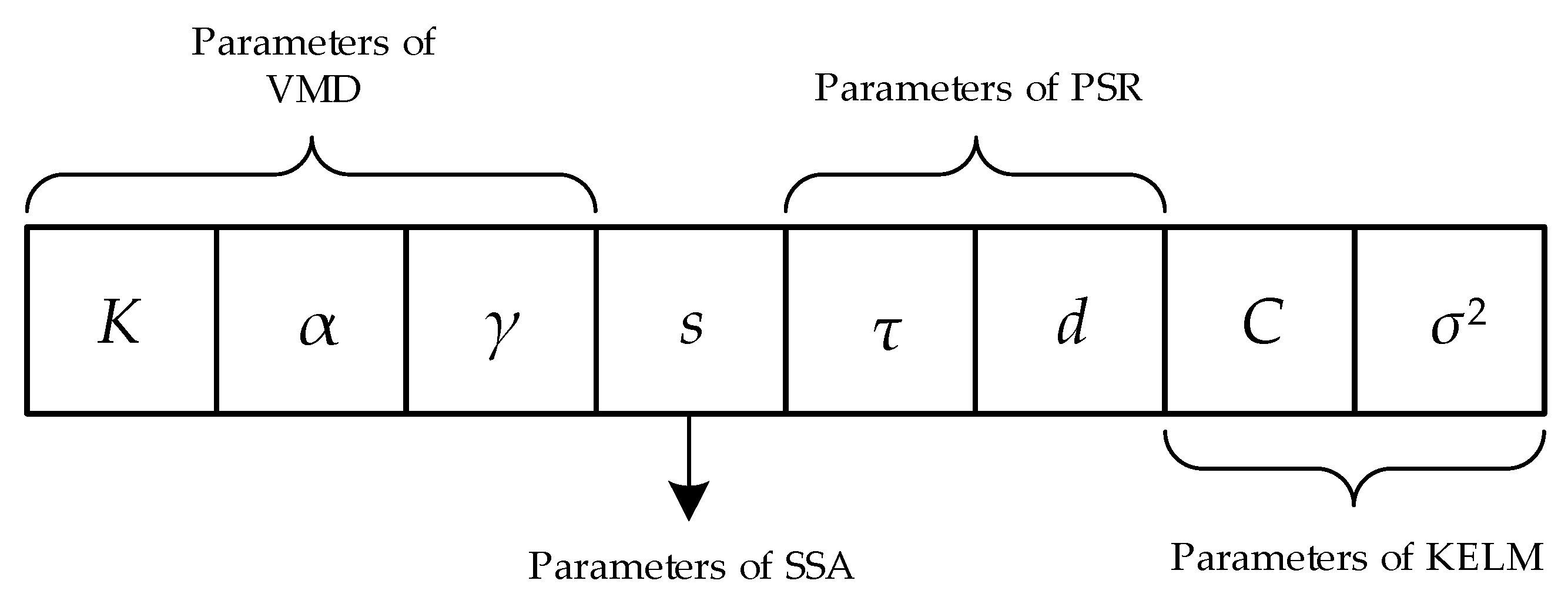
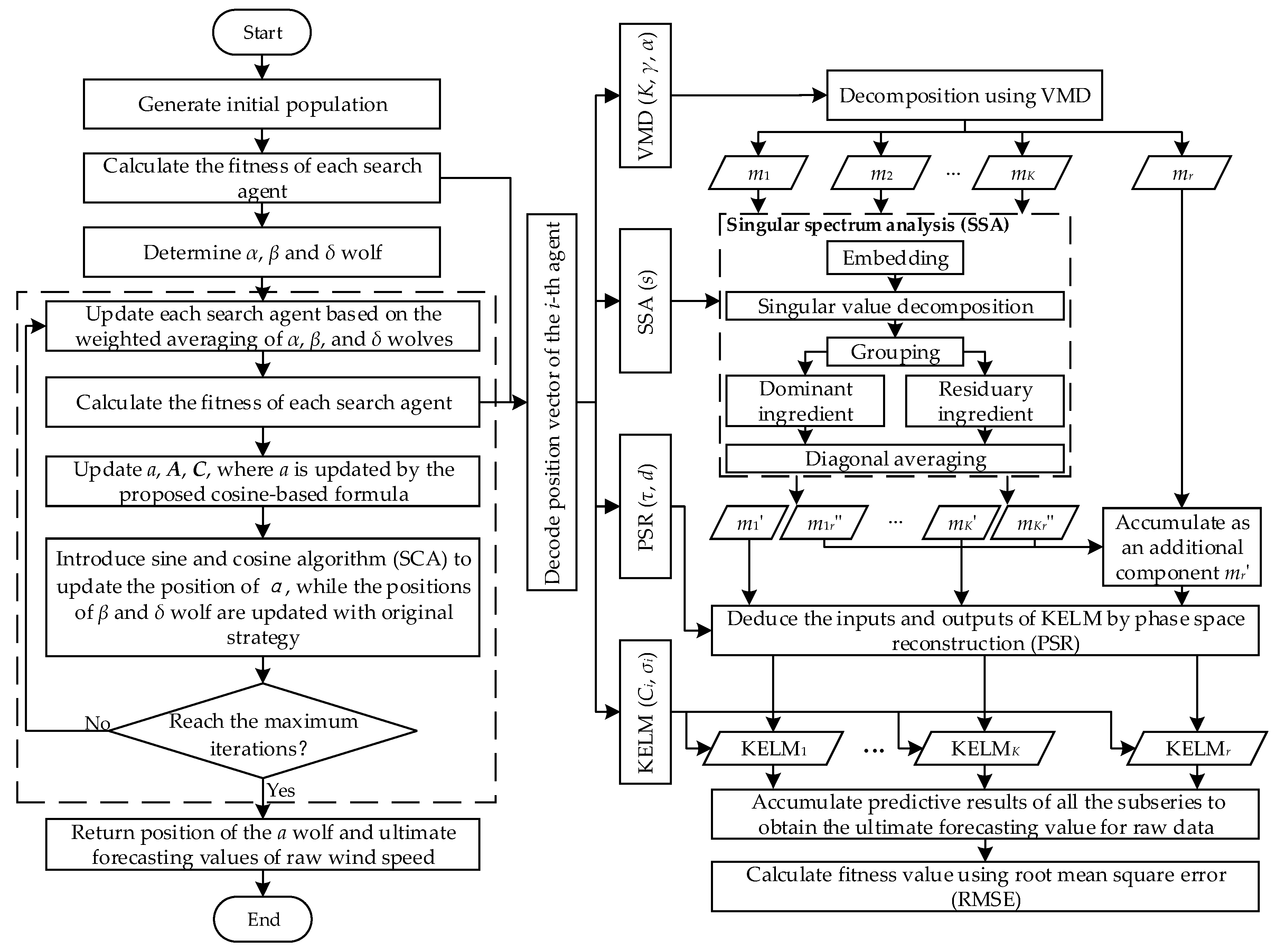
3. The Proposed Approach

3.1. Multi-Scale Dominant Ingredient Chaotic Analysis

Due to the non-linearity, non-stationarity, and random fluctuation characteristics within the wind speed time series, the forecasting performance would be severely restricted. Therefore, VMD is employed to preliminarily decompose the collected wind speed data into several sub-series with various frequency scales, of which the decomposition efficiency of VMD and the prediction accuracy are greatly affected by the parameters K, α and γ [21,22]. In order to further reduce the non-stationarity of the decomposed sub-series, SSA is implemented to extract the dominant ingredients and residuary ingredients from the sub-series, thus achieving multi-scale dominant ingredient analysis effectively. In this study, the set of indices Z = {1, 2, …, l} in the grouping phase of SSA is divided into two discrete subsets, that is, Z₁ = {1, 2, …, s} and Z₂ = {s + 1, s + 2, …, l}, with which the matrix H_Z could be represented as H_Z = H_Z1 + H_Z2. It is worth noting that the parameter s that determines the dominant ingredients could affect the prediction accuracy to some extent [36]. Additionally, the residual of VMD, i.e., $m_r=f-{{\displaystyle \sum }}_{k=1}^K{m}_k$ is integrated with all the residuary ingredients of all the sub-series for the ulterior improvement of the forecasting model’s capabilities. Subsequently, PSR, which has been widely utilized for chaotic time series analysis [9,37], is implemented to construct the inputs and outputs of the forecasting models, corresponding to each predictive component. Nevertheless, the time delay τ and the embedded dimension d could affect the recovery of the PSR dynamic system, with which the prediction performance would be significant restricted. It can be seen that the key to constructing the proposed hybrid forecasting model is to assign appropriate parameters to each module. To this end, an improved hybrid grey wolf optimizer-sine cosine algorithm (IHGWOSCA)-based synchronous optimization strategy is proposed, to achieve better parameter optimization and forecasting performance, which will be detailed later.

3.2. An Improved Hybrid Grey Wolf Optimizer-Sine Cosine Algorithm

The hybrid grey wolf optimizer-sine cosine algorithm (HGWO-SCA) is proposed by Singh et al. [38], of which both the grey wolf optimizer (GWO) and the sine cosine algorithm (SCA) are developed by Mirjalili et al. [39,40]. Four categories of grey wolves, α, β, δ, and ω are defined for simulating the leadership hierarchy in normal GWO, which are determined by the top three best positions (fitness value). Then, the equations that could be utilized for mathematically model encircling behavior are defined as below:

$$\stackrel{\rightharpoonup }{D}=\left|\stackrel{\rightharpoonup }{C}·\stackrel{\rightharpoonup }{X}p(t)-\stackrel{\rightharpoonup }{X}(t)\right|$$

(17)

$$\stackrel{\rightharpoonup }{X}(t+1)=\stackrel{\rightharpoonup }{X}p(t)-\stackrel{\rightharpoonup }{A}·\stackrel{\rightharpoonup }{D}$$

(18)

where t denotes the t-th iteration, ${\stackrel{\rightharpoonup }{X}}_p$ represents the position of the prey, $\stackrel{\rightharpoonup }{X}$ indicates the position vector of the grey wolf, and $\stackrel{\rightharpoonup }{A}$ and $\stackrel{\rightharpoonup }{C}$ are coefficient vectors calculated as follows:

$$\stackrel{\rightharpoonup }{A}=2\stackrel{\rightharpoonup }{a}·{\stackrel{\rightharpoonup }{r}}_1-\stackrel{\rightharpoonup }{a}$$

(19)

$$\stackrel{\rightharpoonup }{C}=2{\stackrel{\rightharpoonup }{r}}_2$$

(20)

where r₁ and r₂ are random vectors in the scopes of [0, 1]; the components of $\stackrel{\rightharpoonup }{a}$ linearly decrease from 2 to 0 over the course of the iteration in the normal GWO and HGWO-SCA. Besides, the transition between the exploration and exploitation stage depends on the components of $\stackrel{\rightharpoonup }{a}$ and $\stackrel{\rightharpoonup }{A}$, of which half of the iterations are divided toward exploration, when $\stackrel{\rightharpoonup }{\left|\mathrm{A}\right|}>1$ and the remaining iterations are assigned for exploitation when $\stackrel{\rightharpoonup }{\left|\mathrm{A}\right|}<1$ [39]. Hence, to better improve the corresponding abilities of these two phases, a cosine function-based decreasing formula for updating the components of $\stackrel{\rightharpoonup }{a}$ is proposed in this study:

$$a=1+\cos (\pi ·\frac{t}{T})$$

(21)

where t and T represent the current iteration and the maximum number of iterations, respectively. In addition, the comparison of the proposed function and the original one for updating the components of $\stackrel{\rightharpoonup }{a}$ over the course of the iterations is intuitively exhibited in Figure 1. As can be seen from Figure 1, the values of $\stackrel{\rightharpoonup }{a}$ are generally larger in the proposed function during the first half of the iterations, which could contribute to improving the exploration ability of the algorithm at this stage. The corresponding effects in the exploitation phase would be obtained with smaller values of $\stackrel{\rightharpoonup }{a}$, compared to the original ones.

The other stage of the whole algorithm, namely hunting, is usually guided by the α wolf, while the β and δ wolves participate in hunting occasionally [39]. To effectively mathematically simulate the hunting behavior, the α, β, and δ wolves are assumed to possess more knowledge about the potential location of prey. In addition, the position updating functions of the α wolf in HGWO-SCA are modified by applying the position updating equations of SCA, thus enhancing the convergence capabilities of GWO [38]. The corresponding updating equations of the α, β, and δ wolves are defined as follows:

$${\stackrel{\rightharpoonup }{D}}_{\alpha }=\{\begin{array}{ll}rand()\times \sin (0.5\times \pi \times rand())\times \left|{\stackrel{\rightharpoonup }{C}}_1\times {\stackrel{\rightharpoonup }{X}}_{\alpha }-\stackrel{\rightharpoonup }{X}\right|,& rand()<0.5\\ rand()\times \cos (0.5\times \pi \times rand())\times \left|{\stackrel{\rightharpoonup }{C}}_1\times {\stackrel{\rightharpoonup }{X}}_{\alpha }-\stackrel{\rightharpoonup }{X}\right|,& rand()\ge 0.5\end{array}$$

(22)

$${\stackrel{\rightharpoonup }{D}}_{\beta }=\left|{\stackrel{\rightharpoonup }{C}}_2\times {\stackrel{\rightharpoonup }{X}}_{\beta }-\stackrel{\rightharpoonup }{X}\right|;{\stackrel{\rightharpoonup }{D}}_{\delta }=\left|{\stackrel{\rightharpoonup }{C}}_3\times {\stackrel{\rightharpoonup }{X}}_{\delta }-\stackrel{\rightharpoonup }{X}\right|$$

(23)

$${\stackrel{\rightharpoonup }{X}}_1={\stackrel{\rightharpoonup }{X}}_{\alpha }-{\stackrel{\rightharpoonup }{A}}_1·{\stackrel{\rightharpoonup }{D}}_{\alpha };{\stackrel{\rightharpoonup }{X}}_2={\stackrel{\rightharpoonup }{X}}_{\beta }-{\stackrel{\rightharpoonup }{A}}_2·{\stackrel{\rightharpoonup }{D}}_{\alpha };{\stackrel{\rightharpoonup }{X}}_3={\stackrel{\rightharpoonup }{X}}_{\delta }-{\stackrel{\rightharpoonup }{A}}_3·{\stackrel{\rightharpoonup }{D}}_{\delta }$$

(24)

where ${\stackrel{\rightharpoonup }{X}}_1$, ${\stackrel{\rightharpoonup }{X}}_2$ and ${\stackrel{\rightharpoonup }{X}}_3$ indicate the positional information owned by the α, β, and δ wolves so far. Due to the fact that individuals in HGWO-SCA are merely updated by simple averaging ${\stackrel{\rightharpoonup }{X}}_1$, ${\stackrel{\rightharpoonup }{X}}_2$ and ${\stackrel{\rightharpoonup }{X}}_3$, some scholars have focused on the updating approaches for the individuals [41]. In this study, a weighted averaging strategy is proposed to iterate the individuals, in which α, β, and δ wolves are separately assigned a weight value that is deduced by inversing the corresponding fitness values of the wolves. The detailed calculations are as follows:

$$w_{\alpha }=\frac{1}{fi{t}_{\alpha }},w_{\beta }=\frac{1}{fi{t}_{\beta }},w_{\delta }=\frac{1}{fi{t}_{\delta }}$$

(25)

$$\overrightarrow{X}(t+1)=\frac{w_{\alpha }·{\overrightarrow{X}}_1(t)+w_{\beta }·{\overrightarrow{X}}_2(t)+w_{\delta }·{\overrightarrow{X}}_3(t)}{w_{\alpha }+w_{\beta }+w_{\delta }}$$

(26)

where fit denotes the fitness of the corresponding individual. Furthermore, the pseudo code of the proposed IHGWOSCA algorithm is exhibited in Algorithm 1.

Algorithm 1. The pseudo code of the proposed IHGWOSCA algorithm
1:	Initialization the population ${\stackrel{\rightharpoonup }{X}}_i$ (i = 1, 2, …, N)
2:	Initialize a, $\stackrel{\rightharpoonup }{A}$ and $\stackrel{\rightharpoonup }{C}$
3:	Calculate the fitness of each search member
4:	${\stackrel{\rightharpoonup }{X}}_{\alpha }$: the best search agents, ${\stackrel{\rightharpoonup }{X}}_{\beta }$: the second-best search agent, ${\stackrel{\rightharpoonup }{X}}_{\delta }$: the third-best search agent
5:	While (t < maximum number of iterations)
6:	For each search agent:
7:	Update the position of the current search agent on the basis of Equations (25) and (26)
8:	End for:
9:	Update a, $\stackrel{\rightharpoonup }{A}$, and $\stackrel{\rightharpoonup }{C}$ by Equations (21), (19) and (20), respectively.
10:	Calculate the fitness of all grey wolves
11:	Save the position information owned by the β and δ wolves with Equations (23) and (24), while the position information for α wolf are updated as below:
12:	If rand () < 0.5
13:	Then:
14	${\stackrel{\rightharpoonup }{D}}_{\alpha }$ = rand () × sin (0.5⋅π⋅rand ()) × |${\stackrel{\rightharpoonup }{C}}_1$ × ${\stackrel{\rightharpoonup }{X}}_{\alpha }$ − $\stackrel{\rightharpoonup }{D}$|
15:	Else:
16:	${\stackrel{\rightharpoonup }{D}}_{\alpha }$ = rand () × cos (0.5⋅π⋅rand ()) × |${\stackrel{\rightharpoonup }{C}}_1$ × ${\stackrel{\rightharpoonup }{X}}_{\alpha }$ − $\stackrel{\rightharpoonup }{D}$|
17:	${\stackrel{\rightharpoonup }{X}}_1$ = ${\stackrel{\rightharpoonup }{X}}_{\alpha }$ − ${\stackrel{\rightharpoonup }{A}}_1$ · ${\stackrel{\rightharpoonup }{D}}_{\alpha }$
18:	End if
19:	End else
20:	t = t+1
21:	End while
22:	Return ${\stackrel{\rightharpoonup }{X}}_{\alpha }$

3.3. Optimization Strategy

In order to effectively optimize the parameters in various modules, as well as construct the hybrid forecasting model, the proposed IHGWOSCA algorithm is adopted to handle this problem. To begin with, the parameters of SSA, PSR, and KELM for all the sub-series are considered to be the same in this study, which could facilitate fast convergence as well as reduce computation. Hence, the total number of the variables is eight, while the corresponding coding strategy of the agents in the proposed IHGWOSCA is described in Figure 2. Additionally, the metric root-mean-square error (RMSE) represented in Equation (27) is adopted as the objective function for parameter optimization.

3.4. Specific Procedures

The main procedures of the proposed novel hybrid wind speed forecasting model, combined with VMD, SSA, PSR, KELM, and IHGWOSCA-based synchronous optimization strategies are described as follows:

Step 1: Collect the original wind speed data and initialize the population of IHGWOSCA;

Step 2: Calculate the fitness value for each agent;

Step 2.1: Decode the population and assign the corresponding parameters for each module, i.e., the parameters K, α, γ for VMD, s for SSA, τ, d for PSR as well as C, and σ² for KELM;

Step 2.2: Decompose the collected wind speed data into K modes by utilizing VMD, then calculate the residual m_r of VMD;

Step 2.3: Implement SSA for all the sub-series, then extract the dominant ingredients as well as accumulate all of the residuary ingredients with m_r.

Step 2.4: For the k-th (k = 1, …, K, K + 1) component, construct the input and output matrixes for the k-th (k = 1, …, K, K + 1) KELM, applying PSR;

Step 2.5: Model the k-th (k = 1, …, K, K + 1) KELM with parameters C and σ². Repeat Steps 2.4 to 2.5 until k = K + 1, then accumulate the predicted results of all the components to obtain the ultimate forecasting value, and then calculate the fitness value by Equation (27).

Step 2.6: Repeat Steps 2.1 to 2.5 until the fitness values for all the agents are generated;

Step 3: Execute the operators of IHGWOSCA.

Step 4: Repeat Step 2 to 3 until the maximum number of iterations is reached;

Step 5: Obtain the optimal parameters for all of the modules by decoding the best individual, as well as calculate the final forecasting values of the collected wind speed data by repeating Steps 2.1 to 2.5.

The overall process of the proposed wind speed forecasting model is depicted in Figure 3.

4. Experimental Design

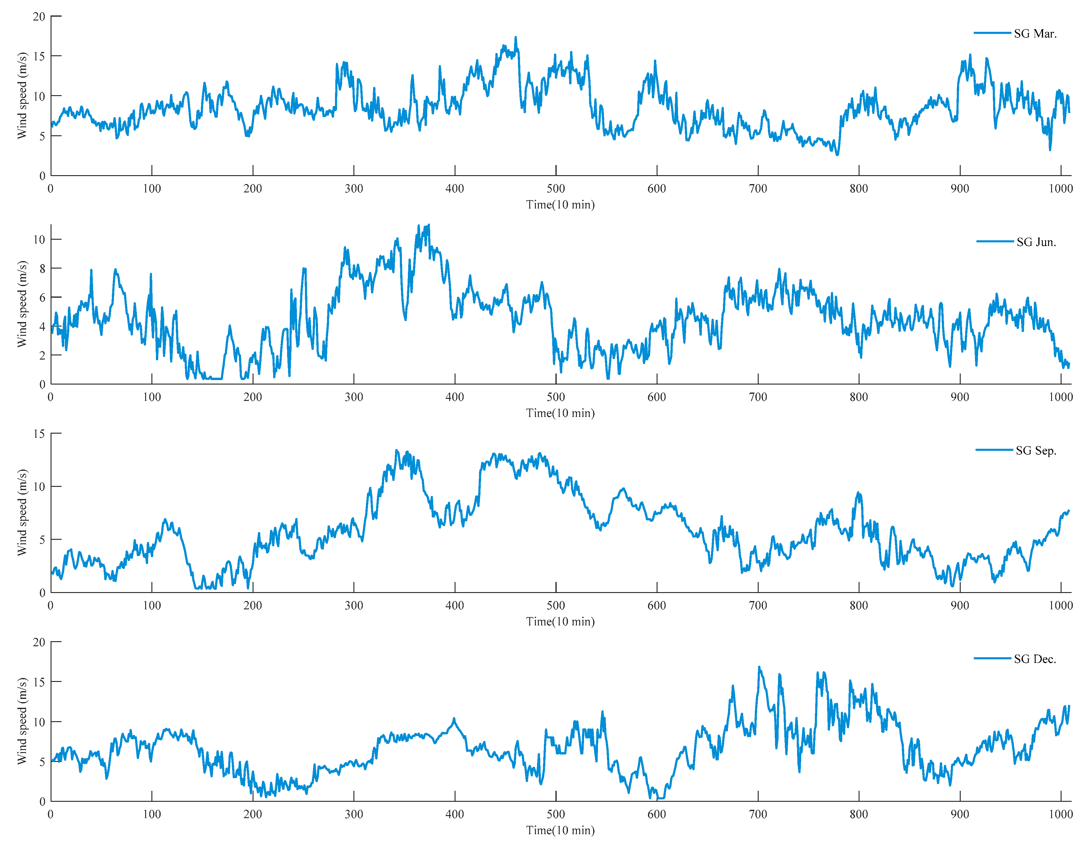
4.1. Data Collection

In this study, four cases of short-term wind speed data are collected from Sotavento Galicia (SG) wind farm, of which the data are recorded with a mean time interval of 10 minutes. Furthermore, these four cases are selected from SG for the time periods of 8–14 March, 7–13 June, 22–28 September, 8–14 December in 2018, which are named as SG Mar., SG Jun., SG Sep. and SG Dec. in the later experiments, respectively. The visualizations of all of the collected wind speed time series are shown in Figure 4, and the corresponding statistical information including the maximum (Max.) value, minimum (Min.) value, mean value, skewness (Skew.), kurtosis (Kurt.), and standard deviation (Std.) are exhibited in

Table 1. Statistical information for the four datasets from SG.

Cases	Statistic Indices
	Max. (m/s)	Min. (m/s)	Mean (m/s)	Stew.	Kurt.	Std.
SG March	17.38	2.56	8.53	0.56	2.96	2.68
SG June	11.00	0.35	4.5	0.27	2.94	2.13
SG September	13.39	0.35	5.77	0.6	2.6	3.19
SG December	16.84	0.35	6.7	0.44	3.21	3.12

. It can be intuitively observed that the raw wind speed time series possesses strong non-linearity and non-stationarity, with which the precise forecasting model would be difficult to construct. Additionally, the phase space matrices corresponding to the forecasting components are deduced by PSR with various parameters, among which the last 288 samples are assigned to be the testing sets in all of the experimental cases.

4.2. Experimental Description

In order to testify the availability of the proposed hybrid prediction model based on the VMD, SSA, PSR, KELM, and IHGWOSCA-based synchronous optimization strategies, a set of single models and combined models are carried out for comparative experiments in one-step, three-step, and five-step predictions. The single models, namely SVR and KELM are directly adopted for prediction, of which the parameters in both of these two models are searched by grid search (GS). The remaining four combine comparative models integrating with various assistive technologies, including EMD-KELM, VMD-KELM, EMD-SSA-PSR-KELM, and VMD-SSA-PSR-KELM are utilized to demonstrate the availability of the proposed modified modules. Among these combined models, both EMD-KELM and EMD-SSA-PSR-KELM achieved wind speed forecasting with the EMD-based decomposition method, while the former one used KELM for prediction modeling without SSA, whereas KELM and the proposed dominant ingredient chaotic analysis were adopted in the latter one. Both VMD-KELM and VMD-SSA-PSR-KELM are based on the VMD decomposition technique, while the only difference between the two is that the proposed dominant ingredient chaotic analysis combining SSA and PSR is employed in latter one, while the former one is not implemented.

In order to assess the performance of all the forecasting models quantitatively, three common indexes, including RMSE, mean absolute error (MAE), and mean absolute percentage error (MAPE) are employed, which could measure the deviation between the predicted and collected values [42]. The detailed equations of these three metrics are described as follows:

$$RMSE=\sqrt{\frac{1}{N}{\displaystyle {\sum }_{i=1}^N{(Y_i-{\widehat{Y}}_i)}^2}}$$

(27)

$$MAE=\frac{1}{N}{\displaystyle {\sum }_{i=1}^N\left|Y_i-{\widehat{Y}}_i\right|}$$

(28)

$$MAPE=\frac{1}{N}{\displaystyle {\sum }_{i=1}^N\left|\frac{100\times (Y_i-{\widehat{Y}}_i)}{Y_i}\right|}$$

(29)

where N denotes the total number of testing samples, and Y and $\widehat{Y}$ represent the collected and predicted values, respectively. Additionally, the reducing ratios of the indexes RMSE, MAE, and MAPE are employed to evaluate the performance between two different models [1,43,44], with which the improvement degree of the proposed model could be quantitatively expressed. The detailed definitions of these percentage-based indexes, including P_RMSE, P_MAE, and P_MAPE are as follows:

$$P_{RMSE}=\left(\frac{RMS{E}_a-RMS{E}_b}{RMS{E}_a}\right)\times 100$$

(30)

$$P_{MAE}=\left(\frac{MA{E}_a-MA{E}_b}{MA{E}_a}\right)\times 100$$

(31)

$$P_{MAPE}=\left(\frac{MAP{E}_a-MAP{E}_b}{MAP{E}_a}\right)\times 100$$

(32)

where the subscript a denotes the comparative model, and subscript b represents the proposed model in this study.

For the proposed model, the search agents and the maximum iterations of IHGWOSCA are given as 10 and 20, respectively. The predetermined parameters of the window length l for Hankel matrix in SSA is set as 500. The parameters (K, α, γ) in VMD, (s) in SSA, (τ, d) in PSR, and (C, σ²) in KELM are searched for the scopes of [2, 10], [0, 1], [1, 2000], [1, 167], [1, 15], [1, 40], [1, 1000], and [1, 1000], orderly. For the relevant comparative models, the regularization coefficient C and the kernel parameter σ² of all the SVR- and KELM-based models are optimized by GS, where the searching scopes are in intervals [2⁻⁸, 2⁸] and [2⁻⁵, 2⁵], respectively. For the VMD-based comparative models, the parameter α is set as the default value of 2000, and the parameters K and γ are optimized by GS [13], of which K is searched in [2, 10] with increasing step 1, and γ is searched in [0, 1] with increasing step 0.1. Meanwhile, for the SSA- and PSR-based models, including EMD-SSA-PSR-KELM and VMD-SSA-PSR-KELM, the window length l of the Hankel matrix is given as 500, and the corresponding parameter s is set as 105, as suggested in [36]. Besides, the parameters τ and d of PSR are set as 1 and 10, respectively. Furthermore, the optimal parameters within the proposed models are obtained by the proposed IHGWOSCA algorithm in different horizons for all experimental cases, as illustrated in

Table 2. Optimal parameters of the proposed models in different prediction horizons for all of the experimental cases.

Cases	Horizons	Parameters
		K	α	γ	s	τ	d	C	σ2
SG March	One-step	10	877	0.98	167	1	13	358.13	118.06
	Three-step	10	770	0.19	118	1	26	514.82	242.26
	Five-step	10	968	0.29	117	1	15	419.53	129.29
SG June	One-step	10	645	0.43	167	1	15	1000	129.48
	Three-step	10	1213	0.91	93	1	6	1000	52.61
	Five-step	10	62	0.48	64	1	31	829.72	166.47
SG September	One-step	10	213	0.79	154	1	12	1000	43.67
	Three-step	10	127	0.4	86	1	18	988.64	330.17
	Five-step	10	122	0.09	84	1	14	875.89	129.23
SG December	One-step	10	728	0.99	167	1	9	1000	201.19
	Three-step	10	223	0.94	83	1	10	686.65	116.63
	Five-step	10	531	0.61	53	1	13	688.51	263.35

.

4.3. Contrasting Analyses

In this section, the results of the one-step, three-step, and five-step forecasting on all of the experimental cases are discussed in detail. The metrics RMSE, MAE, and MAPE, obtained by all of the comparative models and the proposed model with various prediction horizons are illustrated in

Table 3. Results of multi-step forecasting on the test data in all cases.

Cases	Models	One-Step			Three-Step			Five-Step
		RMSE	MAE	MAPE	RMSE	MAE	MAPE	RMSE	MAE	MAPE
		(m/s)	(m/s)	(%)	(m/s)	(m/s)	(%)	(m/s)	(m/s)	(%)
SG March	SVR	1.06	0.81	11.37	1.53	1.18	17.33	1.83	1.42	21.29
	KELM	1.05	0.80	10.35	1.50	1.16	15.20	1.76	1.36	17.67
	EMD-LSSVM	0.68	0.50	6.54	0.83	0.64	8.43	1.05	0.80	10.39
	VMD-KELM	0.12	0.09	1.21	0.19	0.15	1.98	0.33	0.26	3.44
	EMD-SSA-PSR-KELM	0.52	0.38	4.71	0.80	0.60	7.69	0.93	0.70	9.12
	VMD-SSA-PSR-KELM	0.08	0.06	0.84	0.17	0.14	1.87	0.30	0.24	3.11
	Proposed	0.06	0.05	0.65	0.16	0.13	1.71	0.27	0.20	2.61
SG June	SVR	0.64	0.52	13.69	0.93	0.74	19.79	0.97	0.77	22.05
	KELM	0.63	0.51	12.76	0.88	0.71	17.41	0.96	0.76	18.37
	EMD-LSSVM	0.36	0.28	7.27	0.48	0.39	10.07	0.54	0.44	11.34
	VMD-KELM	0.05	0.04	1.00	0.11	0.09	2.29	0.20	0.16	4.24
	EMD-SSA-PSR-KELM	0.22	0.17	4.40	0.43	0.33	8.96	0.49	0.39	10.22
	VMD-SSA-PSR-KELM	0.04	0.03	0.75	0.10	0.08	2.08	0.17	0.13	3.60
	Proposed	0.03	0.02	0.61	0.09	0.07	1.82	0.11	0.09	2.33
SG September	SVR	0.63	0.45	13.44	0.97	0.71	23.04	1.27	0.97	29.97
	KELM	0.61	0.44	11.96	0.96	0.71	18.91	1.19	0.91	23.27
	EMD-LSSVM	0.42	0.29	9.29	0.58	0.41	12.20	0.71	0.53	14.98
	VMD-KELM	0.08	0.06	1.70	0.12	0.09	2.76	0.20	0.16	4.69
	EMD-SSA-PSR-KELM	0.33	0.22	7.21	0.49	0.34	10.58	0.65	0.47	13.67
	VMD-SSA-PSR-KELM	0.07	0.05	1.40	0.10	0.08	2.25	0.18	0.14	4.37
	Proposed	0.03	0.03	0.70	0.08	0.06	1.93	0.12	0.09	2.76
SG December	SVR	1.23	0.89	12.29	1.89	1.38	18.95	2.22	1.63	21.96
	KELM	1.22	0.89	12.01	1.89	1.37	18.28	2.15	1.57	20.53
	EMD-LSSVM	0.63	0.50	6.76	0.90	0.68	9.30	1.12	0.85	11.87
	VMD-KELM	0.16	0.12	1.71	0.32	0.24	3.24	0.50	0.37	5.14
	EMD-SSA-PSR-KELM	0.41	0.31	4.24	0.74	0.55	7.35	0.99	0.73	10.18
	VMD-SSA-PSR-KELM	0.14	0.10	1.33	0.29	0.21	2.81	0.47	0.35	4.75
	Proposed	0.09	0.07	0.87	0.22	0.16	2.28	0.36	0.28	3.72

, respectively, of which the proposed models are highlighted in bold. Meanwhile, in order to assess the improvements that are achieved by the proposed model compared with the comparative models, the performance improvements are depicted in

Table 4. Percentage of the promotion between the comparative models and the proposed model in all experimental cases for multi-step prediction.

Cases	Extant Models vs Proposed	One-Step			Three-Step			Five-Step
		PRMSE (%)	PMAE (%)	PMAPE (%)	PRMSE (%)	PMAE (%)	PMAPE (%)	PRMSE (%)	PMAE (%)	PMAPE (%)
SG March	SVR	94.03	94.11	94.31	89.38	89.23	90.14	84.97	85.56	87.74
	KELM	93.97	94.00	93.75	89.19	88.97	88.76	84.42	84.98	85.23
	EMD-KELM	90.70	90.50	90.11	80.46	80.2	79.74	73.95	74.61	74.86
	VMD-KELM	47.03	47.76	46.56	15.78	15.39	13.89	17.91	21.75	24.18
	EMD-SSA-PSR-KELM	87.78	87.32	86.26	79.71	78.72	77.78	70.60	70.97	71.37
	VMD-SSA-PSR-KELM	22.14	24.49	23.05	5.97	8.07	8.71	9.28	14.41	15.94
SG June	SVR	95.45	95.58	95.57	90.58	90.84	90.81	88.59	88.81	89.41
	KELM	95.40	95.55	95.25	90.05	90.49	89.56	88.44	88.73	87.29
	EMD-KELM	91.98	91.87	91.66	81.96	82.87	81.94	79.48	80.30	79.41
	VMD-KELM	41.97	42.32	39.64	20.05	23.03	20.50	44.31	46.62	44.89
	EMD-SSA-PSR-KELM	86.89	86.49	86.22	79.55	79.83	79.72	77.25	78.07	77.16
	VMD-SSA-PSR-KELM	21.68	22.90	19.68	12.17	16.25	12.80	33.13	35.72	35.12
SG September	SVR	94.51	94.29	94.81	91.63	90.92	91.62	90.60	90.52	90.79
	KELM	94.32	94.16	94.17	91.55	90.88	89.79	89.95	89.82	88.14
	EMD-KELM	91.85	91.24	92.50	85.97	84.28	84.17	83.14	82.53	81.57
	VMD-KELM	56.66	56.78	58.96	34.81	30.39	30.04	40.35	41.00	41.18
	EMD-SSA-PSR-KELM	89.39	88.60	90.33	83.41	81.26	81.75	81.52	80.39	79.81
	VMD-SSA-PSR-KELM	48.58	49.90	50.28	19.70	17.39	14.26	35.44	35.70	36.76
SG December	SVR	92.97	92.63	92.90	88.56	88.14	87.96	83.73	82.99	83.08
	KELM	92.90	92.6	92.73	88.51	88.05	87.52	83.23	82.39	81.91
	EMD-KELM	86.26	86.91	87.09	75.87	76.03	75.46	67.82	67.33	68.70
	VMD-KELM	45.80	45.89	48.98	32.69	30.69	29.62	27.79	25.07	27.76
	EMD-SSA-PSR-KELM	79.08	78.98	79.41	70.56	70.06	68.95	63.47	62.22	63.50
	VMD-SSA-PSR-KELM	39.04	34.46	34.56	25.47	22.39	18.69	24.07	19.98	21.72

integrally. As can be observed from Table 3 and Table 4, several consequences could be drawn as below:

(1)

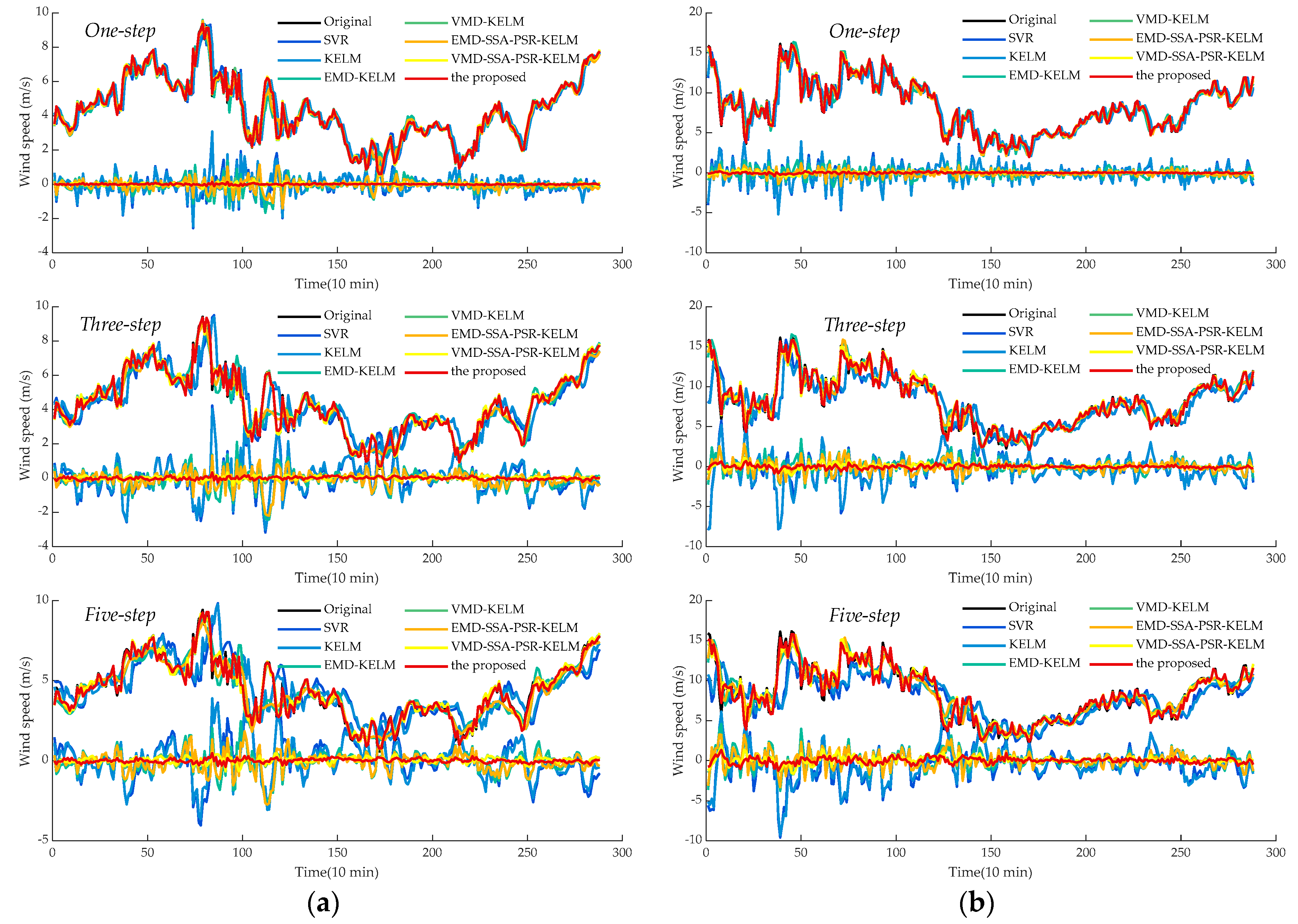
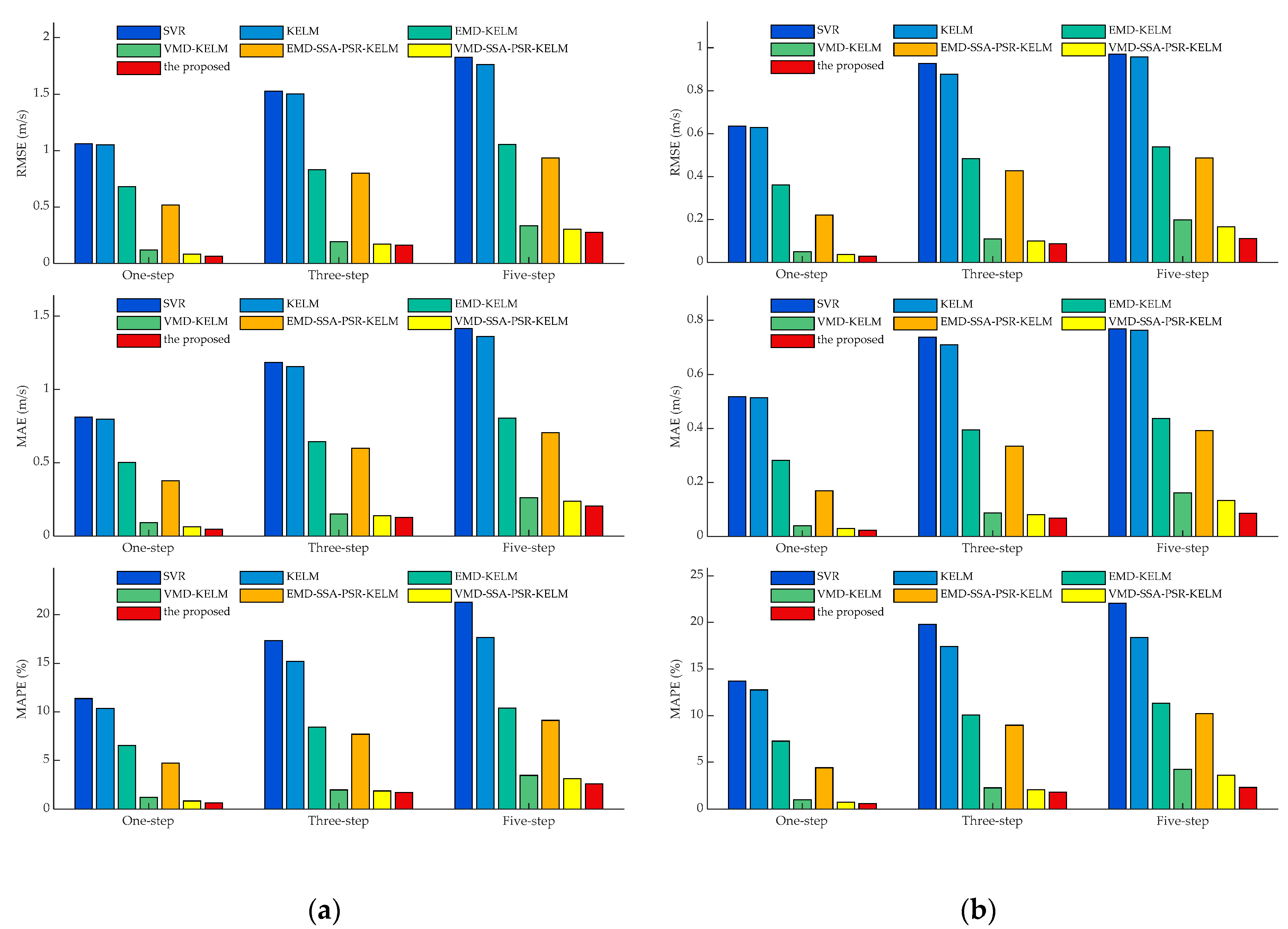
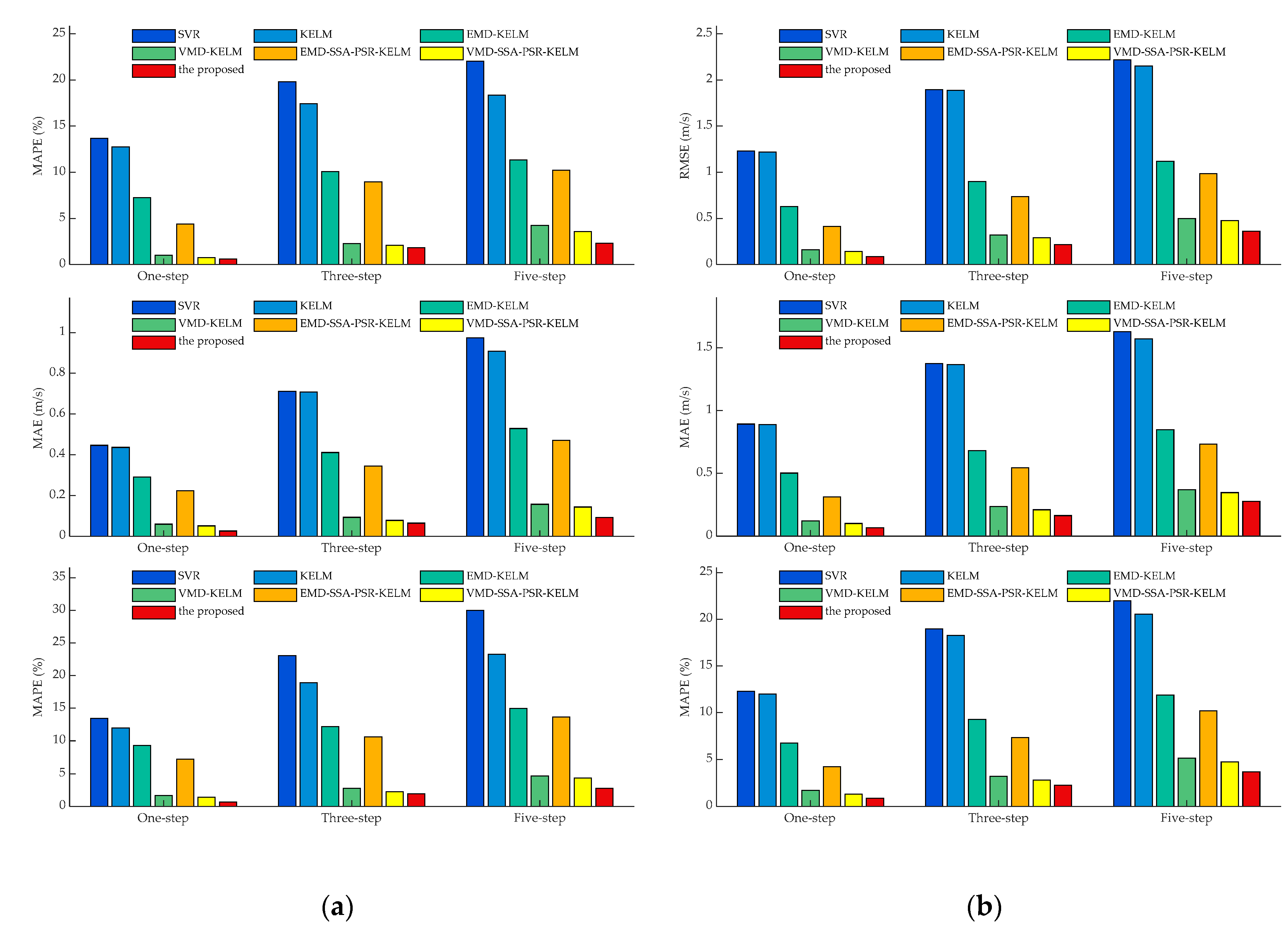
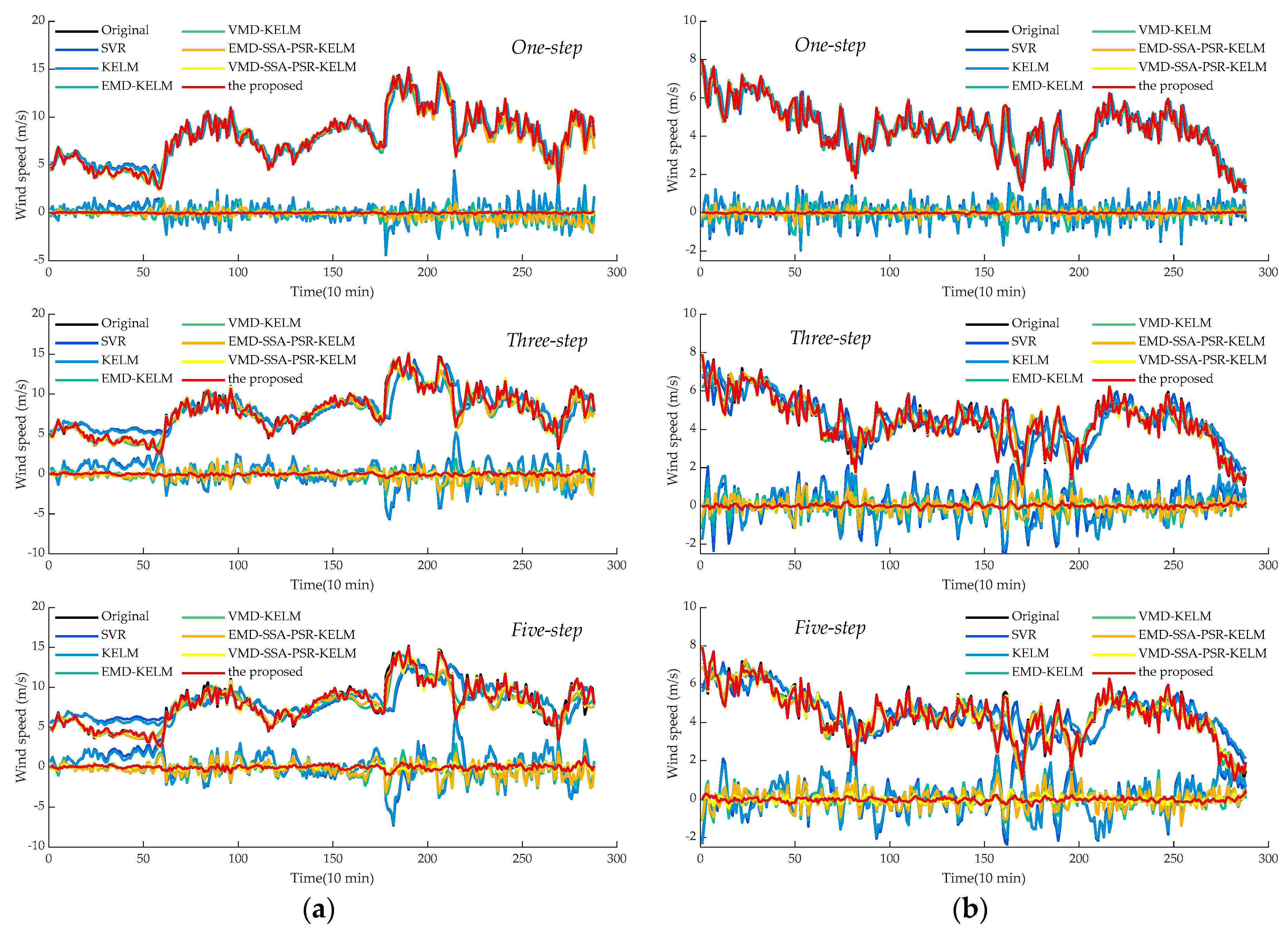
Comparing the metrics RMSE, MAE, and MAPE, obtained by SVR and KELM in all experimental cases, it can be observed that KELM generally possesses lower metrics than SVR, which means that a better forecasting performance could be obtained by KELM. For instance, in the cases of SG Mar. and SG Jun., the one-step prediction results in terms of MAPE for these two models are 11.37%, 10.35%, and 13.69% 12.76%, of which the reducing ratios of MAPE for KELM are 8.92% and 6.75%, respectively. Furthermore, this trend would be pronounced in the multi-step predictions. In the three-step and five-step predictions in the case of SG Sep., the three employed indicators obtained by SVR and KELM are 0.97 m/s, 0.71 m/s, 23.04% (SVR, three-step), 0.96 m/s, 0.71 m/s, 18.91% (KELM, three-step) and 1.27 m/s, 0.97 m/s, 29.97 (SVR, five-step), 1.19 m/s, 0.91 m/s, 23.27% (KELM, five-step) orderly. It can be seen that the decreasing percentages of the index MAPE for KELM in three-step and five-step forecasting are 17.91% and 22.37%, respectively, with which the superiority of KELM could be demonstrated effectively. It is worth noting that satisfactory results could not be directly achieved by the single models such as SVR and KELM, which could be attributed to the strong non-stationarity and non-linearity of the original wind speed time series. To this end, signal preprocessing technologies are necessary to enhance prediction performance.

(2)

Following the comparison of KLEM, EMD-KELM and VMD-KELM, it can be indicated that time-frequency signal processing approaches could greatly improve the prediction accuracy for wind speed. In the case of SG Dec., the evaluation metrics obtained by EMD-KELM in one-step predictions are 0.63 m/s, 0.50 m/s, 6.76%, which are deceased by 48.37%, 43.45%, and 43.74%, compared to the single-model KELM. Meanwhile, the metrics reducing ratio in the three-step and five-step predictions obtained by comparing KELM and EMD-KELM are 52.37%, 50.16%, 49.15% and 47.87%, 46.07%, and 42.20%, respectively. From further comparison of the results of EMD-KELM and VMD-KELM, it can be indicated that the three evaluation indicators obtained by VMD-KELM are decreased by averaging 75.05%, 64.90%, and 56.17% in three experimental prediction horizons, respectively. Hence, it can be concluded that VMD could improve the forecasting accuracy better than EMD. Similar conclusions could be drawn by the same analysis for the remaining experimental cases.

(3)

The proposed dominant ingredient chaotic analysis combining SSA and PSR could improve the prediction model performance in an ulterior manner. In the case of SG Mar., compared with EMD-KELM, the metrics obtained by EMD-SSA-PSR-KELM are 0.52 m/s, 0.38 m/s, 4.71%, 0.80 m/s, 0.60 m/s, 7.69%, 0.93 m/s, 0.70 m/s, 9.12% in three variously predicted horizons, of which the corresponding decreasing percentages are averaged by 25.67%, 6.50% and 12.04%. Meanwhile, compared with VMD-KELM, the metrics of VMD-SSA-PSR-KELM have been averaged, decreasing by 31.11%, 8.02% and 9.30% in different predicted horizons, respectively. The comparisons of EMD-KELM, EMD-SSA-PSR-KELM and VMD-KELM, and VMD-SSA-PSR-KELM indicate that the proposed dominant ingredient chaotic analysis could further enhance the forecasting performance on the basis of the signal decomposition approaches implemented. Nevertheless, the performance of the proposed dominant ingredient chaotic analysis would be restricted by the parameters that are settled in SSA and PSR, which makes parameter optimization necessary.

(4)

Comparing VMD-SSA-PSR-KELM and the proposed model, both of these two models possess the same frameworks, while the parameters in the proposed one are optimized by the proposed IHGWOSCA algorithm synchronously. In the case of SG Mar. as the example, the metrics decreasing the percentage between VMD-SSA-PSR-KELM and the proposed model in terms of MAPE are 23.05%, 8.71%, and 15.94% in three predicted horizons, respectively. It can be concluded that the forecasting performance obtained by the synchronous optimization strategy-based model is much better; in other words, the appropriate parameters in each module could be optimized by the proposed IHGWOSCA effectively. Additionally, for one-step prediction in all cases, the average decline ratios between these two models in terms of RMSE, MAE, and MAPE are 32.86%, 32.94%, 31.89%, respectively. Furthermore, compared with SVR models in all experimental cases, the maximum decreasing ratio of MAPE in the one-, three- and five-step predictions are 95.57% (in the case of SG Jun.), 91.62% (in the case of SG Sep.), and 90.79% (in the case of SG Sep.), respectively, with which it can be indicated that a large promotion in performance could be achieved by the proposed model.

Additionally, in order to achieve intuitive observation of the forecasting results, the curves of the predicted and collected values, as well as prediction errors of all experimental models were depicted in Figure 5 and Figure 6. As can be observed, the predicted curves of the proposed model in both single-step and multi-step forecasting could better approximate real curves, while the corresponding forecasting errors are evenly distributed around zero with small fluctuations. It can be indicated that the forecasting performance of the proposed model does not decrease significantly with the increase of the prediction step size, with which the superiority of the proposed model could be demonstrated convincingly.

Furthermore, the histograms of the metrics RMSE, MAE, and MAPE obtained by all of the experimental models with various prediction horizons, are shown in Figure 7 and Figure 8, with which the variation tendencies of the evaluation indicators over the course of increasing prediction horizons could be observed intuitively. It can be observed that the indexes values obtained by the proposed model achieved minimums in all of the experiments, while the same framework-based VMD-SSA-PSR-KELM models achieved suboptimal performance in all experiments. Besides, the time–frequency signal decomposition-based models generally possess lower index values in terms of RMSE, MAE, and MAPE, while the performance improvements brought by VMD are much more than EMD, in this study. In addition, the proposed dominant ingredient, chaotic analysis combining SSA and PSR, could act as an ulterior force to enhance the forecasting performance to some extent, while the promotion caused by the analysis approach would be significant if the parameters of SSA and PSR were appropriately set. Furthermore, such parameter-searching problems could be effectively solved by the proposed IHGWOSCA algorithm, based on the synchronous optimization strategy.

5. Discussion

Following the detailed comparative analyses that are depicted above, the superiority of the proposed hybrid approach combining the VMD, SSA, PSR, KELM, and IHGWOSCA-based synchronous optimization strategies could be demonstrated effectively. It is worth noting that there exist only one kind of forecasting model in the proposed approach; i.e., the AI model, while the strategy of mixing various categories of prediction models such as AI and physical models was not considered in this study. According to the past references [45,46,47], such mixed models have been widely investigated for enhancing the prediction accuracy. Among the models, the advantages corresponding to each model could be maximized, thus making full use of each model to deal with different situations. In addition, the proposed IHGWOSCA algorithm could be optimized with better strategies for further enhancing the convergence speed, as well as the global search capability. Furthermore, multi-objective optimization that has been widely utilized in the field of controlling [48] could be implemented in wind speed forecasting, which could contribute to enhancing the performance of the models [49]. Therefore, several perspectives for further investigation directions could be summarized as: (1) the combination of multiple forecasting models would be the focus of our future works, (2) for the proposed IHGWOSCA algorithm, some strategies that could contribute to a jump out of the local optimum could be employed, (3) multi-objective optimization implemented by various algorithms will be investigated in wind speed forecasting in our future studies.

6. Conclusions

To improve multi-step prediction performance, a novel hybrid based on a multi-scale dominant ingredient chaotic analysis, the KELM- and IHGWOSCA-based synchronous optimization strategy, is proposed in this paper. Specifically, the proposed model possesses a structure of VMD-SSA-PSR-KELM, of which the parameters in each module was synchronously optimized by the proposed IHGWOSCA algorithm. Firstly, VMD was applied to decompose the raw non-stationary wind speed data into several sub-series, while the residual of VMD was calculated concurrently. Then, SSA was employed to extract the dominant and residuary ingredients for each sub-series, while the residuary ones were integrated with the residual of VMD to be an additional forecasting component. Later, PSR was executed, to deduce the inputs and outputs of KELM for all of the forecasting components. Finally, the prediction models for all of the components were constructed by KELM, as well as the forecasting results that were accumulated to obtain the final forecasting values of the raw wind speed data. The whole procedure of the proposed VMD-SSA-PSR-KELM structure was iterated in the parameters searching phase, with which the parameters of each module would be optimized effectively. In the experimental stage, six relevant comparative models were employed to compare with the proposed model. Through an intensive analysis of the prediction results for the one-step and multi-step predictions, it can be concluded that the forecasting performance could be enhanced through an implementation of the proposed dominant ingredient chaotic analysis with appropriate parameters, from which the metrics obtained by EMD-SSA-PSR-KELM in a one-step prediction were decreased to an average of 32.46% compared with EMD-KELM. Besides, the proposed VMD-SSA-PSR-KELM structure achieved satisfactory results compared with other combined models, of which the indicators of such models achieved the second-lowest minimum in all of the experimental cases, and decreased by an average of 78.13%, 73.28% and 63.61%, in various prediction horizons compared to EMD-SSA-PSR-KELM. Nevertheless, the synchronous optimization strategy based on the proposed IHGWOSCA algorithm could maximize the performance of the proposed hybrid structure; i.e., the parameter optimizations for each module could be effectively implemented. The performance improvement brought about by the synchronous optimization strategy achieved an average by 25%, compared with the separated optimized VMD-SSA-PSR-KELM model. In consequence, the proposed novel hybrid approach could be considered as a credible tool for multi-step short-term wind speed forecasting.

References

1. Li, C.; Xiao, Z.; Xia, X.; Zou, W.; Zhang, C. A hybrid model based on synchronous optimisation for multi-step short-term wind speed forecasting. Appl. Energy 2018, 215, 131–144. [Google Scholar] [CrossRef]
2. Ma, L.; Luan, S.; Jiang, C.; Liu, H.; Zhang, Y. A review on the forecasting of wind speed and generated power. Renew. Sustain. Energy Rev. 2009, 13, 915–920. [Google Scholar]
3. Zhang, J.; Draxl, C.; Hopson, T.; Delle Monache, L.; Vanvyve, E.; Hodge, B.-M. Comparison of numerical weather prediction based deterministic and probabilistic wind resource assessment methods. Appl. Energy 2015, 156, 528–541. [Google Scholar] [CrossRef]
4. Karakuş, O.; Kuruoğlu, E.E.; Altınkaya, M.A. One-day ahead wind speed/power prediction based on polynomial autoregressive model. IET Renew. Power Gener. 2017, 11, 1430–1439. [Google Scholar] [CrossRef]
5. Erdem, E.; Shi, J. ARMA based approaches for forecasting the tuple of wind speed and direction. Appl. Energy 2011, 88, 1405–1414. [Google Scholar] [CrossRef]
6. Yunus, K.; Thiringer, T.; Chen, P. ARIMA-based frequency-decomposed modeling of wind speed time series. IEEE Trans. Power Syst. 2016, 31, 2546–2556. [Google Scholar] [CrossRef]
7. Damousis, I.G.; Alexiadis, M.C.; Theocharis, J.B.; Dokopoulos, P.S. A fuzzy model for wind speed prediction and power generation in wind parks using spatial correlation. IEEE Trans. Energy Convers. 2004, 19, 352–361. [Google Scholar] [CrossRef]
8. Barbounis, T.; Theocharis, J. A locally recurrent fuzzy neural network with application to the wind speed prediction using spatial correlation. Neurocomputing 2007, 70, 1525–1542. [Google Scholar] [CrossRef]
9. Sun, W.; Wang, Y. Short-term wind speed forecasting based on fast ensemble empirical mode decomposition, phase space reconstruction, sample entropy and improved back-propagation neural network. Energy Convers. Manag. 2018, 157, 1–12. [Google Scholar] [CrossRef]
10. Niu, D.; Liang, Y.; Hong, W. Wind speed forecasting based on emd and grnn optimized by foa. Energies 2017, 10, 2001. [Google Scholar] [CrossRef]
11. Fu, W.; Zhou, J.; Zhang, Y.; Zhu, W.; Xue, X.; Xu, Y. A state tendency measurement for a hydro-turbine generating unit based on aggregated EEMD and SVR. Meas. Sci. Technol. 2015, 26, 125008. [Google Scholar] [CrossRef]
12. Fu, C.; Li, G.-Q.; Lin, K.-P.; Zhang, H.-J. Short-term wind power prediction based on improved chicken algorithm optimization support vector machine. Sustainability 2019, 11, 512. [Google Scholar] [CrossRef]
13. Zhang, C.; Zhou, J.; Li, C.; Fu, W.; Peng, T. A compound structure of ELM based on feature selection and parameter optimization using hybrid backtracking search algorithm for wind speed forecasting. Energy Convers. Manag. 2017, 143, 360–376. [Google Scholar] [CrossRef]
14. Zhou, J.; Yu, X.; Jin, B. Short-term wind power forecasting: A new hybrid model combined extreme-point symmetric mode decomposition, extreme learning machine and particle swarm optimization. Sustainability 2018, 10, 3202. [Google Scholar] [CrossRef]
15. Huang, G.-B.; Zhou, H.; Ding, X.; Zhang, R. Extreme learning machine for regression and multiclass classification. IEEE Trans. Syst. Man Cybern. Part B (Cybern.) 2012, 42, 513–529. [Google Scholar] [CrossRef]
16. Shao, Z.; Chao, F.; Yang, S.; Zhou, K. A review of the decomposition methodology for extracting and identifying the fluctuation characteristics in electricity demand forecasting. Renew. Sustain. Energy. Rev. 2017, 75, 123–136. [Google Scholar] [CrossRef]
17. Liu, D.; Niu, D.; Wang, H.; Fan, L. Short-term wind speed forecasting using wavelet transform and support vector machines optimized by genetic algorithm. Renew. Energy 2014, 62, 592–597. [Google Scholar] [CrossRef]
18. Zhang, C.; Wei, H.; Zhao, J.; Liu, T.; Zhu, T.; Zhang, K. Short-term wind speed forecasting using empirical mode decomposition and feature selection. Renew. Energy 2016, 96, 727–737. [Google Scholar] [CrossRef]
19. Wu, Q.; Lin, H. Short-term wind speed forecasting based on hybrid variational mode decomposition and least squares support vector machine optimized by bat algorithm model. Sustainability 2019, 11, 652. [Google Scholar] [CrossRef]
20. Fu, W.; Tan, J.; Li, C.; Zou, Z.; Li, Q.; Chen, T. A hybrid fault diagnosis approach for rotating machinery with the fusion of entropy-based feature extraction and SVM optimized by a chaos quantum sine cosine algorithm. Entropy 2018, 20, 626. [Google Scholar] [CrossRef]
21. Fu, W.; Wang, K.; Li, C.; Li, X.; Li, Y.; Zhong, H. Vibration trend measurement for a hydropower generator based on optimal variational mode decomposition and an LSSVM improved with chaotic sine cosine algorithm optimization. Meas. Sci. Technol. 2019, 30, 015012. [Google Scholar] [CrossRef]
22. Dragomiretskiy, K.; Zosso, D. Variational mode decomposition. IEEE Trans. Signal Process. 2014, 62, 531–544. [Google Scholar] [CrossRef]
23. Liu, H.; Mi, X.; Li, Y. Smart multi-step deep learning model for wind speed forecasting based on variational mode decomposition, singular spectrum analysis, LSTM network and ELM. Energy Convers. Manag. 2018, 159, 54–64. [Google Scholar] [CrossRef]
24. Yu, C.; Li, Y.; Zhang, M. Comparative study on three new hybrid models using elman neural network and empirical mode decomposition based technologies improved by singular spectrum analysis for hour-ahead wind speed forecasting. Energy Convers. Manag. 2017, 147, 75–85. [Google Scholar] [CrossRef]
25. Packard, N.H.; Crutchfield, J.P.; Farmer, J.D.; Shaw, R.S. Geometry from a time series. Phys. Rev. Lett. 1980, 45, 712. [Google Scholar] [CrossRef]
26. Wang, D.; Luo, H.; Grunder, O.; Lin, Y. Multi-step ahead wind speed forecasting using an improved wavelet neural network combining variational mode decomposition and phase space reconstruction. Renew. Energy 2017, 113, 1345–1358. [Google Scholar] [CrossRef]
27. Chan, R.H.; Tao, M.; Yuan, X. Constrained total variation deblurring models and fast algorithms based on alternating direction method of multipliers. SIAM J. Imag. Sci. 2013, 6, 680–697. [Google Scholar] [CrossRef]
28. Chen, N.; Qian, Z.; Meng, X. Multistep wind speed forecasting based on wavelet and gaussian processes. Math. Probl. Eng. 2013, 2013, 1–8. [Google Scholar] [CrossRef]
29. Dong, Q.; Sun, Y.; Li, P. A novel forecasting model based on a hybrid processing strategy and an optimized local linear fuzzy neural network to make wind power forecasting: A case study of wind farms in China. Renew. Energy 2017, 102, 241–257. [Google Scholar] [CrossRef]
30. Du, P.; Jin, Y.; Zhang, K. A hybrid multi-step rolling forecasting model based on ssa and simulated annealing—adaptive particle swarm optimization for wind speed. Sustainability 2016, 8, 754. [Google Scholar] [CrossRef]
31. Ma, X.; Jin, Y.; Dong, Q. A generalized dynamic fuzzy neural network based on singular spectrum analysis optimized by brain storm optimization for short-term wind speed forecasting. Appl. Soft Comput. 2017, 54, 296–312. [Google Scholar] [CrossRef]
32. Golafshan, R.; Sanliturk, K.Y. SVD and Hankel matrix based de-noising approach for ball bearing fault detection and its assessment using artificial faults. Mech. Syst. Signal Process. 2016, 70, 36–50. [Google Scholar] [CrossRef]
33. Huang, G.; Zhu, Q.; Siew, C. Extreme learning machine: A new learning scheme of feedforward neural networks. Neural Netw. 2004, 2, 985–990. [Google Scholar]
34. Duan, L.; Dong, S.; Cui, S.; Ma, W. Extreme learning machine with gaussian kernel based relevance feedback scheme for image retrieval. Proceedings of ELM-2015 Volume 1; Springer: Cham, Switzerland, 2016; pp. 397–408. [Google Scholar]
35. Li, Q.; Chen, H.; Huang, H.; Zhao, X.; Cai, Z.; Tong, C.; Liu, W.; Tian, X. An enhanced grey wolf optimization based feature selection wrapped kernel extreme learning machine for medical diagnosis. Comput. Math. Methods Med. 2017, 2017, 1–15. [Google Scholar] [CrossRef]
36. Niu, T.; Wang, J.; Zhang, K.; Du, P. Multi-step-ahead wind speed forecasting based on optimal feature selection and a modified bat algorithm with the cognition strategy. Renew. Energy 2018, 118, 213–229. [Google Scholar] [CrossRef]
37. Wang, Y.; Wang, J.; Wei, X. A hybrid wind speed forecasting model based on phase space reconstruction theory and Markov model: A case study of wind farms in northwest China. Energy 2015, 91, 556–572. [Google Scholar] [CrossRef]
38. Singh, N.; Singh, S. A novel hybrid GWO-SCA approach for optimization problems. Eng. Sci. Technol. Int. J. 2017, 20, 1586–1601. [Google Scholar] [CrossRef]
39. Mirjalili, S.; Mirjalili, S.M.; Lewis, A. Grey wolf optimizer. Adv. Eng. Softw. 2014, 69, 46–61. [Google Scholar] [CrossRef]
40. Mirjalili, S. SCA: A sine cosine algorithm for solving optimization problems. Knowl. Based Syst. 2016, 96, 120–133. [Google Scholar] [CrossRef]
41. Fu, W.; Wang, K.; Li, C.; Tan, J. Multi-step short-term wind speed forecasting approach based on multi-scale dominant ingredient chaotic analysis, improved hybrid GWO-SCA optimization and ELM. Energy Convers. Manage. 2019, 187, 356–377. [Google Scholar] [CrossRef]
42. Hyndman, R.J.; Koehler, A.B. Another look at measures of forecast accuracy. Int. J. Forecast 2006, 22, 679–688. [Google Scholar] [CrossRef]
43. Liu, H.; Tian, H.; Liang, X.; Li, Y. New wind speed forecasting approaches using fast ensemble empirical model decomposition, genetic algorithm, Mind Evolutionary Algorithm and Artificial Neural Networks. Renew. Energy 2015, 83, 1066–1075. [Google Scholar] [CrossRef]
44. Zhang, Y.; Liu, K.; Qin, L.; An, X. Deterministic and probabilistic interval prediction for short-term wind power generation based on variational mode decomposition and machine learning methods. Energy Convers. Manag. 2016, 112, 208–219. [Google Scholar] [CrossRef]
45. Wang, Y.; Liu, Y.; Li, L.; Infield, D. Short-term wind power forecasting based on clustering pre-calculated CFD method. Energies 2018, 11, 854. [Google Scholar] [CrossRef]
46. Li, L.; Liu, Y.; Yang, Y.; Han, S.; Wang, Y. A physical approach of the short-term wind power prediction based on CFD pre-calculated flow fields. J. Hydrodyn. 2013, 25, 56–61. [Google Scholar] [CrossRef]
47. Castellani, F.; Astolfi, D.; Mana, M.; Burlando, M.; Meißner, C.; Piccioni, E. Wind Power Forecasting techniques in complex terrain: ANN vs. ANN-CFD hybrid approach. J. Phys. Conf. Ser. 2016, 753, 082002. [Google Scholar] [CrossRef]
48. Zhang, C.; Peng, T.; Li, C.; Fu, W.; Xia, X.; Xue, X. Multiobjective optimization of a fractional-order PID controller for pumped turbine governing system using an improved NSGA-III algorithm under multiworking conditions. Complexity 2019, 2019, 5826873. [Google Scholar] [CrossRef]
49. Hao, Y.; Tian, C. A novel two-stage forecasting model based on error factor and ensemble method for multi-step wind power forecasting. Appl. Energy 2019, 238, 368–383. [Google Scholar] [CrossRef]
Figure 1. Comparison of the proposed function and the original one for updating the components of over the course of iterations.
Sustainability 11 01804 g001
Figure 2. Coding strategy of the population in the proposed IHGWOSCA.
Sustainability 11 01804 g002
Figure 3. The procedures of the proposed IHGWOSCA-based synchronous optimization hybrid forecasting approach.
Sustainability 11 01804 g003
Figure 4. The original short-term wind speed time series from SG.
Sustainability 11 01804 g004
Figure 5. The multi-step forecasting results of various hybrid models in different cases: (a) the case of SG Mar.; (b) the case of SG Jun.
Sustainability 11 01804 g005
Figure 6. The multi-step forecasting results of various hybrid models in different cases: (a) the case of SG Sep.; (b) the case of SG Dec.
Sustainability 11 01804 g006
Figure 7. Comparison between all of the multi-step experimental results in terms of RMSE, MAE, and MAPE in different cases: (a) the case of SG Mar.; (b) the case of SG Jun.
Sustainability 11 01804 g007
Figure 8. Comparison of all of the multi-step experimental results in terms of RMSE, MAE, and MAPE in different cases: (a) the case of SG Sep.; (b) the case of SG Dec.
Sustainability 11 01804 g008