Article

Ecohydraulic Modelling to Support Fish Habitat Restoration Measures

by
Ana Adeva-Bustos
1,*,
Knut Alfredsen
1,
Hans-Petter Fjeldstad
2 and
Kenneth Ottosson
3
1
Department of Civil and Engineering, Norwegian University of Science and Technology, 7031 Trondheim, Norway
2
SINTEF Energy Research, 7034 Trondheim, Norway
3
Hushållningssällskapet, 861 33 Timrå, Sweden
*
Author to whom correspondence should be addressed.
Sustainability 2019, 11(5), 1500; https://doi.org/10.3390/su11051500
Submission received: 14 December 2018 / Revised: 27 February 2019 / Accepted: 3 March 2019 / Published: 12 March 2019

Abstract

:
Despite that hydromorphological restoration projects have been implemented since the 1940s, the key to improve the effectiveness of future restoration measures remains a challenge. This is in part related to the lack of adequate aims and objectives together with our limitations in understanding the effects on the physical habitat and ecosystems from interventions. This study shows the potential of using remote sensing techniques combined with hydraulic modelling to evaluate the success of physical restoration measures using habitat suitability as a quantifiable objective. Airborne light detection and ranging (LiDAR) was used to build a high-resolution two-dimensional model for Ljungan River, Sweden, using HEC-RAS 5.0. Two types of instream restoration measures were simulated according to the physical measures carried out in the river to improve salmonid habitat: (a) stones and rocks were moved from the bank sides to the main channel, and (b) a concrete wall was broken to open two channels to connect a side channel with the main river. Results showed that the hydraulic model could potentially be used to simulate the hydraulic conditions before and after instream modifications were implemented. A general improvement was found for the potential suitable habitat based on depth, velocity and shear stress values after the instream measures.

1. Introduction

Management of restoration action in regulated rivers might be motivated by different drivers. In countries located in North Europe and North America, where the Atlantic salmon (Salmo salar L.) plays an important role for both its high economic and conservation value, it is often found that the status of Atlantic salmon will have an important role in guidance of management decisions [1]. Several measures can be applied to maintain and improve Atlantic salmon populations, such as flow related measures (minimum flows, changes in operational strategies), biological measures (re-stocking) and instream measures (habitat modifications) among others. However, particularly in regulated rivers and because Atlantic salmon has a wide range of habitat requirements depending on their life stage [2], implementing effective restoration measures is still a challenge. Most of the habitat modifications measures will depend on the discharge released from the hydropower system to be effective. The difficulty increases in specific seasons when water allocation lead to a conflict between Atlantic salmon requirements and energy demand. In recent years, models that integrate hydrological, hydrodynamic and habitat has shown to be the most appropriate to evaluate habitat suitability for aquatic organisms, since they include physical variables such as depth, velocity, substrate and shelter [3,4].
These models can also help to overcome some of the most common gaps in river restoration management, such as evaluating the outcome of restoration and mitigation measures before their implementation. Benchmarks and the use of endpoints that define project goals are valuable indicators to measure the success of an action, since they are realistic and can be quantified [5]. Hydraulic parameters and their interaction with physical habitat have been used for several years as benchmarks to measure instream restoration for fish habitat. For example, the weighted usable area (WUA) is a well-established method that has been widely used in combination with habitat modelling [6] to predict and quantify physical habitat requirements per unit area. However, physical habitat simulation (PHABSIM) [7] only uses a one-dimensional (1D) routine to calculated water surface elevations, and velocities for each cross-section [8]. Several studies support the use of two-dimensional (2D) models in order to better capture spatial changes in fish habitat parameters such as depth and water velocity with a finer (cell) resolution. Crowder and Diplas [9] used a 2D model to capture changes in depth and velocity after the introduction of boulders and cobbles on a river reach. Lacey J and Millar [8] used a 2D model and combined this with WUA calculations to predict the effect of instream large woody debris and a rock groyne habitat. Boavida et al. [10] used a 2D model to assed the effect in WUA from introducing different instream structures (islands, lateral bays, and deflectors). The accuracy of results from these models benefit from high resolution bathymetry data. Recent studies have shown that of light detection and ranging (LiDAR) bathymetry can be used as a suitable tool for mapping rivers with a high density over large areas [11]. Airborne LiDAR bathymetry (ALB) data also capture elevation points for the entire foreland, including riparian areas, vegetation, ice and snow, which opens the possibility to be used in a wide range of studies [12]. ALB is a fast method for collecting data with high density (>20 points/m2), with an accuracy under water of approximately 5 cm [12], covering rivers of 15–20 km in a few hours, and reaching up to 10 m depth [13]. Whereas conventional methods for mapping bathymetry can provide accurate measurements, they can have limitations due to restricted accessibility, safety precautions and time required [13,14] to fully cover the interested areas. In the other hand, ALB data requires post-processing, including filtering and removal noise and false echoes, water surface detection and correction for the refraction [15]. ALB surveys are affected by environmental conditions such as floods, rain and snow and by water turbidity, since dissolved and suspended organic material affect negatively the river bottom reflection [16]. Despite these drawbacks, ALB it is still considered more cost-effective than conventional methods due to the coverage of data obtained per unit of effort [12,17]. Therefore, the use of ALB data in fish habitat quality models can support a cost-effective design of mitigation and restoration measures, in terms of amount of suitable area created per unit of cost spent and prioritize them based on their performance.
In Sweden, during the last three decades, several river restorations have been carried out, most of them comprised of instream habitat modification measures [18] related to restore river channels that earlier were modified to transport timber. Timber floating was an important activity from ca. 1850 until 1970, and to facilitate the transportation of logs to the coastal mills the channel morphology was simplified by removing boulders and large woody debris from the channel to the river banks. In addition, secondary channels and meander bends were cut off by the construction of stone and wood levees [19]. The removal of larger stones and other obstacles and elimination of eddies and side channels has led to a loss of structural complexity and simplified flow patterns [20], which has had a profound negative impact on stream-dwelling fish and invertebrates [21] as habitat niches were removed and primary production was limited [22]. Johansson [23] found that channelization affected both fish abundance as well as species richness and composition. Findings have shown a general decreased in fish species that depend on flowing water for food, shelter, spawning and movement between different habitats. Today, 98% of the Swedish salmon rivers are affected by the modification from timber floating channelization, hydropower development and agricultural areas [18]. The loss of habitat is considered one of the major threats to fish biodiversity [24] and Sweden has around 20,000 km of rivers affected by timber channelization [22]. Based on a literature review, Nilsson et al. [25] provide a summary of the effects from implementing instream measures to restore rivers that were used for timber floating. They suggested the following main variables for geomorphology and hydraulic responses: increased channel area, increased water depth and reduction of velocities, and for ecological responses: increased habitat complexity for riparian and aquatic organisms.
In this study, hydraulic parameters and their interactions with physical habitats were used as a benchmark to evaluate the impacts from instream measures carried out in Ljungan river in Sweden. In the past, Ljungan was heavily modified for timber floating. In addition, Ljungan is extensively regulated for hydropower production. Even though, salmon and sea trout reproduce in a 19 km reach from the river mouth to the most downstream hydropower plant at Viforsen [26]. In 2015, a stakeholders group was established to improve the communication between the different interest groups in the river, including power producers, non-governmental organisations (NGOs), and the local county. Today, the stakeholders group has carried out several instream restoration measures. They have concentrated their efforts on restoring the hydromorphology to the state it had before the timber floating modifications. Therefore, the term instream restoration is used to refer to the instream modification carried out in stream habitat to recreate the physical habitat conditions that characterized the stream habitat before channelization.
This study aims to demonstrate that the use of modelling techniques supported by remote sensing data is a valuable method to plan and evaluate the success of instream restoration and mitigations measures. In order to fulfil this, the following objectives were pursued: (a) to create a 2D hydraulic model for both the situation before and after the instream modifications that adequately simulated the physical parameters (depth, velocity and shear stress), (b) to evaluate the physical parameters obtained from the hydraulic model in term of potential suitable areas for salmon and (c) combine the cost of the instream modifications with their effectiveness (in terms of potential suitable area created) to calculate the cost-effectiveness of the measures. The method presented aims to show that modelling tools with support from modern data surveying could help to decide and prioritize where to place and how to design instream measures. Calculating the cost-effectiveness for the measures is done with the purpose to share knowledge and experiences and promote this type of methodologies. Future analyses combining the biological data from monitoring and further physical measured values to contrast modelling data with measured data will validate and reinforce the potential of this method to help stakeholders, managers and decision makers to reduce the uncertainty during the planning process.

2. Materials and Methods
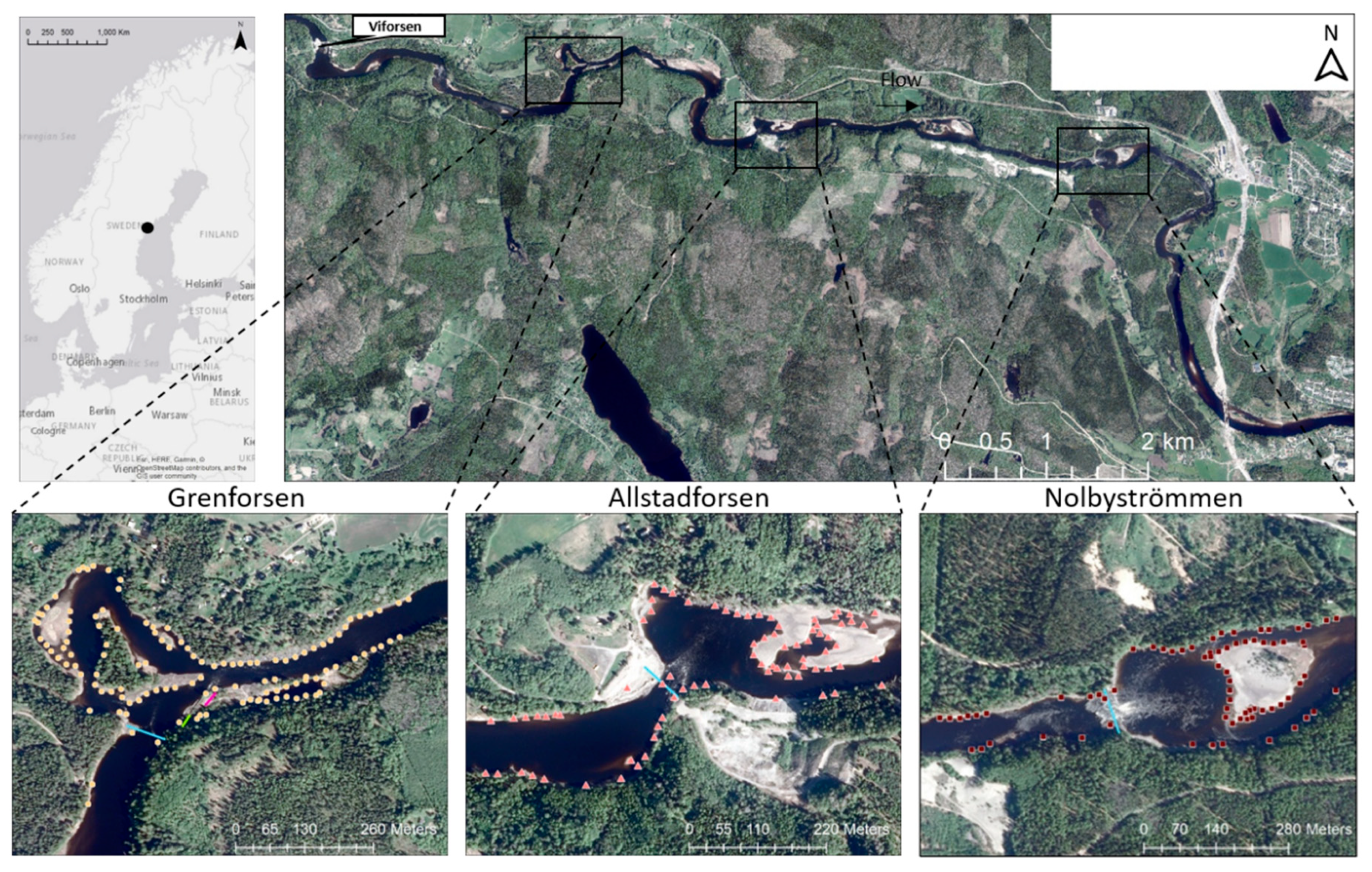
2.1. Study Area

The Ljungan River originates on the Norwegian border and runs through the middle part of Sweden before it reaches the Gulf of Bothnia. Its total length is 399 km with a catchment area of 12,851.1 km2 and a total of 15 power plants, where Viforsen power plant is the most downstream in the system (Figure 1). The instream restoration measures carried out by the stakeholders were located at three different locations: Grenforsen (Gren), Allstaforsen (Allsta) and Nolbystrommen (Nolby). The three locations were selected by the stakeholders group judged by their potential to improve the salmonid habitat quality after restoration measures were in place (Figure 1).

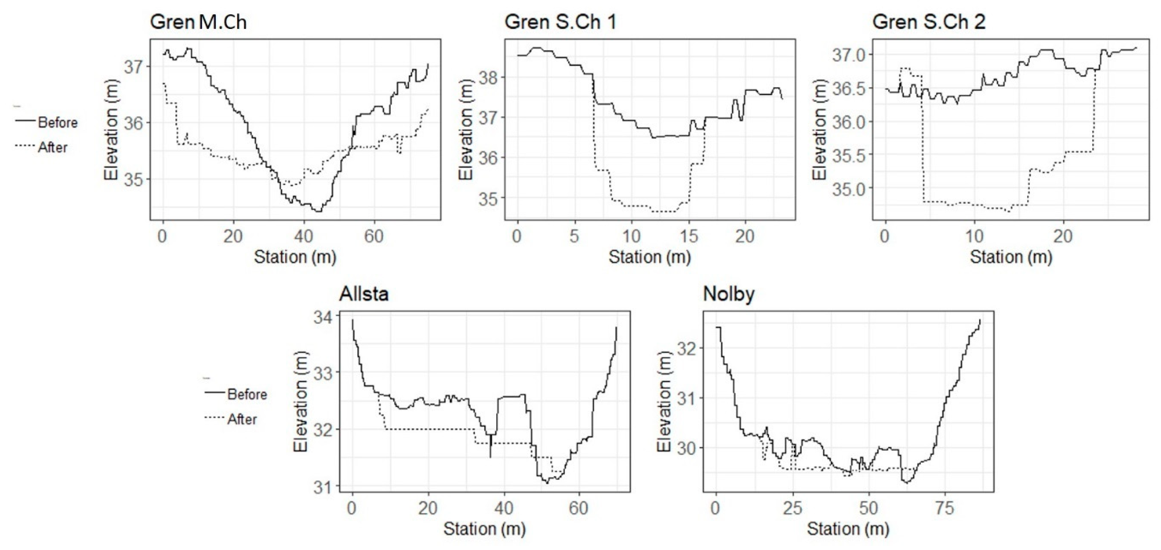
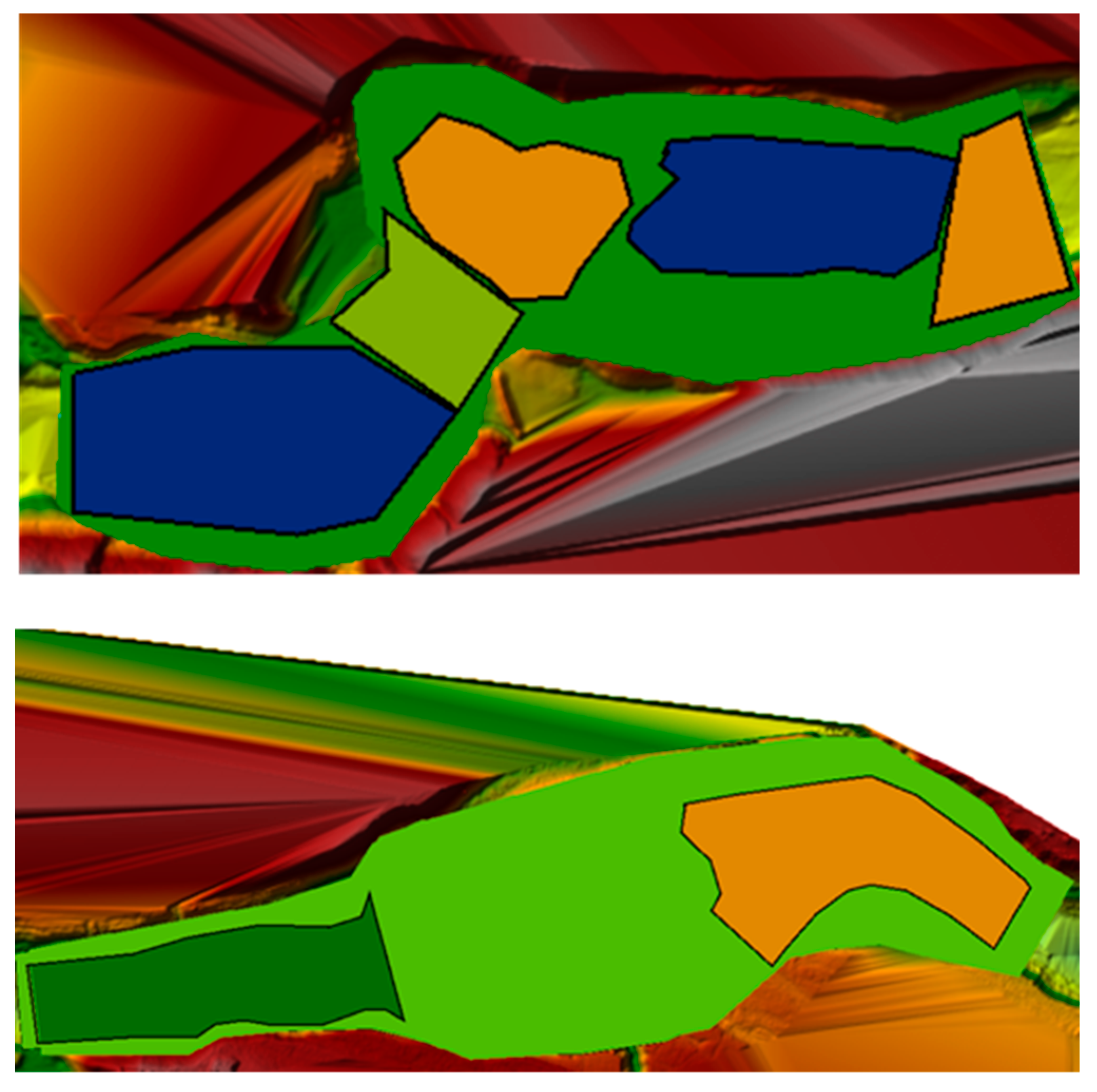
2.2. Terrain Modification

Bathymetry data were collected during an airborne LiDAR bathymetry (ALB) survey. It was conducted on 2 September 2015 by the company airborne hydro mapping (AHM), Austria, with the RIEGL VQ-880 G green laser camera [27] and lasted for 2–3 h to survey approximately 19 km. The total amount of ground points captured was 1,518,500, and it was delivered as cross sections with 5-m average distance. These ground points were already filtered by AHM who removed the raw data noise originated from the laser being scattered by birds, clouds, dust and other particles. The filtering process involved both automatic and manual filtering (see [15] for more details). In addition, vegetation was also removed from the point cloud by AHM in the pre-processing step. The survey was carried out with a measured flow of 58.9 m3 s−1 with an accuracy of 0.07 m for planar coordinates, and 0.03–0.04 m for mean vertical accuracy obtained from comparing LiDAR elevation points with manual measurements [13]. The maximum average depth reached was 2.8 m restricted by the dark bottom and organic material in the water. Therefore, additional manual data (14.190 points) were collected from the river bed and banks using a Sontek RiverSurveyor M9 acoustic Doppler profiler (ADCP) [28] equipped with a differential GPS system. The ADCP was mounted on a floating platform towed by a kayak and used to capture bathymetry points from Viforsen and 19 km downstream to the end of the area covered by LiDAR data. In addition, the ADCP was also used with a small rowing boat to survey additional points in Allstaforsen [13]. The ADCP surveys were carried out following a pre-specified route that was mapped based on the missing LiDAR data, however the precision to capture all the missing areas was subjective to the individual performance and to the external conditions, including security. In both cases, the GPS antenna system was used to capture the XY coordinates, whereas the ADCP was used to collect the bathymetric data with a sampling frequency of 1 Hz from the nine individual transducers which define the channel definition with an accuracy of 1% [28] and gives input to further development of a digital elevation model (see [13]). The LiDAR and ADCP points were combined into a point cloud used as the input to the empirical Bayesian kriging interpolation method using the average method for overlapping points in ArcGIS [29] to create a digital elevation model (DEM) with a resolution of 1 by 1 m. The DEM obtained was representative of the situation before the instream modifications were carried out. In order to simulate the situation after the modifications, a second DEM was created including the terrain modifications (Figure 2). These modifications were modelled by altering the DEM using ArcGIS and the raster editor (ArcMap Raster Edit) which allows changing the values of specific points in a raster. Three reaches in Ljungan river were modelled: Gren, Allsta and Nolby (Table 1). Two main measures were simulated: (a) Stones and rocks were moved from the banks to the main channel in Gren, Allsta, and Nolby and (b) a concrete wall was broken to open two channels: Gren S.Ch 1 and Gren S.Ch 2 (Figure 2).

2.3. Hydraulic Modeling

A two-dimensional hydraulic model with cell size of 1 by 1 m was developed for each of the three locations using the HEC-RAS 5.0 software developed by US Army Corps of Engineers [30]. The model before the restoration measures (reference model) was calibrated for a discharge of 58.9 m3 s−1 corresponding to the discharge measured during the ALB survey. The difference between the water surface elevation simulated and the values delivered by AHM based on the LiDAR data were used for the calibration. In order to validate the situation after the modifications, a simulation was done for the observed discharge on aerial pictures (65.4 m3 s−1), and the wetted area extent from the simulation results and the water edge from the aerial picture from 2017 when the instream modifications were already in place were visually compared. The successful of the instream measures were considered under the premises that the wetted area results will be as expected under the objectives (Table 1) and in addition they will match the water covered area extent after the modifications from the aerial picture provided by Lantmäteriet (www.lantmateriet.se) with 0.25 m planar resolution.
The discharges used for the hydraulic simulations before and after instream modifications were selected based on the following criteria: discharges that are dominant during the spawning season (60 m3 s−1 and 100 m3 s−1), 138 m3 s−1 is the average flow in Ljungan and 380 m3 s−1 is the average one-day maximum discharge (Table 2). In addition, because in Gren one of the measures was designed to reconnect the side channel with the main channel also on lower flows, low discharges that could be observed particularly during summer months were also analyzed. In order to provide a detailed coverage of low discharges and due to wetted area changes in a more pronounced way at low flows changes, four discharges were selected: 20 m3 s−1, 30 m3 s−1, 35 m3 s−1, and 40 m3 s−1. These discharges were used as inputs for the upper boundary condition. In addition to the 1 by 1 m cells, break lines were included in areas were higher resolution was needed (such as along river banks, islands and side channels). Crowder and Diplas [9] showed the importance of analyzing effects at a finer scale, such as the close surrounding area after placing boulders in the river. Forcing the break lines in the mesh produced a mesh with different dimensions. Normal depth was specified for the lower boundary condition, the average channel slope at the downstream part of the reach was used as an approximation of the friction slope. For the river bed roughness, Manning’s n coefficients ranged from n = 0.03 (channel with gravels and cobbles) to n = 0.15 (channel with bushes and higher resistance) [31].

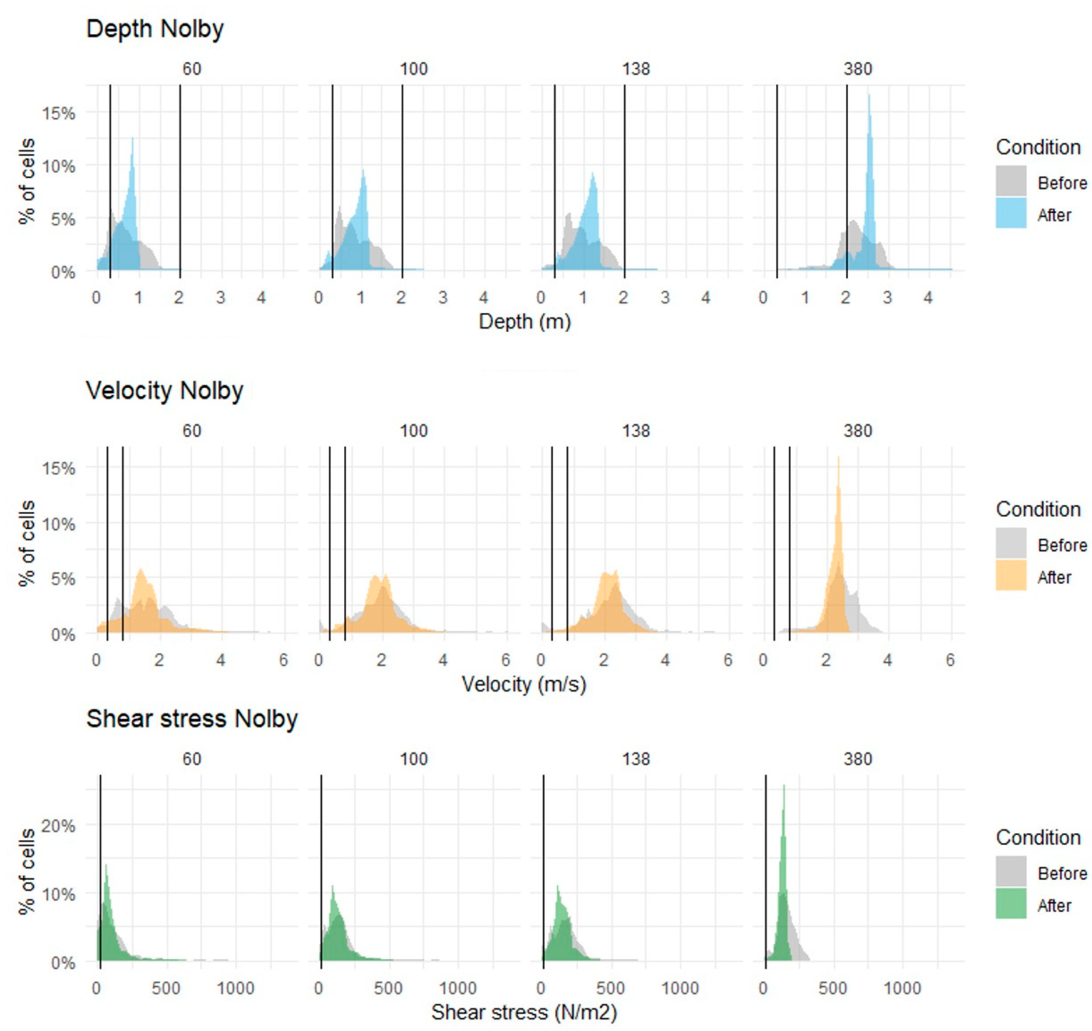
2.4. Depth, Velocity and Shear Stress Distribution and Potential Suitable Area

Water-surface elevation, depth, velocity and shear stress values were extracted as average point values for each cell in the mesh for discharges ranging from 20 m3 s−1 to 380 m3 s−1 (Table 2) before and after the modifications. An initial comparison for the situation before and after modification for the full range of parameters (depth, velocity and shear stress) was carried out. Analyses of the potential suitable area (PSA) were carried out using literature data on preferred ranges of habitat for juvenile Atlantic salmon [2,32] and available physical habitat data (spawning areas location, substrate composition, shelter distribution) that were surveyed and mapped by Uni Research in 2014 in Ljungan [33]. Physical habitat data from field measurements were used to compare and support the data obtained from literature [2,32]. The average depths and velocities simulated from the hydraulic model were exported to GIS tools and extracted at the spawning locations [33] under the average spawning discharge conditions. The same was carried out for the nursery areas. After obtaining the simulated average depths and velocities in the studied areas, the data were compared to the ones obtained from literature. This comparison showed that the simulated values agreed with the ranges from literature, except for spawning area depths. Simulated values in Ljungan river could go up to 2 m, in contrast to the values from Armstrong and Kemp [2] and Forseth and Harby [32], which did not exceed 1.5 m. Therefore, the depth range used to identify the potential suitable area was increased accordingly. PSA was calculated as the number of square meters for depth, velocity and shear stress values that fell inside the range considered suitable (Table 3). PSA was also calculated and related to the total wetted area to obtain the percentage of PSA (PSA%). Considering the uncertainties related to habitat results from the hydraulic model and in addition the lack of detailed and observed depth, velocities and critical shear stress values in the field, the analyses of the PSA were considered separately as suggested by Scruton et al. [34]. Therefore, PSA were calculated for depth, velocity and critical shear stress individually instead of weighting and summing them into an overall PSA. Critical shear stress was included under the assumption that sediment mobility for a given particle size occurs when the bed shear stress exceeds the critical shear stress [35]. Values were selected according to the predominant substrate type in the areas [33].

2.5. Calculation of Costs Per Unit of Potential Suitable Area

The cost of the modifications at each location were obtained from the project budget (Table 4). The total cost at each site was used to calculate the cost to create a unit of potential suitable area. This was used to compare the cost and the potential effectiveness of the modifications within sites and within the type of habitat created based on depth, velocity and shear stress values.

3. Results

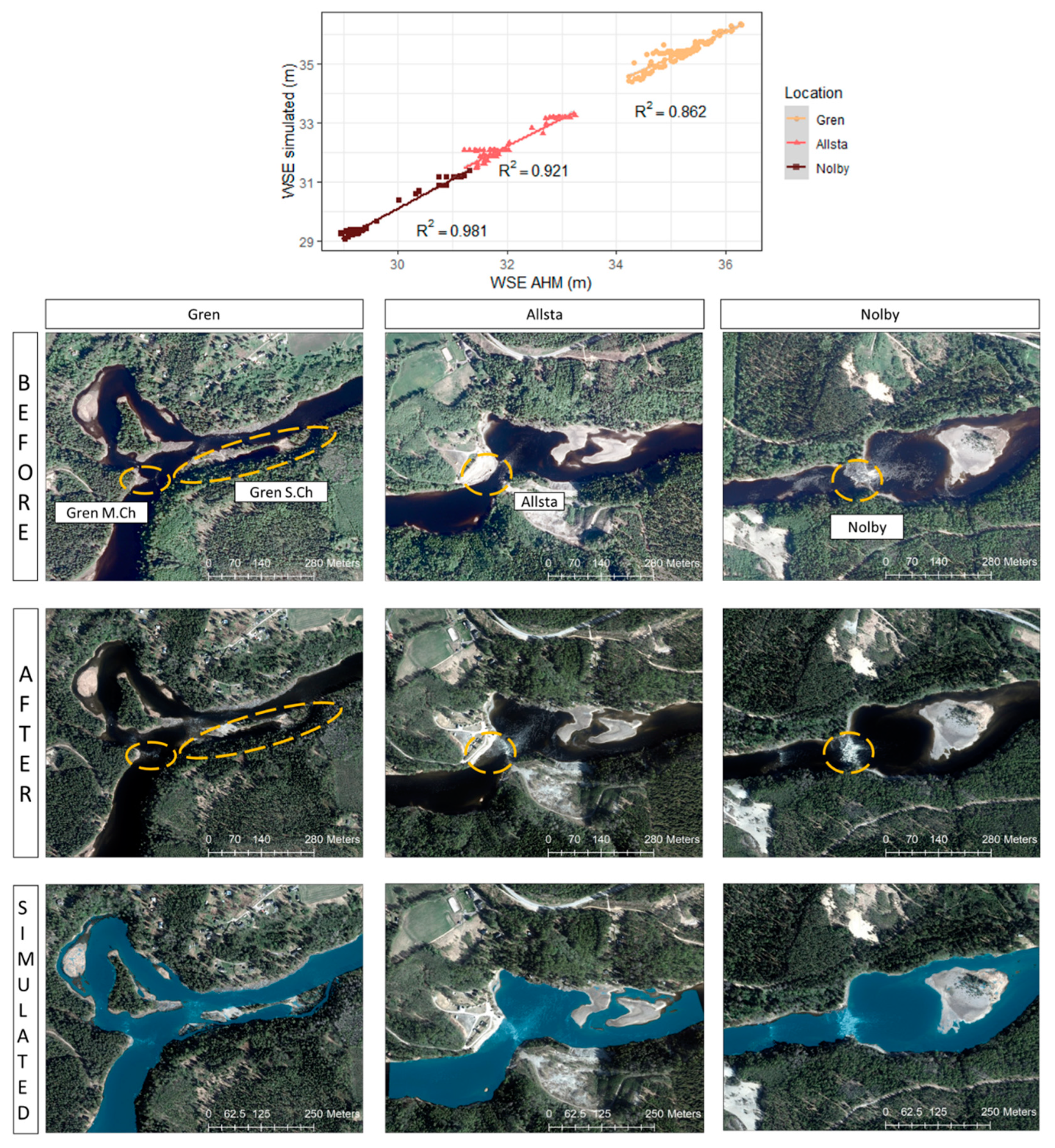
3.1. Calibration & Verification

Calibration for the situation before modifications was considered good when the correlation between the observed water surface elevation and simulated water surface elevation exceeded 0.85 (R2 ≥ 0.85). After modification, the verification was considered good when water surface extent from the simulated results matched the situation observed from aerial pictures (Figure 3). Based on the results from calibration, the hydraulic model setup for both the before and after situation were considered adequate for simulating the effects from habitat modification on depth, velocities and shear stress.

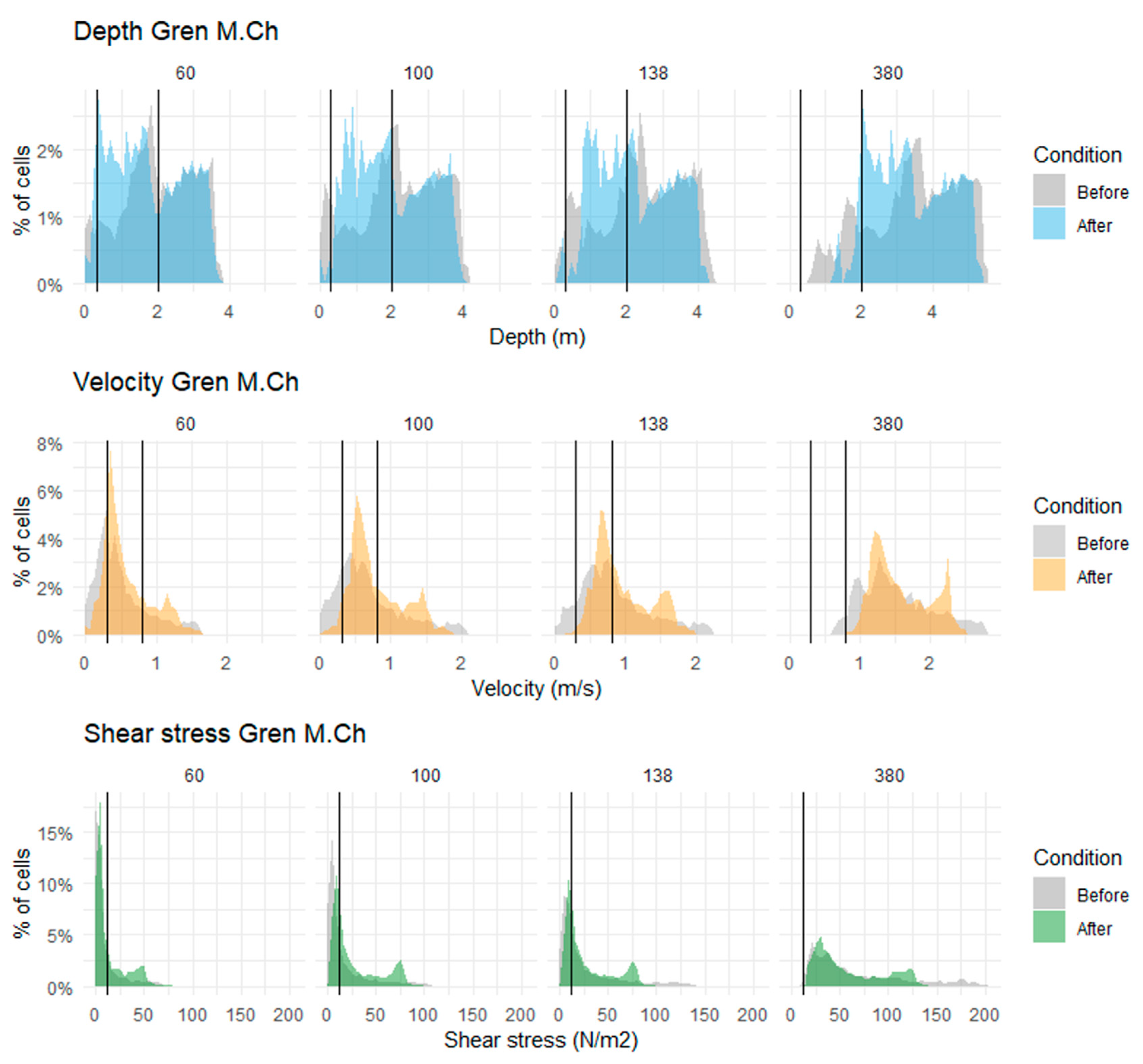
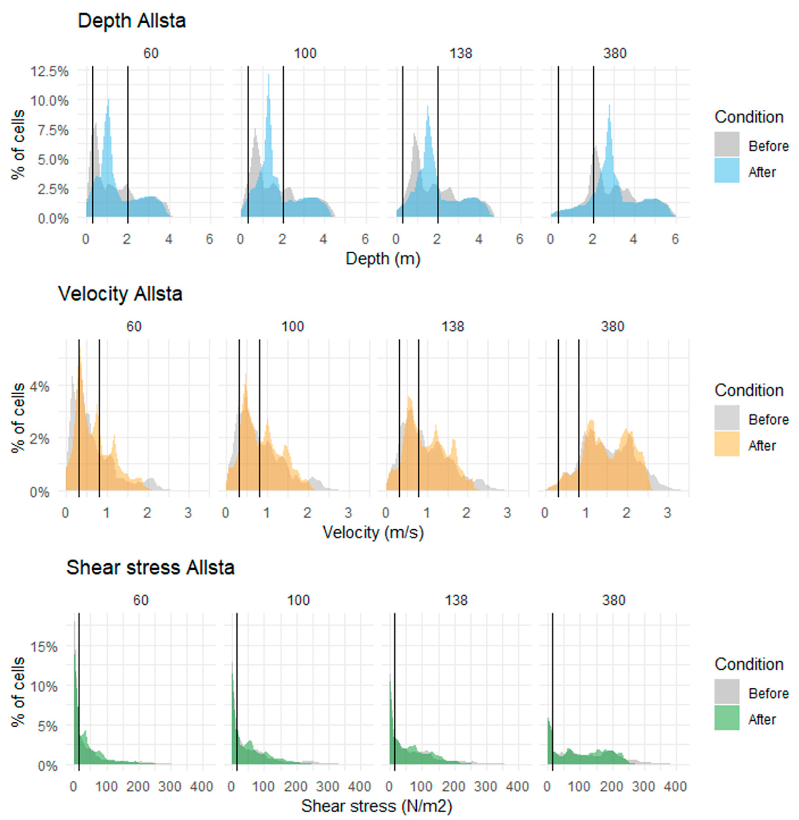
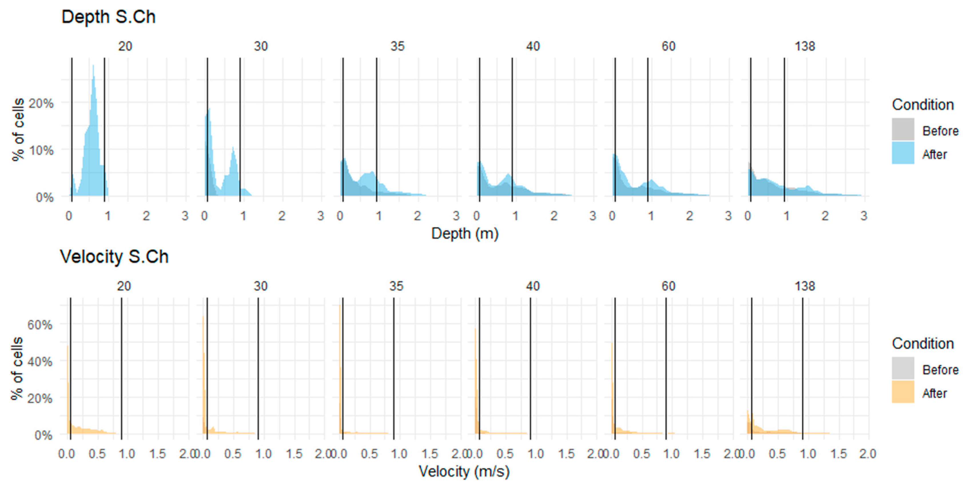
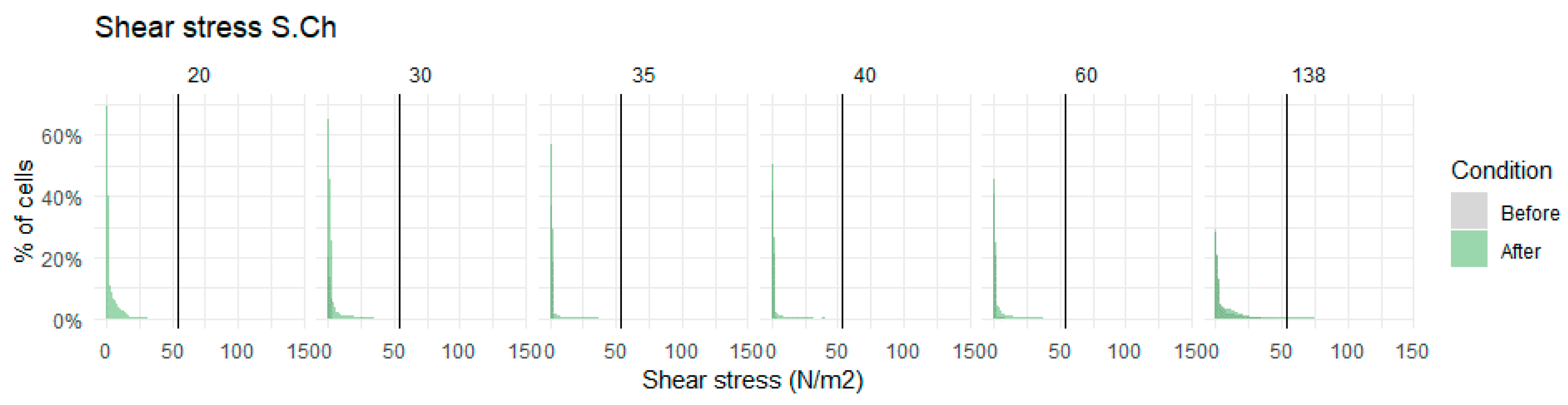
3.2. Depth, Velocity and Shear Stress Distribution

After modifications, the range of distributions for depth, velocity and shear stress was reduced. The lower values found before the modification increased after the modifications, and the higher values were reduced. This was found at Gren. M.Ch (Figure 4), Allsta (Figure 5) and Nolby (Appendix B. In Gren S.Ch (Figure 6), results showed increased values for the three parameters after modifications.
Changes in the distribution of depth and velocity, in relation to the range of potential suitable area (vertical lines) showed that the percentage of cells for discharges from 60 m3 s−1 to 138 m3 s−1 inside the specified values increased at Gren M.Ch (Figure 4), but this is not the case for the high discharge at 380 m3 s−1. The same results were found for Allsta (Figure 5) and Nolby (Appendix B). Changes in shear stress values were not that significant at any location. In Gren S.Ch (Figure 6), a general increase for the percentage of cells after instream modification was found under all discharges and for the three parameters (depth, velocity and shear stress).
Wetted areas increased at all locations and with increasing discharges after the instream modifications (Figure 7). PSA% showed an increase for depth after modifications at all locations, for velocities it also improved at all locations, especially in Gren S.Ch. Shear stress PSA% values decreased after modification at all sites except in Gren S.Ch.

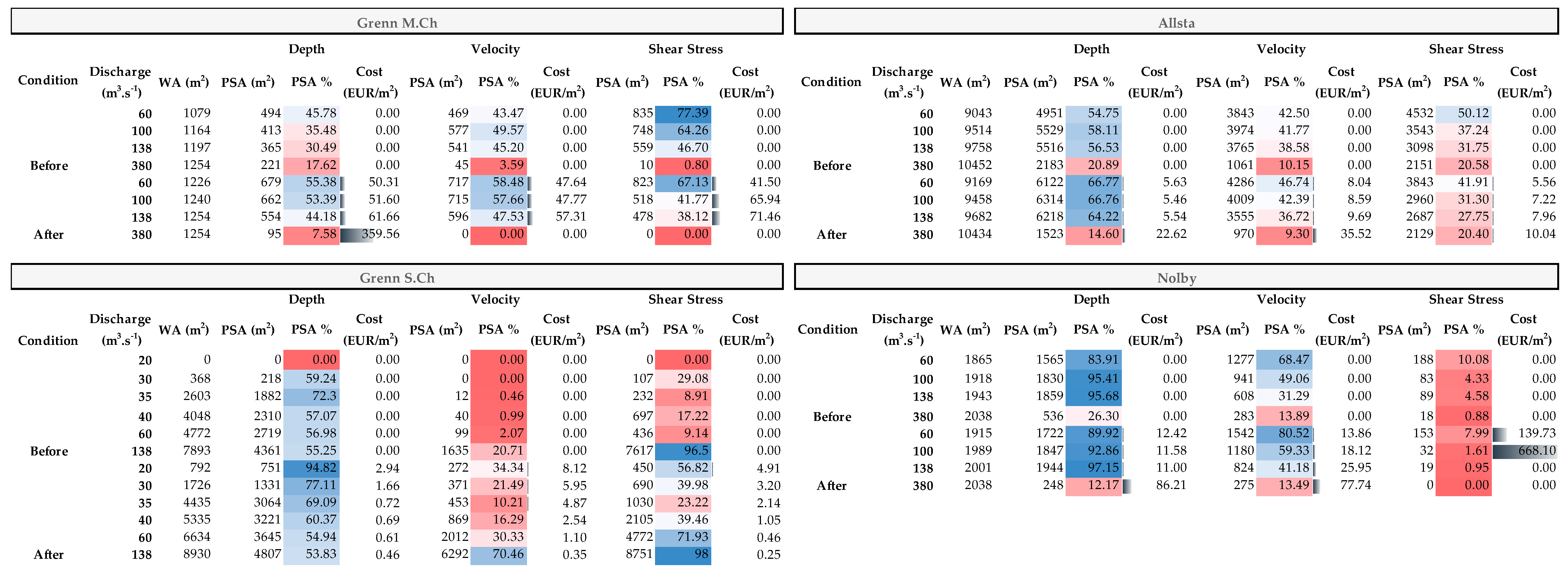
3.3. Cost Per Unit of Potential Suitable Area

The cost per unit of PSA (Figure 7) showed that the creation of PSA for depth values was the cheapest at all locations except in Grenn M.Ch, with 380 m3 s−1 as the discharge that showed the most expensive values Velocity costs showed a similar pattern as depth. Shear stress was the most expensive PSA, and Nolby exhibited the highest cost per square meter.

4. Discussion

Several concepts, tools and new techniques are used over recent decades for planning and evaluation of the feasibility of mitigation and restoration projects in rivers. The availability of high resolution bathymetry data provide the opportunity to obtain physical parameters such as depth or velocities values in a finer spatial scale distribution from 2D models compared with previous analyses carried out with 1D models, which has been reported to be more appropriate for fish habitat studies [4,9]. Despite that most of the habitat suitability studies are based on average-point depth and velocities. Pisaturo et al. [36] found that 3D modelling for habitat suitability gave significantly different results compared with 2D modelling results. This could be important if habitat suitability indexes were based on e.g., bottom flow velocity [37]. On the other hand, the 3D modelling will incur higher computational costs [38]. Based on the need for efficient computation and since we do not have the necessary fish habitat data to utilize the extra information provided by the 3D model, we decided to run a 2D simulation in this project. The 2D modelling approach has been proved to successfully simulate the water covered areas and flow patterns which is important for planning mitigation measures. The same model setup has also been shown to be efficient in evaluating the drying out areas at different flow regimes [39], which is also relevant for the study in Ljungan. This study used LiDAR bathymetry data to build a hydraulic model and analyze the depth, velocity and shear stress distributions which were used as a benchmark to evaluate the success of instream measures carried out in Ljungan river. The two types of instream measures simulated, returning stones and rocks to the river channel and opening a wall to reconnect a side channel with the main river, showed that spawning and nursery areas were potentially improved after the modifications. In addition, it also showed that Allsta was the location where the instream modification was most cost-effective. The procedure presented in this study could be used to design mitigation and restoration measures during the planning process for anticipated impacts but also in future restoration measures to improve the effectiveness aiming to improve fish habitat conditions.

4.1. Hydraulic Responses and PSA

The instream modifications aimed to improve the habitat for Atlantic salmon spawning showed an increase of water depth values and a reduction of flow velocity values comparing to the situation before modification. These findings were also observed by Gardeström et al. [40] who analyzed the abiotic effects from restoring a channelized river in Sweden, and found that after restoration, water velocities were significantly reduced and channels were wider. These effects can be related to the changes in the geomorphology, as explained by Nilsson and Lepori [25], after the reduction in the bank elevations and the return of stones and rocks to the channel, the channel structure will be more complex and so roughness and flow resistance will increase. This leads to a reduction in flow velocity and to an increase in the wetted area. Water depth could increase or decrease depending on the relative changes done in the channel. According to the values established from literature and field data [2,32] the suitable area for water depth and velocities increased at all sites for the discharges expected during the spawning season and also for the average discharge. The area showing values under the critical shear stress range chosen by literature [35] decreased after the measures at all sites. Despite values for shear stress PSA after the measures were reduced, still they exhibited a PSA% similar to the one for velocities, which was also observed for the velocity and shear stress distribution range. The same results were found by Bair [41], where the range of shear stress and velocities were reduced after large wood were placed in the river. The shear stress results and analyses for PSA presented in this study could be considered as conservative because of the following reasons: (a) Wilcock and McArdell [42] observed partial mobility of the bed to occur between critical shear stress value and twice the shear stress value, and full mobility was observed above twice the shear stress value, while the PSA in this study was calculated based just on values lower than the critical shear stress, (b) the critical value selected from literature was the minimum value indicated within a wider range for coarse gravel for the spawning area and the highest value for very coarse gravel for the nursery area, and (c) the shear stress obtained from the hydraulic model is an average value for each cell face instead of the river bed shear stress.
The instream modifications aimed to restore the nursery area reconnecting the side channel and showed increased values at Gren S.Ch for water depth, velocities and shear stress as discharge also increased. This is in agreement with Nilsson and Lepori [25], who described the predicted changes after the reconnection of cut-off side channels as increased channel area, increased total flow resistance and water volume. The largest changes were seen at lower flows, and this was expected since the channel was only disconnected under low flow conditions. At higher flows, water was still flowing into the channel from a small area with lower elevation some meters downstream of the concrete wall also before the modification. Based on the literature data to evaluate the increase in suitability nursery habitat [2,32], instream modification has led to an increase in the nursery habitat for water depth, velocity and shear stress. However, even if velocities showed an improvement after modifications the amount of potential suitable habitat created after modifications for the velocity is small compared with the amount of habitat for depth. Unlike most of the WUA studies, in this study the preferred values were considered by separate [34], however, this results may indicate that the potential suitable nursery area is not appropriate if velocities are not increased. It is also important to highlight that these values contain the uncertainties related to an inappropriate representation of the instream modification from the terrain modifications, and as for the other sites, further field data collection will be needed to corroborate these results.

4.2. Expected Ecological Responses

Several studies support that restoration measures will generally have a positive effect on fish production [43,44]. Restoration measures for spawning areas has been reported as a success by Gard [45]. They used a 2D hydraulic model and predicted an increase of WUA for salmon spawning, which was also supported by the biological monitoring data. Fjeldstad et al. [46] used 2D hydraulic modelling techniques to predict that the removal of weirs and the addition of spawning gravel would create favorable conditions for Atlantic salmon spawning, which was also corroborated with biological data. High shear stress values could cause gravel to be flushed away and consequently, salmon eggs could be scoured, however, McKean and Tonina [47] found that even at higher shear stress values a lower amount of gravel was found to be mobile at high flows. In addition, they also discussed that salmon eggs are usually buried 15–50 cm below the streambed surface, protecting the eggs to be flushed away. The reconnection of the side channel could provide suitable refuge habitat for juvenile fish [2,25]. Using a 2D hydraulic model, Koljonen et al. [48] predicted an increase in weighted usable habitat for juveniles, which was related to an observed increase of juveniles densities. However, difficult winter conditions overrode the density improvements for the next summer juveniles. Gard [45] found lower fry densities after modification than before the modifications in rearing habitats, but they suggested that their model could be used to design additional instream modifications, such as the addition of boulders and the construction of a side channel, could increase the shelter and would modify the depth and velocities values to the ones preferred by fry and juvenile salmonids. Bair [41] found an increase in the suitable habitat and shelter for salmon juveniles after large pieces of wood were added to the river bed. At the same time, shear stress values and velocity decreased. Despite these positive results, Palmer et al. [49] reported from an extensive literature review that no clear evidence for biological improvement was found after instream restorations, suggesting that a reason could be the deterioration of the habitat created after the instream measures. However, Marttila et al. [50] found that long term changes in habitat structure after restoration either remained unaltered or were reinforced through time. They were able to discard the hypothesis that the low biological improvements found after instream restoration were related to a long-term deterioration of the habitat. Therefore, based on our results for potential suitable areas and the literature findings, there are reasons to believe that future analyses of monitoring data will corroborate that the restoration measures in Ljungan improved the usable nursery and spawning areas in the river as a result of the implemented habitat adjustments.

4.3. Cost-Effectiveness

In terms of cost-effectiveness for the location of the instream measure, Allsta was the most cost-effective site where the most suitable areas were obtained for the money spent. In addition, creating suitable ranges of depth was found to be the most cost-effective measure for both spawning and nursery areas. Based on these results, Allsta and Gren S.C have shown to be the areas to prioritize for cost-effective restoration measures. However, it is important to notice that further instream works might be needed to improve the PSA for velocity values in the side channel. The term effectiveness in this study has been used to describe the effectiveness of instream measures to improve habitat conditions. However, benefits cannot be calculated until data from biological monitoring is available after the modifications in River Ljungan.
Re-stocking measures, which consist of the release of young salmon in order to compensate for the loss of habitat and migration corridors, has been carried out in many hydropower regulated rivers [51,52], but they are usually reported as a costly and ineffective mitigation measure because young salmon die in high numbers before maturing to spawning adults. [51,53] In Ljungan, re-stocking of salmon was carried out in the past, but in the last 15 years, salmon was re-stocked only in 2004 with 13,200 young salmon [54]. The cost per salmon release for re-stoking in Ljungan after bread from egg to two-year-old smolt is 2.21 EUR (21 SEK), and the costs for capture of spawning fish (trapped at Viforsen) is 16,904 EUR (160,000 SEK) per year. As an approximation, the cost for the release during 2004 could be calculated as 46,076 EUR. The total cost calculated in this study for all the instream modifications was 92,199 EUR, considering the cost over a 40-year time span at 2.5% p.a. amortization [55], the annuity cost is 3648 EUR/year. Considering the low effectiveness from the restocking measures, it is expected that instream measures will be a more cost-effective measure in Ljungan than the previous re-stocking programs. It is important to note that instream mitigation measures could require a follow-up maintenance [32], e.g., due to sediments deposited which could clog the interstitial spaces, affecting spawning and nursery areas. This maintenance measures will incur in an increment in the cost per unit of PSA that has not been included in this study. This however will be very dependent on the river and the sediment dynamics. Barlaup and Gabrielsen [44] did not find degradation of the restored spawning habitat from sediment depositions, the amount of sediments accumulated was washed away when the spawning fish built their redds. Still, Pulg et al. [56] found a degradation of the restored spawning areas from sediment deposition, expecting unsuitable areas for reproduction after five or six years. Follow-up mitigation measures could be done, among others, by harrowing the gravels using an excavator [32], or could be done addressing the sedimentation source which will require large scale river restoration [56]. Monitoring and follow up will be needed in Ljungan to determine the maintenance and cost evaluation of the degradation of spawning areas, based on initial cost elements and necessary frequency.
The suitable habitat data presented in this study is considered as a first estimation, and field data to calibrate and corroborate the results will be needed to complete the validity of the model. Biological data will make it possible to evaluate the effects from the instream restoration measures. Despite the lack of such data, this study has shown the capability to transform a cloud of bathymetry points into a user-friendly method and techniques that helps to get easily interpretable outcomes that can positively influence management decisions. It is important to highlight that the LiDAR survey was affected by turbidity and the low bottom reflection in some areas, which were supplemented by manual measurements. However, this was not the case in other rivers like Tokkeåi or Hallingdal where water conditions were clear and average depths registered were up to 5 and 6 m [13,57]. Despite this limitation, the use of LiDAR bathymetry data as inputs for the hydraulic model has shown the potential of using this type of technique to model large river reaches with high resolution and use the results to evaluate fish habitat suitability and to support cost-effectiveness mitigation and restoration measures. In this particular case, the method presented had been applied after the instream measures were carried out, but it could also support the design before its implementation, promoting that stakeholders and water managers could test alternative scenarios [58]. Therefore, a method that supports restoration measures in order to fulfill ecological and stakeholder outcomes, and that future efforts will benefit from the understanding gained, was defined by Palmer et al. [59] as the most effective restoration.

Author Contributions

K.A. and A.A.-B. conceived the idea, A.A.-B. and K.A. participated in field measurements. A.A.-B. developed the model, data analysis and wrote the manuscript, K.O. provided relevant data and information to carry out this manuscript. K.A., H.-P.F. and K.O. supervised the modelling and writing process and contributed input to analysis and presentations, and they checked and commented on the manuscript.

Funding

This work was supported by the Norwegian University of Science and Technology under a strategic scholarship awarded to the Centre of Environmental Design of Renewable Energy funded by the Norwegian Research Council.

Acknowledgments

This work was supported by Norwegian University of Science and Technology under a strategic scholarship awarded to the Centre of Environmental Design of Renewable Energy funded by the Norwegian Research Council. In addition, Statkraft AB in Sweden financially supported this study. We would like to thank Carole Rozier and Aurelie Gosset (Department of Civil and Environmental Engineering, NTNU) for their support with the modelling process and Ingrid Alne (Department of Civil and Environmental Engineering, NTNU) for collection of field measurements. Thanks to Angela Odelberg and to the rest of the members in the stakeholders group in Ljungan for their support.

Conflicts of Interest

The authors declare no conflicts of interests.

Appendix A

Figure A1. Manning areas used for the hydraulic simulations for Allsta (upper panel) and Nolby (lower panel). Blue is for areas with n = 0.03, light green n = 0.06, dark green n = 0.09, and orange n = 0.15.
Sustainability 11 01500 g0a1

Appendix B

Figure A2. Percentage of cells under values for depth, velocity and shear stress in Nolby. Vertical lines indicate the limits for the suitable range (Table 3).
Sustainability 11 01500 g0a2

References

  1. Erwin, S.O.; Jacobson, R.B.; Elliott, C.M. Quantifying habitat benefits of channel reconfigurations on a highly regulated river system, Lower Missouri River, USA. Ecol. Eng. 2017, 103, 59–75. [Google Scholar] [CrossRef]
  2. Armstrong, J.D.; Kemp, P.S.; Kennedy, G.J.A.; Ladle, M.; Milner, N.J. Habitat requirements of Atlantic salmon and brown trout in rivers and streams. Fish. Res. 2003, 62, 143–170. [Google Scholar] [CrossRef]
  3. Stamou, A.; Polydera, A.; Papadonikolaki, G.; Martínez-Capel, F.; Muñoz-Mas, R.; Papadaki, C.; Zogaris, S.; Bui, M.D.; Rutschmann, P.; Dimitriou, E. Determination of environmental flows in rivers using an integrated hydrological-hydrodynamic-habitat modelling approach. J. Environ. Manag. 2018, 209, 273–285. [Google Scholar] [CrossRef] [PubMed]
  4. Fabris, L.; Malcolm, I.A.; Buddendorf, W.B.; Millidine, K.J.; Tetzlaff, D.; Soulsby, C. Hydraulic modelling of the spatial and temporal variability in Atlantic salmon parr habitat availability in an upland stream. Sci. Total Environ. 2017, 601–602, 1046–1059. [Google Scholar] [CrossRef]
  5. Friberg, N.; Angelopoulos, N.V.; Buijse, A.D.; Cowx, I.G.; Kail, J.; Moe, T.F.; Moir, H.; O’Hare, M.T.; Verdonschot, P.F.M.; Wolter, C. Chapter Eleven—Effective River Restoration in the 21st Century: From Trial and Error to Novel Evidence-Based Approaches. In Advances in Ecological Research; Dumbrell, A.J., Kordas, R.L., Woodward, G., Eds.; Academic Press: Cambridge, MA, USA, 2016; Volume 55, pp. 535–611. [Google Scholar]
  6. Milhous, R.T.; Updike, M.A.; Schneider, D.M. Physical Habitat Simulation System Reference Manual: Version II; US Fish and Wildlife Service: Falls Church, VA, USA, 1989.
  7. Waddle, T. PHABSIM for Windows User’s Manual and Exercises; Geological Survey: Denver, CO, USA, 2001.
  8. Jay Lacey, R.W.; Millar, R.G. Reach scale hydraulic assessment of instream salmonid habitat restoration 1. JAWRA J. Am. Water Resour. Assoc. 2004, 40, 1631–1644. [Google Scholar] [CrossRef]
  9. Crowder, D.; Diplas, P. Using two-dimensional hydrodynamic models at scales of ecological importance. J. Hydrol. 2000, 230, 172–191. [Google Scholar] [CrossRef]
  10. Boavida, I.; Santos, J.M.; Cortes, R.V.; Pinheiro, A.N.; Ferreira, M.T. Assessment of instream structures for habitat improvement for two critically endangered fish species. Aquat. Ecol. 2011, 45, 113–124. [Google Scholar] [CrossRef]
  11. Mandlburger, G.; Hauer, C.; Wieser, M.; Pfeifer, N. Topo-bathymetric LiDAR for monitoring river morphodynamics and instream habitats—A case study at the Pielach River. Remote Sens. 2015, 7, 6160–6195. [Google Scholar] [CrossRef]
  12. AHM. New Possibilitiesin Bathymetricandtopographicsurvey; A. GmbH: Innsbruck, Austria, 2015. [Google Scholar]
  13. Alne, I.S. Topo-Bathymetric LiDAR for Hydraulic Modeling—Evaluation of LiDAR Data From Two Rivers; NTNU: Trondheim, Norway, 2016. [Google Scholar]
  14. McKean, J.; Nagel, D.; Tonina, D.; Bailey, P.; Wright, C.W.; Bohn, C.; Nayegandhi, A. Remote Sensing of Channels and Riparian Zones with a Narrow-Beam Aquatic-Terrestrial LIDAR. Remote Sens. 2009, 1, 1065–1096. [Google Scholar] [CrossRef] [Green Version]
  15. Andersen, M.S.; Gergely, Á.; Al-Hamdani, Z.; Steinbacher, F.; Larsen, L.R.; Ernstsen, V.B.J.H.; Sciences, E.S. Processing and performance of topobathymetric lidar data for geomorphometric and morphological classification in a high-energy tidal environment. Hydrol. Earth Syst. Sci. 2017, 21, 43–63. [Google Scholar] [CrossRef] [Green Version]
  16. Mandlburger, G.; Pfennigbauer, M.; Steinbacher, F.; Pfeifer, N. Airborne Hydrographic LiDAR Mapping–Potential of a new technique for capturing shallow water bodies. In Proceedings of the 19th International Congress on Modelling and Simulation, Perth, Australia, 12–16 December 2011; pp. 12–16. [Google Scholar]
  17. Klemas, V.; Pieterse, A. Using remote sensing to map and monitor water resources in arid and semiarid regions. In Advances in Watershed Science and Assessment; Springer: Berlin, Germany, 2015; pp. 33–60. [Google Scholar]
  18. HELCOM. Salmon and Sea Trout Populations and Rivers in the Baltic Sea—HELCOM Assessment of Salmon (Salmo salar) and Sea Trout (Salmo trutta) Populations and Habitats in Rivers Flowing to the Baltic Sea. Baltic Sea Environment Proceedings no. 126A; H. Commission: Helsinki, Finland, 2011; p. 79. [Google Scholar]
  19. Helfield, J.M.; Capon, S.J.; Nilsson, C.; Jansson, R.; Palm, D. Restoration of rivers used for timber floating: Effects on riparian plant diversity. Ecol. Appl. 2007, 17, 840–851. [Google Scholar] [CrossRef] [PubMed]
  20. Petersen Jr, R.; Madsen, B.; Wilzbach, M.; Magadza, C.; Paarlberg, A.; Kullberg, A.; Cummins, K. Stream management: Emerging global similarities. Ambio 1987, 16, 166–179. [Google Scholar]
  21. Muotka, T.; Paavola, R.; Haapala, A.; Novikmec, M.; Laasonen, P.J.B.C. Long-term recovery of stream habitat structure and benthic invertebrate communities from in-stream restoration. Biol. Conserv. 2002, 105, 243–253. [Google Scholar] [CrossRef]
  22. Törnlund, E.; Östlund, L.J.E. Floating timber in northern Sweden: The construction of floatways and transformation of rivers. Environ. Hist. 2002, 8, 85–106. [Google Scholar] [CrossRef]
  23. Johansson, U. Stream Channelization Effects on Fish Abundance and Species Composition; Department of Physics, Chemistry and Biology, Linköping universitet: Linköping, Sweden, 2013. [Google Scholar]
  24. Dudgeon, D.; Arthington, A.H.; Gessner, M.O.; Kawabata, Z.-I.; Knowler, D.J.; Lévêque, C.; Naiman, R.J.; Prieur-Richard, A.-H.; Soto, D.; Stiassny, M.L.J.; et al. Freshwater biodiversity: Importance, threats, status and conservation challenges. Biol. Rev. 2006, 81, 163–182. [Google Scholar] [CrossRef]
  25. Nilsson, C.; Lepori, F.; Malmqvist, B.; Törnlund, E.; Hjerdt, N.; Helfield, J.M.; Palm, D.; Östergren, J.; Jansson, R.; Brännäs, E.J.E. Forecasting environmental responses to restoration of rivers used as log floatways: An interdisciplinary challenge. Ecosystems 2005, 8, 779–800. [Google Scholar] [CrossRef]
  26. HELCOM. Salmon and Sea Trout Populations and Rivers in Sweden—HELCOM Assessment of Salmon (Salmo salar) and Sea Trout (Salmo trutta) Populations and Habitats in Rivers Flowing to the Baltic Sea; Balt. Sea Environ. Proc. No. 126B; H. Commission: Helsinki, Finland, 2011; p. 110. [Google Scholar]
  27. Riegl. RIEGL-VQ-880-G Data Sheet. 2014. Available online: http://www.riegl.com/uploads/tx_pxpriegldownloads/Infosheet_VQ-880-G_2016-05-23.pdf (accessed on 19 November 2018).
  28. Sontek. RiverSurveyor Specifications. 2016. Available online: http://www.quantum-hydrometrie.de/RiverSurveyor-S5-M9.pdf (accessed on 19 November 2018).
  29. ESRI. ArcGIS Release 10.5; E.S.R. Institute: Redlands, CA, USA, 2016. [Google Scholar]
  30. HEC. HEC-RAS River Analysis System Version 5.0—User Manual; Hydrologic Engineering Center: Davis, CA, USA, 2016. [Google Scholar]
  31. Chow, V.T. Open-channel hydraulics. In Open-Channel Hydraulics; McGraw-Hill: New York, NY, USA, 1959. [Google Scholar]
  32. Forseth, T.; Harby, A.; Ugedal, O.; Pulg, U.; Fjeldstad, H.-P.; Robertsen, G.; Barlaup, B.T.; Alfredsen, K.; Sundt, H.; Saltveit, S.J. Handbook for Environmental Design in Regulated Salmon Rivers; NINA: Trondheim, Norway, 2014. [Google Scholar]
  33. Skoglund, H.; Gabrielsen, S.-E.; Wiers, T. Survey of Salmon Spawning and Juvenile Habitat in River Ljungan in Sweden 2014; Uni Research Environment: Bergen, Norway, 2015. (In Norwegian) [Google Scholar]
  34. Scruton, D.A.; Heggenes, J.; Valentin, S.; Harby, A.; Bakken, T.H. Field sampling design and spatial scale in habitat–hydraulic modelling: Comparison of three models. Fish. Manag. Ecol. 1998, 5, 225–240. [Google Scholar] [CrossRef]
  35. Berenbrock, C.; Tranmer, A.W. Simulation of Flow, Sediment Transport, and Sediment Mobility of the Lower Coeur d’Alene River; U.S. Geological Survey Scientific Investigations Report 2008–5093; Geological Survey: Reston, ID, USA, 2008; p. 164.
  36. Pisaturo, G.R.; Righetti, M.; Dumbser, M.; Noack, M.; Schneider, M.; Cavedon, V. The role of 3D-hydraulics in habitat modelling of hydropeaking events. Sci. Total Environ. 2017, 575, 219–230. [Google Scholar] [CrossRef]
  37. Heggenes, J. Flexible summer habitat selection by wild, allopatric brown trout in lotic environments. Trans. Am. Fish. Soc. 2002, 131, 287–298. [Google Scholar] [CrossRef]
  38. Niayifar, A.; Oldroyd, H.J.; Lane, S.N.; Perona, P. Modeling Macroroughness Contribution to Fish Habitat Suitability Curves. Water Resour. Res. 2018, 54, 9306–9320. [Google Scholar] [CrossRef]
  39. Juárez, A.; Adeva-Bustos, A.; Alfredsen, K.; Dønnum, B.O. Performance of A Two-Dimensional Hydraulic Model for the Evaluation of Stranding Areas and Characterization of Rapid Fluctuations in Hydropeaking Rivers. Water 2019, 11, 201. [Google Scholar] [CrossRef]
  40. Gardeström, J.; Holmqvist, D.; Polvi, L.E.; Nilsson, C. Demonstration Restoration Measures in Tributaries of the Vindel River Catchment. Ecol. Soc. 2013, 18. [Google Scholar] [CrossRef] [Green Version]
  41. Bair, R. Modeling Large Wood Impacts on Stream Hydrodynamics and Juvenile Salmon Habitat; Oregon State University: Eugene, OR, USA, 2016. [Google Scholar]
  42. Wilcock, P.R.; McArdell, B.W. Surface-based fractional transport rates: Mobilization thresholds and partial transport of a sand-gravel sediment. Water Resour. Res. 1993, 29, 1297–1312. [Google Scholar] [CrossRef] [Green Version]
  43. Scruton, D.A.; Anderson, T.C.; King, L.W. Pamehac Brook: A case study of the restoration of a Newfoundland, Canada, river impacted by flow diversion for pulpwood transportation. Aquat. Conserv. Mar. Freshw. Ecosyst. 1998, 8, 145–157. [Google Scholar] [CrossRef]
  44. Barlaup, B.T.; Gabrielsen, S.E.; Skoglund, H.; Wiers, T. Addition of spawning gravel—A means to restore spawning habitat of atlantic salmon (Salmo salar L.), and Anadromous and resident brown trout (Salmo trutta L.) in regulated rivers. River Res. Appl. 2008, 24, 543–550. [Google Scholar] [CrossRef]
  45. Gard, M. Modeling changes in salmon spawning and rearing habitat associated with river channel restoration. Int. J. River Basin Manag. 2006, 4, 201–211. [Google Scholar] [CrossRef]
  46. Fjeldstad, H.P.; Barlaup, B.T.; Stickler, M.; Gabrielsen, S.E.; Alfredsen, K. Removal of weirs and the influence on physical habitat for salmonids in a norwegian river. River Res. Appl. 2012, 28, 753–763. [Google Scholar] [CrossRef]
  47. McKean, J.; Tonina, D. Bed stability in unconfined gravel bed mountain streams: With implications for salmon spawning viability in future climates. J. Geophys. Res. Earth Surf. 2013, 118, 1227–1240. [Google Scholar] [CrossRef] [Green Version]
  48. Koljonen, S.; Huusko, A.; Mäki-Petäys, A.; Louhi, P.; Muotka, T. Assessing Habitat Suitability for Juvenile Atlantic Salmon in Relation to In-Stream Restoration and Discharge Variability. Restor. Ecol. 2013, 21, 344–352. [Google Scholar] [CrossRef]
  49. Palmer, M.A.; Menninger, H.L.; Bernhardt, E. River restoration, habitat heterogeneity and biodiversity: A failure of theory or practice? Freshw. Biol. 2010, 55, 205–222. [Google Scholar] [CrossRef]
  50. Marttila, M.; Louhi, P.; Huusko, A.; Mäki-Petäys, A.; Yrjänä, T.; Muotka, T. Long-term performance of in-stream restoration measures in boreal streams. Ecohydrology 2016, 9, 280–289. [Google Scholar] [CrossRef]
  51. ICES. Summary of ICES Advice on the Exploitation of Baltic Sea fish Stocks in 2018; The Fisheries Secretariat Stockholm: Stockholm, Sweden, 2017. [Google Scholar]
  52. Johnsen, B.O.; Arnekleiv, J.V.; Asplin, L.; Barlaup, B.T.; Næsje, T.F.; Rossenland, B.O.; Saltveit, S.J.; Tvede, A. Hydropower Development- Ecological Eeffects. In Atlantic Salmon Ecology; Aas, Ø., Einum, S., Klemetsen, A., Skurdal, J., Eds.; John Wiley & Sons Ltd.: Chichester, UK, 2011. [Google Scholar]
  53. Saltveit, S.J. The effects of stocking Atlantic salmon, Salmo salar, in a Norwegian regulated river. Fish. Manag. Ecol. 2006, 13, 197–205. [Google Scholar] [CrossRef]
  54. Palmé, A.; Wennerström, L.; Guban, P.; Ryman, N.; Laikre, L. Compromising Baltic Salmon Genetic Diversity: Conservation Genetic Risks Associated with Compensatory Releases of Salmon in the Baltic Sea; Havs-och vattenmyndigheten: Göteborg, Sweden, 2012. [Google Scholar]
  55. Szałkiewicz, E.; Jusik, S.; Grygoruk, M.J.S. Status of and Perspectives on River Restoration in Europe: 310,000 Euros per Hectare of Restored River. Sustainability 2018, 10, 129. [Google Scholar] [CrossRef]
  56. Pulg, U.; Barlaup, B.T.; Sternecker, K.; Trepl, L.; Unfer, G. Restoration of spawning habitats of brown trout (Salmo trutta) in a regulated chalk stream. River Res. Appl. 2013, 29, 172–182. [Google Scholar] [CrossRef]
  57. Skeie, L. Hydrauliskc Modelling of Tokkeåi-Hydraulisk Modellering av Kraftverksdrift i Tokkeåi; NTNU: Trondheim, Norway, 2017. (In Norwegian) [Google Scholar]
  58. Kennen, J.G.; Stein, E.D.; Webb, J.A. Evaluating and managing environmental water regimes in a water-scarce and uncertain future. Freshw. Biol. 2018, 63, 733–737. [Google Scholar] [CrossRef]
  59. Palmer, M.A.; Bernhardt, E.S.; Allan, J.D.; Lake, P.S.; Alexander, G.; Brooks, S.; Carr, J.; Clayton, S.; Dahm, C.N.; Follstad Shah, J.; et al. Standards for ecologically successful river restoration. J. Appl. Ecol. 2005, 42, 208–217. [Google Scholar] [CrossRef] [Green Version]
Figure 1. Ljungan River and the three locations in which restoration measures have been carried out. Coloured lines represent cross sections explained in Section 2.3 (Figure 2). Points, triangles and squares in Grennforsen, Allstaforsen and Nolbystromen, respectively, represent the measured water edge and are used in Section 3.1 (Figure 3) to verify the hydraulic model.
Sustainability 11 01500 g001
Figure 2. Elevation along the cross sections (colored lines in Figure 1) extracted from the digital elevation model (DEM) before (solid line) and the DEM after (dashed line) habitat adjustments in the areas were modifications took place. Figure 1 shows the cross-section lines location, colors correspond to Gren M.Ch in blue, Gren S.Ch 1 in green and Gren S.Ch 2 in pink in Grenforsen. Allsta has one in blue, and in Nolbystromen, Nolby in blue.
Sustainability 11 01500 g002
Figure 3. Calibration for the hydraulic model before (upper graph) showing water surface elevation simulated (WSE simulated) against water surface elevation measured by airborne hydro mapping (WSE AHM). The three panels (lower figures) show the visual verification of the hydraulic model after modifications at Gren, Allsta and Nolby. Aerial pictures from before and after modifications and simulated water surface for three locations are presented. Blue color is the water surface extent obtained from the hydraulic model and overlap by the aerial picture after modifications. Names for the sub-locations are shown, and the areas analyzed are marked with orange circles.
Sustainability 11 01500 g003
Figure 4. Percentage of cells for values of depth, velocity and shear stress in Gren M.Ch. for the four different simulated discharges. Vertical lines indicate the limits for the suitable range (Table 3). Darker areas appear as a result of overlapping the before and after graphs.
Sustainability 11 01500 g004
Figure 5. Percentage of cells for values of depth, velocity and shear stress in Allsta for the four different simulated discharges. Vertical lines indicate the limits for the suitable range (Table 3). Darker areas appear as the result of overlapping the before and after graphs.
Sustainability 11 01500 g005
Figure 6. Percentage of cells for values of depth, velocity and shear stress in Gren S.Ch for the six different simulated discharges. Vertical lines indicate the limits for the suitable range (Table 3). Darker areas appear as the result of overlapping.
Sustainability 11 01500 g006aSustainability 11 01500 g006b
Figure 7. Wetted area (WA), potential suitable area (PSA) and potential suitable area percentage (PSA%) calculated as the percentage of PSA related to the WA (blue colors are for higher values and red for lower for (PSA%) and cost (Cost) per unit of potential suitable area (grey bars are used as a cost indicator). These are calculated for each location (grey rectangle), for depth, velocity and shear stress values under the discharges evaluated. When PSA was 0, costs has not been considered.
Sustainability 11 01500 g007
Table 1. Name for the six scenarios simulated at the three locations, their status before and after modifications and the objective to fulfill after the modifications.
LocationSub LocationBefore ModificationsAfter ModificationsObjective
GrenGren M.ChNarrow channel with high banksWider channel, rocks that were on the banks were placed in the middle. Gravel and cobbles were added.Reduce water velocities, increase the wetted area and create suitable habitat for spawning.
Gren S.ChConcrete wall was blocking water to flow in the right-side channel under low flowsWall was opened in two channels (Gren. S.Ch 1 & Gren. S.Ch 2) so water could flow inside the right-side channel, even at low flowsRestore the right-side channel and its function as a nursery area as well as to restore connectivity.
AllstaNarrow channel with higher elevations in the banksWider channel, rocks that were on the banks were placed in the middle. Gravel and cobbles are added.Reduce water velocities, increase the wetted area and create suitable habitat for spawning.
Nolby Narrow channel with higher elevations specially in the right-side bankWider channel, rocks that were on the right-side banks were placed in the middle. Gravel and cobbles are added.Reduce water velocities, increase the wetted area and create suitable habitat for spawning.
Table 2. Parameters used for the hydraulic simulations in each reach.
ReachDischarge (m3 s−1)# of CellsDimensions (m2)Normal Depth (m)Manning’s 1
Gren20, 30, 35, 40, 60, 100, 138, 380364.436Max: 1.92 m2
Min: 0.01 m2
Avg: 0.90 m2
0.010.06
Allsta60, 100, 138, 380147.229Max: 1.73 m2
Min: 0.34 m2
Avg: 0.99 m2
0.0010.03, 0.06, 0.15
Nolby223.121Max: 1.74 m2
Min: 0.05 m2
Avg: 0.93 m2
0.0010.06, 0.08, 0.15
Table 3. Values used to determine the potential suitable area based on literature data [2,32] and field data [33].
Spawning AreaNursery Area
Depth (m)0.3–2.0 0.05–0.9
Water velocity (m s−1)0.3–0.80.06–0.9
Critical shear Stress (N/m2)12.253.8
Table 4. Costs in EUR per location and action. Values were converted from Swedish Kroner to Euro using the annual average exchange rate for 2016 (0.105653917).
ExcavatorHelicopterGravel
1–10 cm
Cobbles
10–100 cm
Coarse Cobbles
50–100 cm
Total
Gren M.Ch220824,08965510131034,158
Gren S.Ch220800002208
Allsta250424,08965510131034,454
Nolby 540412,0453275065521,379
Total12,32460,22316,3760327592,199

