The Impact of Employment Self-Sufficiency Measures on Commuting Time: Case Study of Perth, Australia

Abstract

The level of commuting in cities is an important indicator of the efficiency of urban spatial structure. Recent research has come out in support of land use policies that promote balancing the number of employment opportunities and residents in local geographical units to reduce excess commuting. This study explores three employment self-sufficiency indices: job-worker balance (JWB), employment self-sufficiency (ESS) and employment self-containment (ESC), as measures for reducing the level of commuting. Using the case of Perth, Western Australia, we perform a trip-based evaluation of these three variables and investigate their effect on commuting time through statistical correlation. The results reveal that JWB, ESS and ESC levels are relatively poor across the metropolitan region. Higher ESS correlates with lower inflow travel time, but better JWB and higher ESC do not necessarily lead to shorter travel times. The findings of this study suggest that policies solely relying on these measures may not be effective in reducing commuting times. ESS and ESC do not account for the component of the trip outside the zone, which can misrepresent the level of commuting in an area. Incorporating travel time in these measures can complement their reliability, and better represent overall commuting levels within an urban structure.

1. Introduction

The traditional city structures were monocentric, with jobs located in the central prime land and residences in the suburbs. As cities got bigger, efforts were directed towards decentralising jobs and bringing them closer to the people as a way to reduce the level of commuting and its related problems. Studies have reported a steady migration of jobs to the suburbs over the past several decades [1]. These developments have changed the conventional city structure, shifting it from the traditional monocentric structure towards some degree of polycentricity. As a result, many suburbs are no longer just dormitories for centrally located jobs but have become destinations in their own right.

Despite these efforts, and material changes thereof, studies have shown that commuting distances have continued to get longer in many cities [1]. Additionally, traffic congestion has reached unprecedented levels in major metropolitan areas. Newman and Kenworthy [2] and Cervero [1] contend that part of the reason is the existence of job-worker imbalances at sub-regional level within metropolitan areas. They argue that despite the decentralisation, more people now live farther from their jobs [1,3]. This shows that balance does not necessarily result in people working near to where they live. While it is reasonable to expect that increasing job opportunities nearby will increase the chances of people working nearby, there is a complex range of factors at play, including skills match and housing affordability among others.

There has been a growing research interest towards unraveling urban mobility, and developing methodologies for measuring it. Recent research efforts have ranged from urban data preparation and improvement [4,5] to the development of new indices and models for understanding urban movements [6,7]. The advances in big data analytics are also enabling researchers to examine the complex patterns of urban mobility such as temporal trends in trips to various destinations within cities (e.g., see Zhao, Chinnasamy [8]). Some researchers have taken the perspective of accessibility, evaluating access equity across cities through specific travel time thresholds for jobs and other urban services [9,10]. Others have aligned with the notion of a job-worker balance and suggested more nuanced measures which take into account the skills match between jobs and workers. Beyond the numerical balance, research interest is increasingly moving towards self-sufficiency (maximising local employment opportunities) and self-containment (maximising local capture of the labour force) within sub-regional units of major cities [11,12].

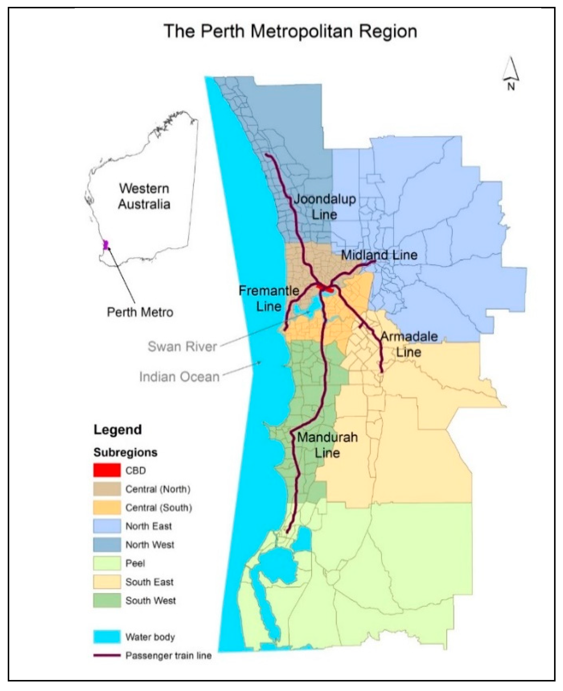
In Australia, over 60% of the population lives in the five largest cities. These cities are also experiencing the most growth in population and travel demands. Perth, the Western Australian capital, had the highest population growth rate since 2004, at 30 per cent [13]. Most of this growth occurred at and beyond the fringes [14,15] with no corresponding job supply to complement it [16]. The Perth central business district (CBD) and its surrounds remain the biggest centre of employment, with around 20% of the Perth metropolitan total. The high number of commuters from around the metropolitan region to the CBD creates unpleasant traffic conditions during peak hours. In response, the current policy objective seeks to curb urban expansion, create more suburban jobs at decentralised activity centres, and encourage local employment to reduce the long commutes [15,17].

Since the 1950s, Perth’s strategic plans have advocated balanced regional growth and job distribution to reduce the impact of commuting [12,18]. The Australian “suburban dream” and the associated higher car ownership levels have consistently led to an increase in commuting between the CBD and the suburbs. According to Martinus and Biermann [19] “commuting has continued to challenge the liveability and infrastructure efficiency of Perth and Peel” (p. 1). In parallel to the academic literature [20,21,22,23], recent strategic plans, such as Direction 2031 and Perth and [email protected] Million, have also emphasized employment self-sufficiency and self-containment as tools to determine the equity of job distribution and the reduction in commuting flows [15].

While a significant body of literature expounds upon job-worker balance (JWB), less attention has been given to self-sufficiency and self-containment. Moreover, the effectiveness of these measures in reducing commuting within metropolitan areas remains largely untested and contentious. Previous studies by Biermann and Martinus [11] and Martinus and Biermann [12] have examined these policy targets and suggested strategies by which they might be achieved in the Perth sub-regions. The former study explored three employment targets of self-sufficiency, self-containment and the job-housing balance with particular focus on Perth’s Central and North West sub-regions. The latter explored employment self-containment in the North West sub-region by performing a nuanced disaggregation of commute data by industry and occupation. These studies provide great insight into the [relationship between] employment and commuting patterns in general, and in Perth’s North West sub-region in particular. However, there remains a need to understand commuting patterns in the metro region as a whole, and how they relate to each of the three different employment self-sufficiency measures mentioned above. This study sought to empirically test the effectiveness of job-worker balance (JWB), employment self-sufficiency (ESS) and employment self-containment (ESC) using the case study of Perth Metropolitan Region (PMR), Australia. We investigate both the levels and spatial patterns of JWB, ESS, and ESC using trip data. We then compare the results with the modelled average travel times in the region to test their statistical correlations.

In the next section we present a discussion of existing literature on this subject, followed by a description of the methods engaged in the study. We then present the results of the study, which are followed by a section of their discussion, and finally the conclusion.

2. Literature Review

2.1. Defining Job-Worker Balance and/or Job-Housing Balance

The idea of co-locating jobs and housing units is not new; it goes as far back as 1898 to the utopian idea of a ‘Garden City’ envisioned by Ebenezer Howard [24]. Margolis [25] was the first to translate job-housing balance (JHB) as a concept into planning practice [26]. JHB is defined as “the distribution of employment relative to the distribution of workers in a given geographic area” [27] (p. 305). In this definition housing is taken to represent workers—their population and/or distribution. While some studies have used household data (e.g., Zhao, Lu [28] and Li and Liu [29]), many directly use worker or trip (journey-to-work) data, with a focus on commuting patterns, and attach little reference to housing (e.g., Cervero [1]; Giuliano and Small [30,31,32,33]). The job-housing balance, therefore, is a perpetuated misnomer for a concept that is more appropriately termed job-worker balance. Nonetheless, the term job-worker balance is much less used in the literature. It is noted that studies in the field of urban planning tend to use housing or household data while those in the transport field often use worker and trip data [26]. Giuliano [27] rightly observes that “the central concern of jobs-housing balance as it relates to transportation policy is the journey to work” (p. 305). Using household-based data to draw transport implications is susceptible to gross errors emanating from the variation in household structures/sizes and participation in the labour force.

2.2. Benefits and Challenges of Achieving Job-Worker Balance

The argument for job-worker balance is based on the premise of reducing the distances of commuter trips, and consequently reducing traffic congestion and improving overall traffic conditions. Previous studies have found that a better balance between jobs and workers results in reduced average commuting distances and times [23,34,35]. Moreover, decentralising jobs to achieve a balance between the number of local jobs and worker residences increases job opportunities near the people, and many are inclined to take that opportunity to minimize disutility [33]. This also encourages the use of active modes (e.g., walking and cycling) as proximity to work lessens the need for motorized vehicles [36]. Shorter commuting distances and less car dependence can have several environmental and health benefits such as less air pollution and an improved quality of life [35]. Cervero [1] also noted that a localised parity between jobs and workers might create localised commuter traffic zones segregated from regional traffic, thus easing the pressure on regional traffic streams.

In the ongoing discussion of job-worker balance, a controversial issue has been whether it is the appropriate approach to transportation problems. While the good intentions of job-worker balance are undisputed, arguments against its suitability have ranged from a wrongly premised misdiagnosis of the commuting problems, to those which are outright infeasible. One study that has received a lot of attention, by Giuliano [27], critically investigated this issue and concluded that job-worker balance is not an effective solution to ameliorate commuting and associated challenges. Quigley [37] indicates that a complex range of factors influence residential location choices, including quality of neighbourhood, quality of schools, amenities and racial mix, which makes JWB an infeasible target.

Even those who advocate balance also admit that it does not suffice as a solution. Cervero [38] states that “jobs-housing ratio only indicates the potential for balance” (p. 12). Also, its relationship with self-containment has been found to be weak [39], meaning that living close to jobs does not necessarily result in people working locally (job/skill mismatches). A proper functional balance can be realised by promoting two local community objectives that are less vague and more direct; maximising local capture of the labour force, termed “self-containment”, and maximising local employment opportunities, termed “self-sufficiency” [40]. Self-containment measures the proportion of residents that work locally, and self-sufficiency measures the proportion of jobs filled by residents [11]. Over and above a numerical parity, self-sufficiency and self-containment promote spatial ‘matches’ between jobs and workers, which can bring down commuting times. However, the impact of self-sufficiency and self-containment on commuting time has rarely been examined.

2.3. Measuring Job-Worker Balance (JWB)

The measurement of JWB is generally classified into two categories. The first one compares the number of jobs and housing units in a given area. This approach uses housing units as a proxy for workers, to circumvent data limitations. The rule of thumb is to set a threshold range that constitutes a balance, e.g., if the jobs-housing ratio lies between 0.75 and 1.25 [25]. Anything outside this range is considered ‘unbalanced’, with the lower end of the range indicating residence dominance, and the higher end indicating job dominance. When taking into account households with two or more workers, fewer houses may be needed and the threshold ceiling may be brought up [1]. Alternatively, and perhaps more accurately, actual worker numbers may be used instead of residential dwelling units. Each worker is assumed to have one job; hence a much smaller ‘balance’ range is appropriate.

The second approach seeks a balance between ‘matching’ jobs and workers, i.e., workers should live in the same area as their workplace. While the former approach only evaluates the ‘potential’ for balance, this one determines the actual balance in a locality. Thus, it can also give an indication of the match between jobs and skills in the labour force, housing affordability for local workers, or the interest of workers pertaining to living in the area [40]. With this approach we are also able to determine the level of inter-regional commuting. It therefore enables us to evaluate the levels of local employment–self-sufficiency–and the local capture of employment—self-containment [11,40]. Employment self-sufficiency indicates the level of inward commuting and employment self-containment indicates the level of outward commuting. When there is no inward commuting, the area is considered to be fully self-sufficient, and no outward commuting signifies full self-containment [11].

2.4. The Link between JWB and Commuting Behavior

There prevails a long-standing debate in the literature on city spatial structure and how/whether it affects commuting patterns, or even travel behaviour in general. Some scholars have argued that spatial structure has little if any effect on commuting patterns, and policies based on this link are wasteful and futile [27,30,41]. Peng [42] contends that vehicle-miles travelled (VMT) is only marginally linked to changes in job-housing ratios. In his study, Peng demonstrates that VMT responds to JWB only in extremely imbalanced (very job-rich or very job-poor) areas. He therefore concludes that since most areas are roughly balanced, policies targeting JWB will only affect a small portion of the city, and thus have very little impact on overall commuting in the region.

A number of studies have highlighted the relationship between proximity to jobs and commuting time. For example, Cervero [1] found that the job-housing balance was significantly inversely related to commuting time in 40 major suburban employments centres in the United States. Another study by Zhao, Lu & Linden [28] also found a significant negative relationship between home-based job proximity and mean commuting time in Beijing (China). The same study revealed that job proximity could explain an overwhelming 68% of the commuting time changes. An increasing number of studies over the past three decades have reiterated not only the existence of this relationship, but also the necessity of its uptake into land use planning policies [2,24,31,33,43,44,45]. These studies attest and contribute to the value of co-located and/or proximate jobs and residences in reducing average commuting times, as well as address other important issues including congestion, efficiency and sustainability within metropolitan settings.

Similarly, an increasing number of planning authorities in cities around the world are incorporating job-worker ratio targets in their land-use policies. Many cities around the world, in both developed and developing countries, are in a desperate pursuit of congestion solutions. Since congestion happens during the peak times when people are commuting to/from work [46], it is reasonable to expect that better balances of job-worker ratios in local sub-regions would create the potential for reduced overall commuting. With better ESS and ESC (which maximize local job opportunities and local labour capture, respectively), this potential for balance can be realised.

3. Materials and Methods

3.1. Study Area

Perth is the capital city of Western Australia, which is the biggest state in the country (about a third of the total) by land mass. Apart from escarpments to the East and some areas of shallow ground water, little stands in the way of the city’s expansion. On the north-south dimension, the Perth metropolitan region (PMR) spans over 100km of the coast, and the city’s longest train lines follow the land expansion in this direction. Altogether, Perth has five passenger train lines which all terminate at the city centre; Joondalup Line, Mandurah Line, Fremantle Line, Midland Line and Armadale Line. Figure 1 shows the geographical location of PMR. The subdivisions within the PRM represent the Strategic Transport Evaluation Model (STEM) zones, on which the analysis is based.

3.2. Data

This study used trip data generated from the STEM. STEM is a macroscopic/strategic level multi-modal model of Perth’s land use and transport systems held by the Department of Transport. The model was developed based on trip data from the 2006 Perth and Regions Travel Survey, but has been updated to 2011 using the census journey-to-work data collected by the Australian Bureau of Statistics [47]. It divides the metro region into 472 zones, and estimates the number of trips between these zones for various purposes (work, education, shopping) and by different travel modes. Model outputs include average travel times by public transport and by car for four time periods: AM peak, daytime between the peaks, PM peak and evening/night-time. In this study, we focus on home-based work trips and aggregate flows by all travel modes, since the interest is on relations between job and residence locations. Since the model data does not have walking and cycling travel times between zones, we estimated these based on the road network.

3.3. Indices for Job-Worker Balance (JWB), Employment Self-Sufficiency and Employment Self-Containment (ESC)

We have used the work trip data to define and measure indices for JWB, ESS and ESC. Our JWB index is a refinement of the conventional JHB index, based on actual home-based work trips committed. Trip origins represent residences while destinations represent jobs. JWB is therefore defined as the total of inflow trips from other zones within the PMR to a target zone, and intrazonal (internal) trips within the target zone divided by the number of outflow trips from the targeted zone to other zones in PMR, and intrazonal trips within the target zone (see Equation (1)). The numerator represents the number of jobs in the target zone (occupied by both residents and non-residents), while the denominator is the total workers living in that area.

$$JW{B}_i=\frac{{\displaystyle \sum _j^{n}inflo{w}_{ji}+intr{a}_i}}{{\displaystyle \sum _j^{n}outflo{w}_{ij}+intr{a}_i}}$$

(1)

where, JWB_i represents the job-worker balance index of zone i, inflow_ji is the number of incoming work trips from zone j to zone i, n is the number of zones in PMR except the zone i, intra_i is the number of work trips within zone i, and outflow_ij is the number of outgoing trips from zone i to zone j.

A JWB index of more than 1 means the zone is job-dominated, i.e., more inflow of work trips than outflow. An index of less than 1 means the zone is residence-dominated, i.e., more outflow of work trips. An index of 1 is balanced. In this study, we consider values between 0.8 and 1.2 to denote a balance of jobs and workers in a zone, less than 0.8 means residential dominance and more than 1.2, job dominance.

In addition to comparing the numerical balance between jobs and resident workers, we are also interested in understanding the match between local jobs and resident workers. Inter-zonal commuting is inherently a factor of the proportion of local jobs filled by local residents (Equation (2)), and the proportion of resident workers who work in local jobs (Equation (3)).

$$ES{S}_i=\frac{intr{a}_i}{{\sum }_j^{n}inflo{w}_{ji}+intr{a}_i}$$

(2)

$$ES{C}_i=\frac{intr{a}_i}{{\displaystyle \sum _j^{n}outflo{w}_{ij}}+intr{a}_i}$$

(3)

ESS indicates the level of inward travel, and the higher the ESS ratio the less travel into the area, e.g., an ESS measure of 85% means that 15% of local jobs are filled by non-resident workers who then have to commute into the area. ESC indicates the level of outward travel, and a high ratio of ESC means fewer people have to travel out of the local area for work [11]. ESC can also be alternatively defined as the proportion of internal trips to the total trips made by residents of a particular locality [39,48]. For those zones in which reducing outward travel is the objective, ESC is an appropriate index to measure their performance.

For analysis in this study, we used Geographic Information Systems (GIS) aggregation tools to determine the number of intra, inflow and outflow trips for each zone and visualized JWB, ESS and ESC using thematic mapping methods. We also analysed spatial and statistical relationships between travel time and JWB, ESS and ESC, with the aim to determine how these indices impact on commuting time, using cross-tabulation methods. Our hypothesis was that balanced, self-sufficient and self-contained zones would have shorter commuting times.

3.4. Dealing with Issues of Geographic Scale

A key question in measuring JWB ratios is determining the geographic scale at which jobs and workers should be measured/balanced. Typically, “the larger the size, the more likely the balance—at the extreme, planet earth has a perfect balance of jobs and employed residents” [39] (p. 495). Likewise, the entire metropolitan area will inherently have a match between jobs and workers [43]. Metropolitan sub-regions are demarcated by arbitrary boundaries which often differ depending on their purpose and across authorities. For example, census region classification is different from suburb boundaries or planning sub-regions. The sizes of these established tracts/sub-regions often have large variations, e.g., census tracts are often smaller in downtown areas and much larger in low-density suburbs and exurbs [43]. These differences (between sub-regional classification systems) and variations (in size between sub-regions of the same system) can have a great influence on the results, known as the Modifiable Areal Unit Problem (MAUP).

Various approaches have been recommended for dealing with the MAUP. Some scholars recommend using a minimum average commute to define the geographic units. Some have used a ‘potential opportunities’ approach to measure the proximity of jobs to households, while others used floating catchment areas of traffic analysis zones and measure job-housing ratios within them (e.g., see Peng [42]), or circular catchment areas of a given radius, e.g., [3,49]. Nonetheless, some researchers are still using the pre-defined administrative sub-regions for JWB and commuting behaviour analysis (e.g., Geyer and Molayi [33]).

In the current study, the analysis is based on the STEM zones. STEM zones were built from the Australian Bureau of Statics [47] census collector districts which focus on households and seek to have a similar number in each. Hence, in denser areas they tend to be smaller and in more rural areas, larger. The zones also tend to split up different land use types, especially residential and non-residential uses. This can mean that residences adjacent to employment may well be in two separate zones, giving a low JWB for one and a high JWB for the other. Were the zone boundaries to be drawn differently, or the two zones combined, the JWB, ESS and ESC values would be very different, although the spatial distribution of workers and jobs is identical–the MAUP issue.

While STEM zones are susceptible to the MAUP issues described above, they contain adequate data for the current analysis, and also form an important part of the basis for transport and land use planning policies in the PMR. Using the same scale as the model, and indeed the policies, enables direct comparison and application of the indicators to the zones so defined, and a closer reflection of the improvement made in the target areas. We alleviate the scale problem by conducting a commuting time analysis. Analysing inward and outward commuting times appears to be one way to reduce the potential distortion due to MAUP. For example, a zone may have a poor job-worker balance, but if it has a short or ideal average commuting time, that means the trips made to/from such a zone are not too long, and therefore such a zone is sufficiently accessible for workers. Thus, the travel times enable a more contextualised interpretation of the JWB values.

4. Results

4.1. Benchmarking Job Distribution and Commuting Patterns in STEM Zones

4.1.1. Spatial Distribution of JWB

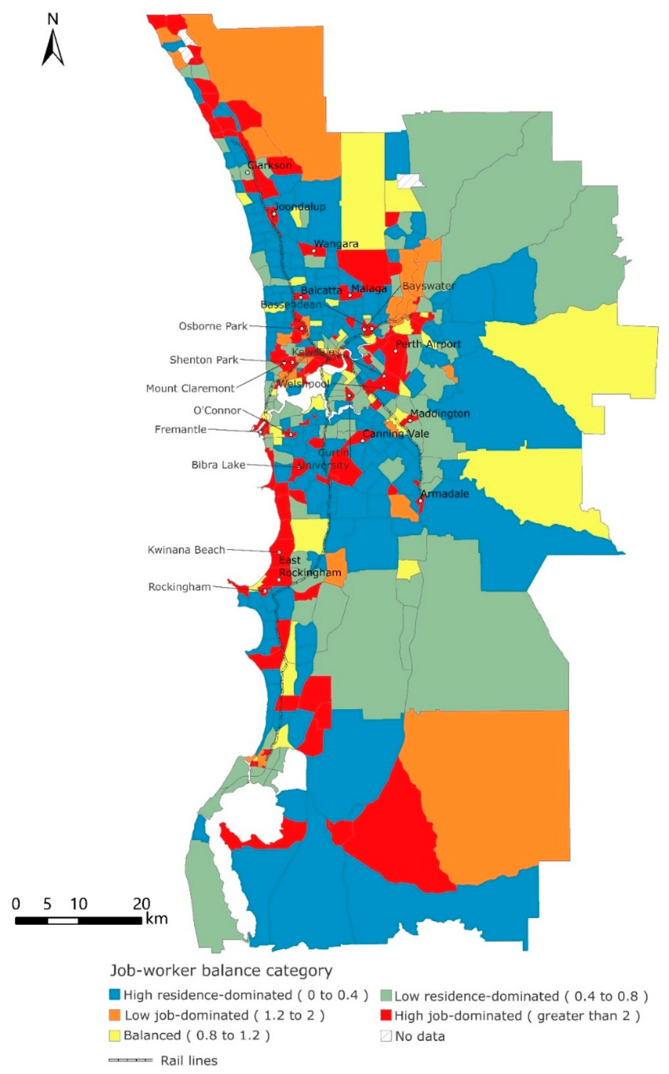
Figure 2 shows the spatial distribution of JWB in the PMR. Since many zones fall outside of the balanced range, we have further divided ‘residence-dominated’ and ‘job-dominated’ categories into two sub-categories each. Thus, zones with JWB ratios in the range 0.8–1.2 are balanced, 0–0.4 is high residential dominance and 0.4–0.8 is low residential dominance while 1.2–2 is low job dominance and greater than 2 is high job dominance.

Out of the total of 472 zones in the PMR, 436 had sufficient data for JWB calculations. The majority of these zones are in the categories of 0–0.4 (40% of zones and 15.3% of trips) and >2 (25% of zones and 61.1% of trips). According to our classification, these zones are either highly residence-dominated or highly job-dominated with a very small portion of mixed land use. Only 9% of the zones (6.3% of trips) are in the balanced range. Further, we have checked the spatial distribution of JWB in accordance with the city’s broader land use pattern. Residential dominated areas are identified along transport corridors and rivers (Swan and Canning). The major job concentrations occur in the City of Perth (CBD), which provides 17% of the total employment [50]. Biermann and Martinus [51] ascertain that Perth CBD has “an excess of job opportunities in relation to the local resident labour force” (p. 390).

Zones around industrial concentrations (e.g., Welshpool, Kewdale and Kwinana) are evidently job-dominated with higher JWB values. A similar clustering of job-dominated zones occurs around the North-East and North-Western fringes (e.g., Joondalup, Wanneroo, and Swan areas), mainly “driven by the transport, manufacturing and construction industries, generating a rapid growth in the number of people commuting into this sub-region from other parts of Perth” [50] (p. 229). Biermann and Martinus [51] further explain that “agriculture, forestry and fishing, education and training, accommodation and food services and retail trade are the industries most linked to internal travel within the North West sub-region” (p. 392). City fringes along the North-West (Swan and Wanneroo) and South-East (Peel) show an unlikely job dominance, which is due to the existence of large tracts of agricultural land with very low population densities, i.e., zones with relatively low employment levels but much lower population levels. It is worth noting that a much poorer balance is particularly seen around the two comparatively newer north-south train lines (Joondalup line and Mandurah line). However, a few places along the older transport corridors have grown over time in response to the natural integration of land and transport, or have strategically done so through transit oriented development (TOD) projects.

4.1.2. Spatial Distribution of ESS and ESC

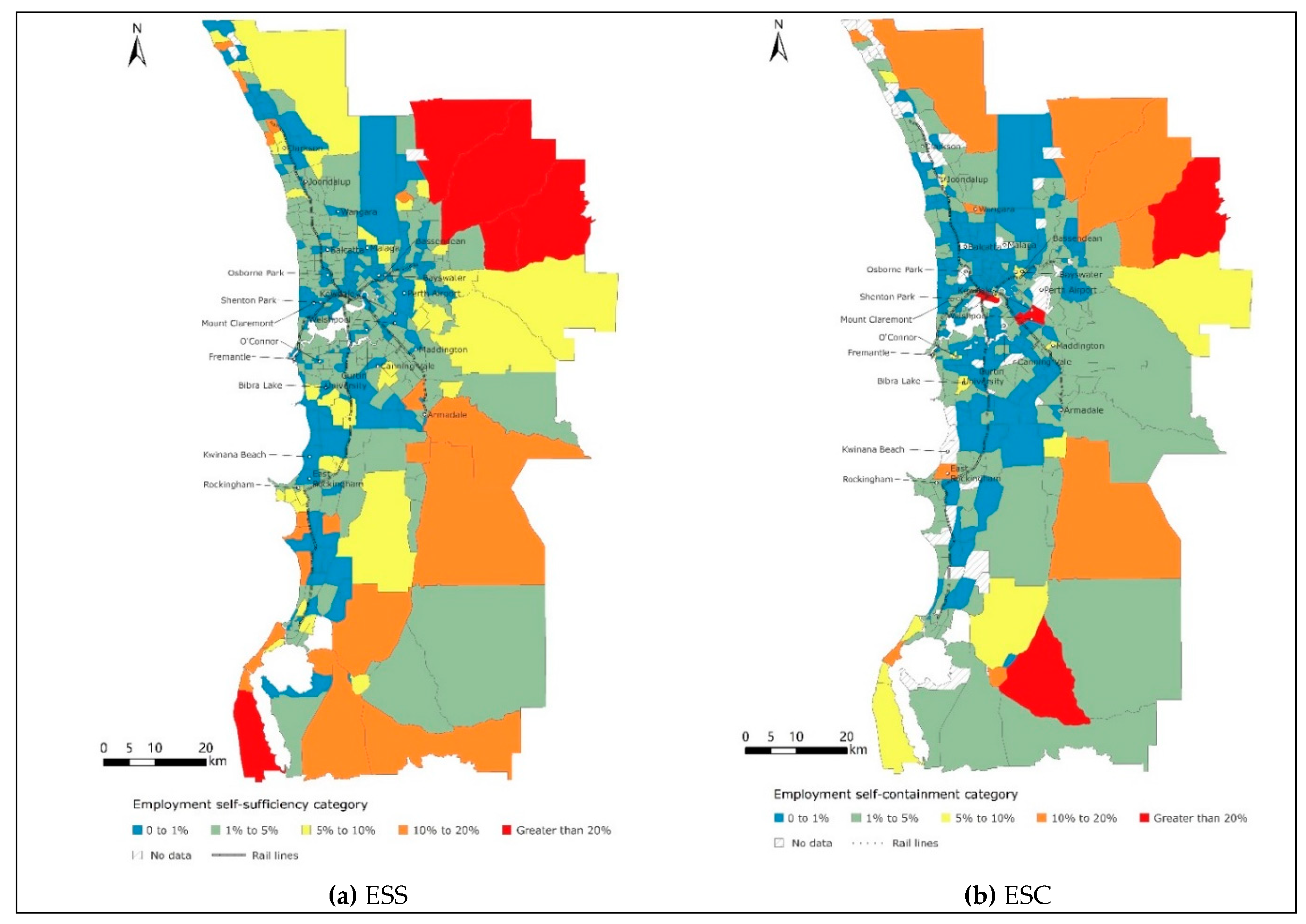
Generally, most areas in the PMR have very low ESS, meaning that there are not many jobs occupied by people living in the same zones (as their jobs) (see Figure 3a). Over 72.4% of zones, containing 71.1% of total workers, have ESS values less than 5%. Only five zones have a self-sufficiency level of more than 20% (containing only 1.3% workers) and they are all at the fringes.

The general spatial pattern of ESS shows a gradual increase from inner Perth to outer Perth. This means that a higher proportion of local jobs are filled by local resident workers in outer Perth as compared to the inner Perth where a lot of commuting is done into the area (Figure 3a). Agricultural areas close to the city edge are comparatively self-sufficient (ESS is >10%). In contrast, CBD, inner suburbs and more developed areas have appeared as less self-sufficient. It is evident that the CBD accommodates the highest number of jobs which are filled by workers coming from outside, leading to a high volume of inflow. It is noted that even some of the job-worker balanced zones have the poorest self-sufficiency (e.g., Balcatta). This indicates a potential mismatch between the type of local jobs and the occupation of the local resident workers.

For the ESC index (Figure 3b), we were able to examine 384 zones. About 81% of zones (containing 95% of workers) have ESC less than 5%. Only four zones have an ESC greater than 20%, and these are the CBD, Welshpool-Kewdale area and two other fringe zones. It is worth noting that the high values in fringe zones are due to low populations in these zones whereby a few agricultural workers make up a significant portion of the total resident workers.

As seen in Figure 3, the general pattern of spatial distribution of ESC is similar to that of ESS. This suggests that outer regions have fairly higher proportions of resident workers working locally, as compared to the inner parts of the city. However, there are slightly more zones with an ESC of less than 1% (46% of zones) compared to those with an ESS of less than 1% (42%). The very low ESC (<1%) zones are more concentrated in the inner regions, while the very low ESS (<1%) zones are mainly distributed around inner areas, i.e., along train lines, especially Fremantle and Midland lines, and North-West and South-West coastal areas. None of the zones have achieved a score even close to the target self-containment rate of 60% in the metropolitan area.

4.2. Spatial Pattern of Inflow and Outflow Travel Times

As already indicated, the effectiveness of the JWB, ESS and ESC indices is limited by the arbitrary nature of the geographic scale used. Also, these indices treat all external trips (long or short) the same, which can make the commuting situation look worse than it really is. Incorporating average commute times into (inflow), and out of (outflow), the zones can help to give a truer picture of the extent of commuting across the zone boundaries.

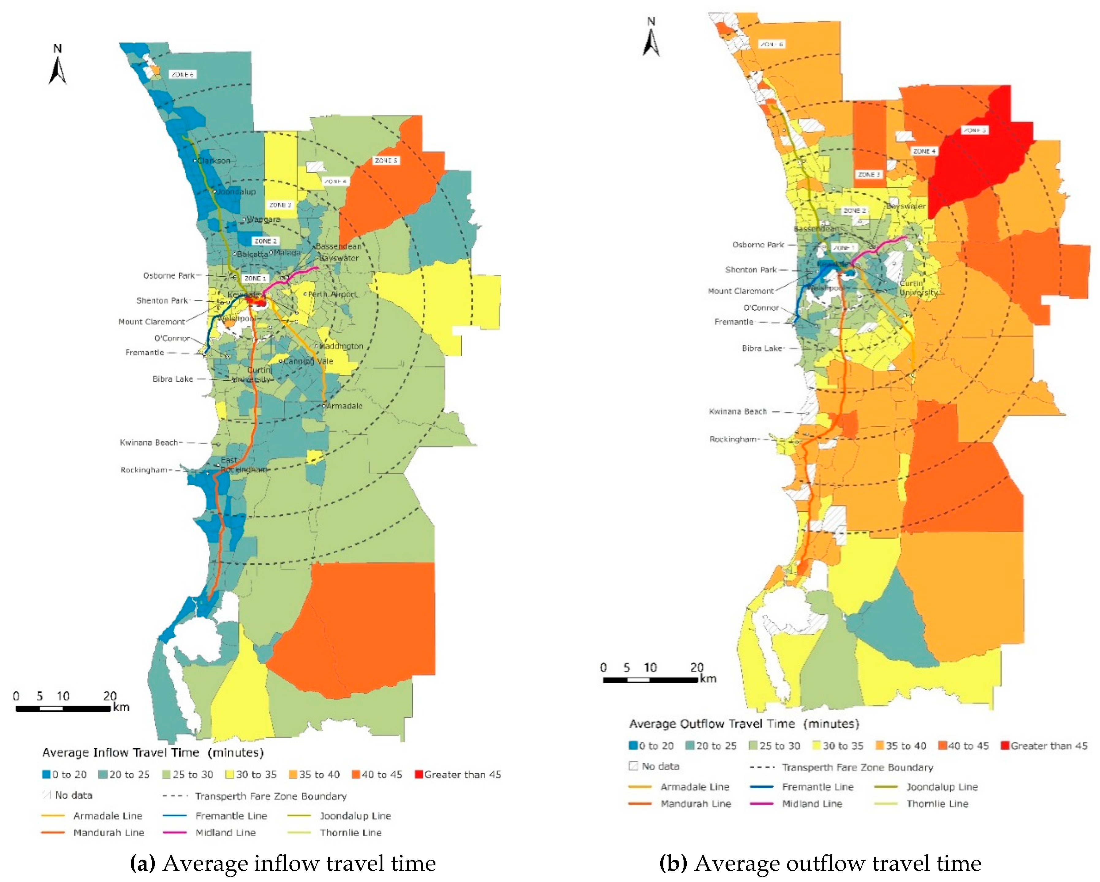
Inflow travel time is the average duration of trips from other zones coming into a target zone for work purposes. Figure 4a shows the spatial pattern of average inflow travel time in the PMR. The result uncovers a graduated decrease in average inflow travel time from the CBD to the Western edge along coastal lines, Swan River and train lines. Furthermore, an increasing trend in average inflow travel time was found towards outer Perth areas. Around 87% of the zones have an average inflow travel time less than 30 min, which is equivalent to Perth’s average commuting time [52].

The CBD has the highest average inflow travel time (>45 min) which can be attributed to the higher JWB ratio—the strategic nature of many of these jobs drawing from the region-wide labour pool–and Perth’s linear city structure. A few inner suburbs near the CBD (<20 km) with high job-dominance, have relatively higher average inflow travel times (30–35 min). These include Welshpool-Kewdale (industrial concentration), Curtin University (the second largest job destination region) and Cannington (one of the largest and most popular shopping centres in Perth). On the other hand, the commute times into most of the zones along the two newest train lines (Joondalup (opened in 1992) and Mandurah (opened in 2007)) and coastal areas (Western edge) are less than 25 min. While this may seem to suggest the contribution of train services in reducing inflow travel time, a more plausible explanation is that these areas have fairly non-skilled jobs which are filled more locally. The inflow travel time into zones along the older train lines, particularly the Fremantle line, is relatively higher (ranging from 25 to 40 min). On the contrary, these areas have more strategic/specialist jobs, e.g., hospitals, private schools and professional practices—which draw their workforce from a wider area.

Figure 4b shows the spatial pattern of average outflow travel time within the metro region. Outflow travel time is the average duration of all trips leaving a zone for work purposes. Apart from the CBD area in particular, most zones have higher outflow travel times than inflow times. Around 50% of the zones have an average outflow travel time less than 30 min. The outflow travel times show a pronounced concentric pattern: the lowest outflow time was in the areas around the CBD, which increased radially outwards. No obvious spatial patterns of the average outflow travel time around train lines are revealed. However, a noticeable distance impact of the average outflow travel time can be observed, which broadly coincides with the fare zones used by Transperth who run the various public transport modes within the PMR.

4.3. Relationships between the Employment Performance Indices and Travel Time

We summarised the average inflow and outflow travel times for each category of JWB, ESS and ESC (see

Table 1. Relationships between average travel time with respect to employment performance indices within the Perth metro region.

JWB (No. of Zones)			ESS (No. of Zones)			ESC (No. of Zones)
Inflow Travel Time (in Minutes)
	Mean	Std.		Mean	Std.
0–0.4(177 1)	23.62	3.74	>20% (5)	28.27	8.26
0.4–0.8(85)	25.58	4.53	10–20% (21)	22.13	4.33
0.8–1.2(39)	26.28	4.31	5–10% (40)	22.96	3.99
1.2–2(27)	26.54	5.71	1–5% (186)	24.94	4.71
>2(57)	26.27	5.73	0–1% (132)	25.93	4.67
Correlation	0.09		Correlation	−0.13
Outflow Travel Time (in Minutes)
	Mean	Std.					Mean	Std.
0–0.4	30.97	4.93				>20% (4)	25.83	9.12
0.4–0.8	31.06	6.02				10–20% (10)	37.09	8.27
0.8–1.2	29.18	6.12				5–10% (14)	30.78	5.76
1.2–2	28.82	7.6				1–5% (155)	31.59	5.68
>2	26.77	5.54				0–1% (255)	28.52	5.09
Correlation	0.12					Correlation	0.08

¹ Notes: There are 177 zones with the JWB value between 0 and 0.4. 55 zones had insufficient data and were not included in the study.

) to find their effects on commuting time. For JWB, 177 zones (about 36%) scored between 0 and 0.4. This reflects few job opportunities available in these zones, relative to the high number of residents. Only 39 zones (8.9%) have a balanced job-worker ratio. In terms of the relationship, we found that on average, as JWB increases, average inflow travel time also increases. This means that resident-dominated zones (zones with JWB less than 0.8) have shorter average inflow travel times than zones with JWB larger than 1.2, or job-dominated zones. The balanced zones are roughly in the middle in terms of inflow travel time, and not the shortest as would have been expected. Meanwhile, average outflow travel time displays a contra pattern, i.e., as JWB increases, average outflow travel time decreases. Thus, resident-dominated zones have longer outflow travel times than job-dominated zones. The average outflow travel times of balanced zones is in the middle. Nonetheless, the JWB correlations with both inflow and outflow travel times are quite low at 0.09 and 0.12 respectively (Table 1).

Table 1 indicates that 318 zones (about 73%) have a low ESS level of less than 5%. Only five zones had ESS above 20%, and interestingly, their average inflow travel times were found to be the highest (28.27 min). Nonetheless, the standard deviations of travel times for these zones were also highest. For the rest of the zones, there is a clear trend that as ESS increases, average inflow travel time decreases (as expected). The correlation is −0.13. Note that ESS only relates to inflow travel while ESC relates to outflow travel.

For ESC, about 81% of the zones were at less than 5%. For those zones with the highest ESC of above 20%, average outflow travel time was found to be the lowest at 25.83 min. However, there are only four zones in this category and the standard deviations are also highest. When considering all the zones, there was no obvious relationship between ESC and average travel time.

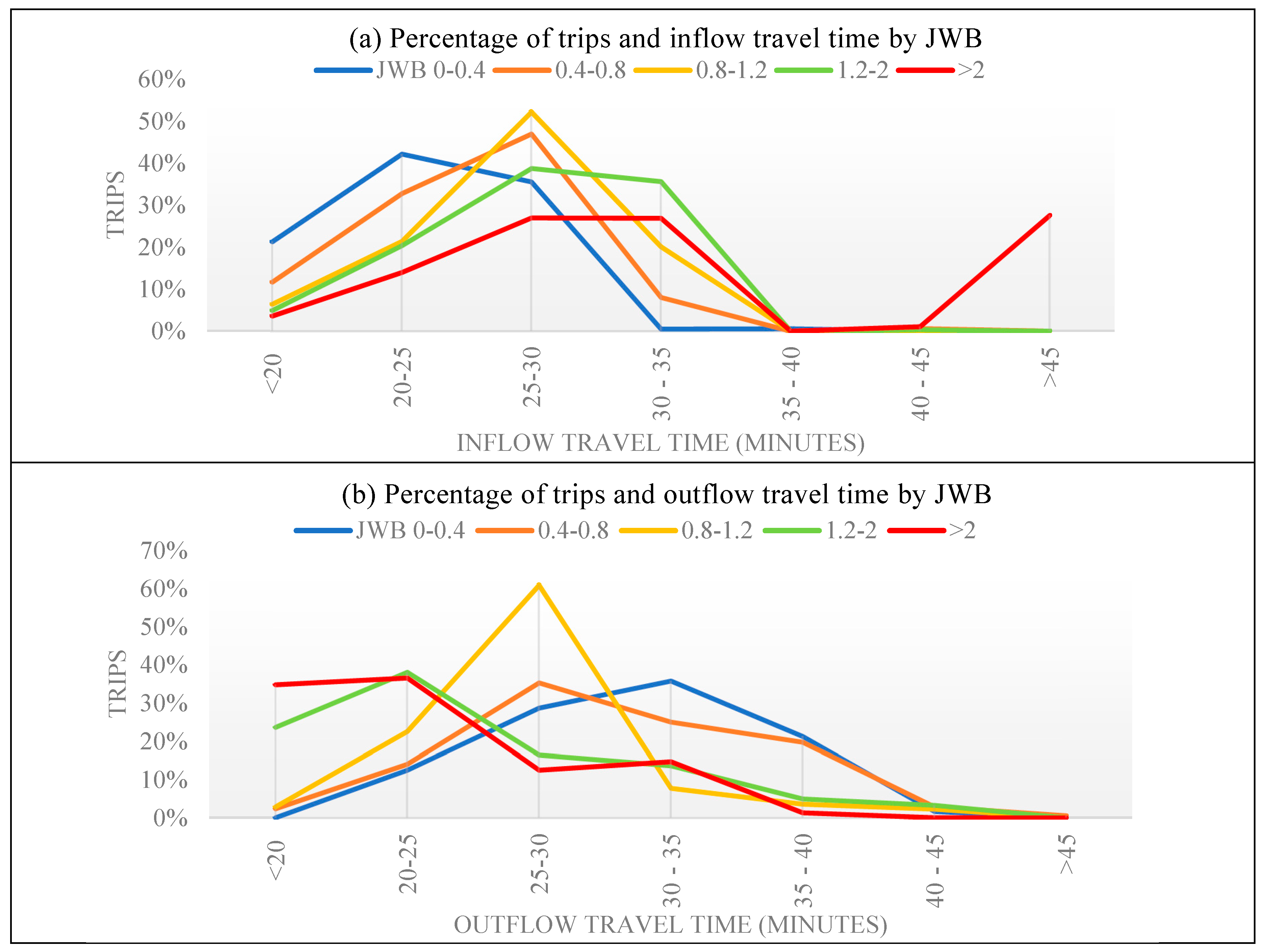
We have further assessed the relationships by taking the percentage of trips into consideration. A cross graphical plotting of trips, average travel time and employment performance indices shows the contra distribution of travel time (inflow and outflow) and JWB ratio. The graphs for lower JWB values, i.e., 0–0.4 and 0.4–0.8, are skewed towards shorter inflow travel times (see Figure 5a), while for outflow travel time, lower JWB values correspond with a longer outflow travel time (see Figure 5b). Conversely, the graphs for higher JWB, i.e., 1.2–2 and > 2, skewed slightly to the right, that is to longer inflow travel times (Figure 5a) while in the outflow travel time graph (Figure 5b), they are skewed to the left, or to shorter outflow travel time. For balanced zones (JWB: 0.8–1.2), the majority of trips fell in the 25–30-min bracket—over 50% for inflow trips and over 60% for outflow trips—with a more symmetric distribution compared to other zones.

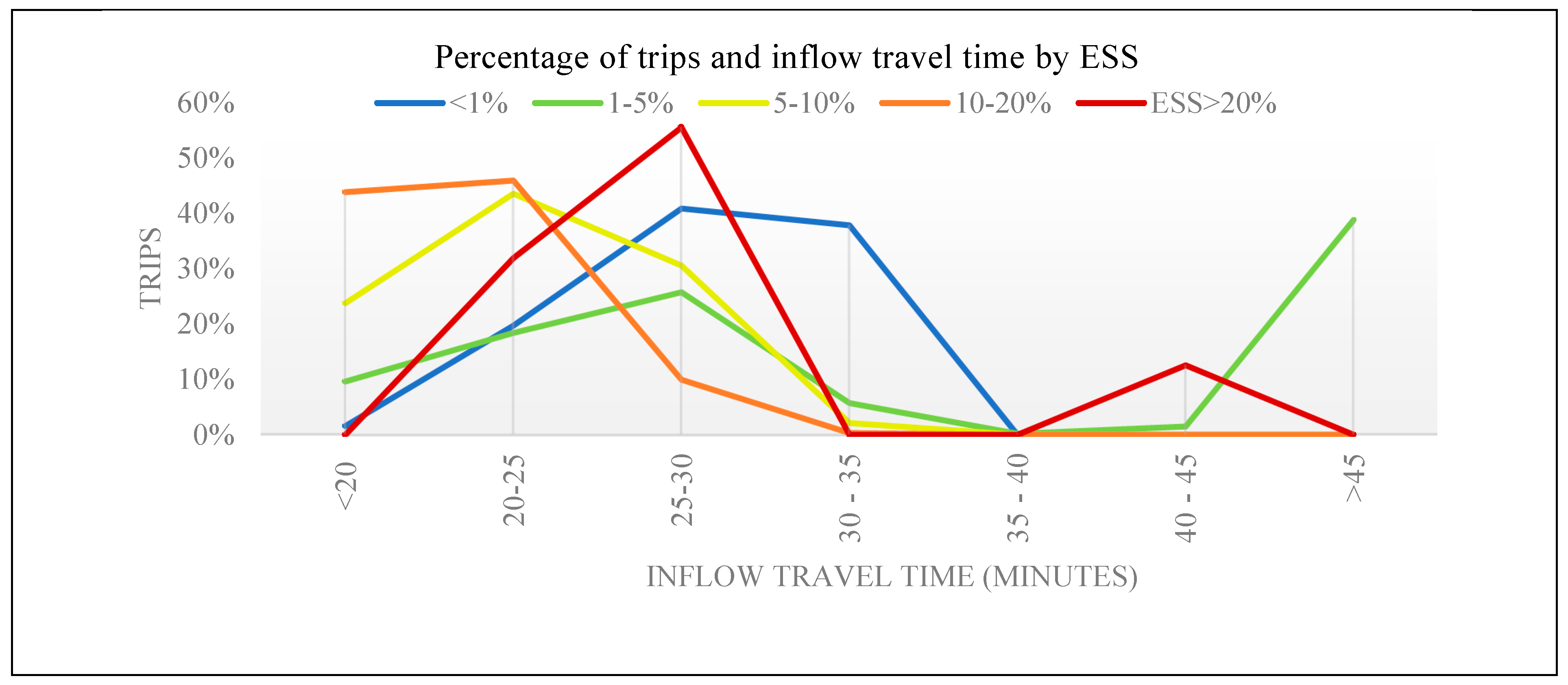
A similar three-dimensional comparison of ESS, trips and travel time (Figure 6) illustrates that in zones with ESS lower than 1%, 40% of trips have inflow travel time in the range of 25–30 min. For zones with ESS between 1% and 5%, over 40% of trips have inflow travel times longer than 45 min. In the case of higher ESS, the inflow travel time becomes shorter, with over 80% of trips taking 30 min or less (55% in the 25–30 min bracket and 32% in 20–25 min).

Based on the mean values of travel time at Table 1, it was difficult to identify a pattern between travel time and ESC. In the three-dimensional graph of trips and travel time by ESC (see Figure 7), the general trend in the relationship between ESC and outflow travel time is still difficult to discern. In zones with ESC < 1%, the percentage of outflow trips peaked at 25–30 min of travel time. While the highest proportion of trips from zones with high ESC (>20%) had the shortest average travel time, the other ESC categories’ graphs skewed to the longer travel times.

4.4. Spatial Interpretation of Relationships between Travel Time and Employment Performance Indices

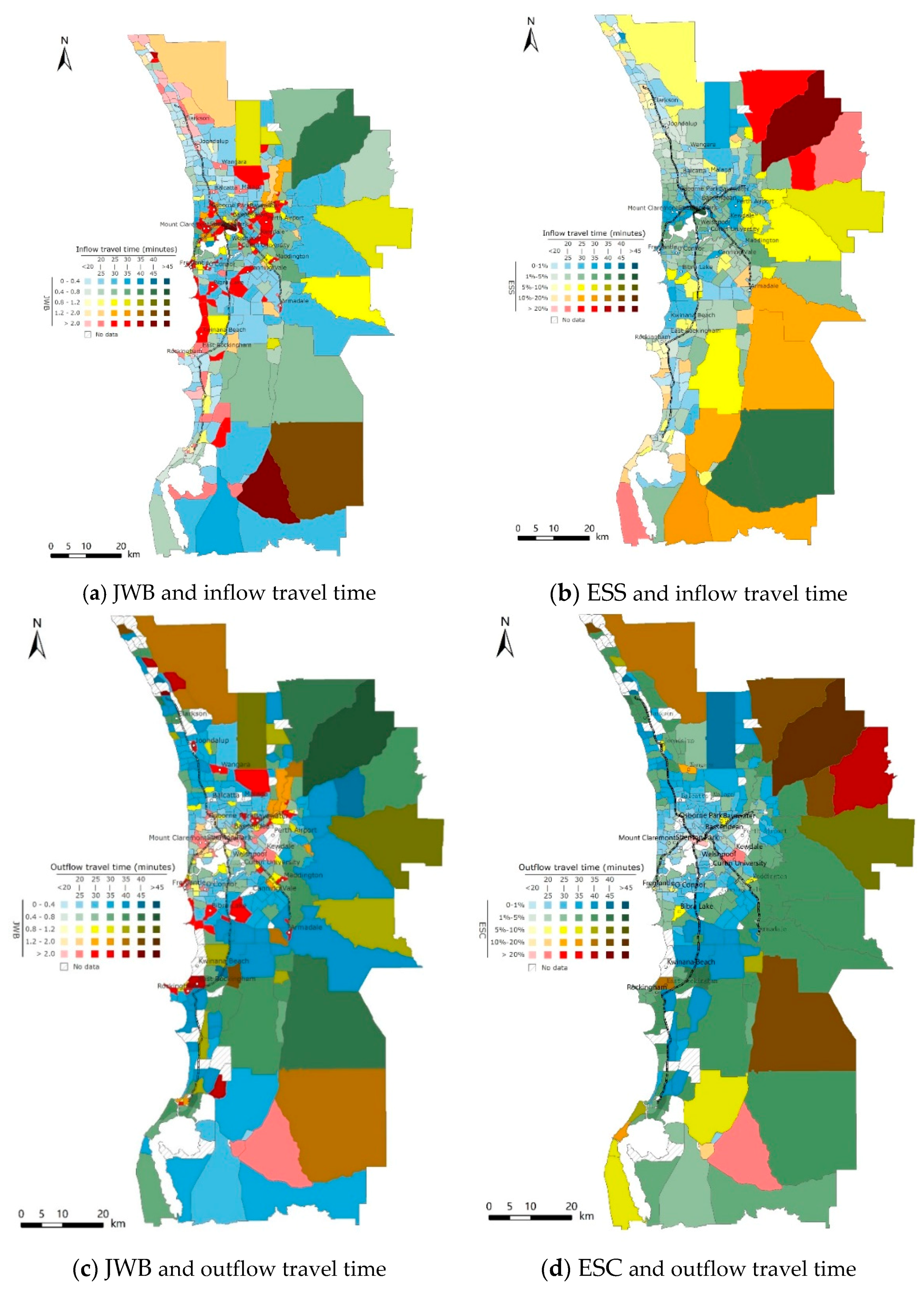
To determine the spatial dimension of travel time in relation to the employment indices, Figure 8a,b compare JWB and ESS in relation to inflow travel time. The interaction between spatial distributions of inflow travel time and JWB reveals that most zones located in the far Northern and Southern coastal areas have quite high JWB (some zones are at >2—job-dominated) and relatively low inflow travel time (under 20 min) (see Figure 8a). Most of these zones also have very low ESS (<1%) (see Figure 8b). We also observe across the two figures (Figure 8a,b) that where JWB is very high (>2), ESS is very low (0–1%). These areas have inflow travel times of less than 35 min. The relatively low inflow travel time in these areas indicate that while the proportions of jobs filled locally may be generally low, many of these jobs are filled by workers residing in the surrounding zones close by.

For zones located closer to the central areas, such as the CBD and areas around the Swan River, the inflow travel time is relatively high (>30 min). There is a mixture of zones with high JWB (some have >2; highly job-dominated) and low JWB in this area, while the ESS is very low (0–5%) for almost all of them. As identified in Section 4.2, the CBD has the highest average inflow travel time (47.5 min). It also has a very high value of JWB (23) and a very low value of ESS (1.4%). This means a ratio of 23 jobs available to one resident worker and approximately 98% of local jobs in the CBD are filled by non-resident workers. It is a heavily job-dominated zone with a wider worker catchment area, reflecting the monocentric spatial structure of job distribution in Perth.

The average inflow travel time to areas around the Fremantle line is also relatively high, mostly between 30 and 35 min. ESS is consistently low in this area (less than 1%). However, mixed values of high and low JWB appear in the area. This means some areas are job-dominated, while others are resident-dominated. These zones represent some of the oldest and opulent suburbs in Perth with many grand residential structures. There is also a concentration of major health and academic facilities such as Sir Charles Gairdner hospital and Queen Elizabeth II Medical Centre, University of Western Australia (UWA) and a number of renowned private schools.

The riparian zones between the Swan River (north) and ocean, and Welshpool/Kewdale regions notably have inflow travel times ranging between 30 and 35 min. These areas also have very poor self-sufficiency (ESS = 0–5%). Interestingly, none of the five most self-sufficient zones have inflow travel times in the lowest bracket of less than 20 min. Nevertheless, they—apart from one—do fall within the 30 min bracket. The size of these zones (outer zones are generally larger) could be the reason why they, despite having relatively higher ESS, do not have the lowest travel times in the region.

The job-worker balanced zones are distributed sparsely over the areas between job-dominated zones and resident-dominated zones. Their inflow travel times range between 25 and 30 min. The majority of these zones have relatively low ESS (0–5%), except for one, which is located at the edge of the PMR with an extensive boundary.

Figure 8c,d compares JWB and ESC against average outflow travel time. The majority of balanced areas (63%) are located along train lines and within 30 min outflow travel time. Unbalanced areas have a range of outflow travel times. Figure 8d demonstrates that higher ESC (>20%) have an average outflow travel times of less than 25 min. These zones include the CBD, major industrial areas and two outer Perth suburbs (Pinjarra and Chidlow). The lowest ESC is found in zones around the inner core (excluding the CBD zone), and these zones are evidently characterized by low outflow travel times. Self-containment data shows that the majority of resident workers in the PMR have to travel out of their local zones to work but their travel time becomes less if they live closer to the CBD. Nevertheless, all other zones in the outer suburbs have both low ESC and relatively longer outflow travel times (30 min or more), which is consistent with expectations.

5. Discussion

This study has examined the degree and spatial patterns of JWB, ESS, ESC and inflow/outflow travel times using household travel data in the PMR, and has empirically examined the interactions between these three indices and inflow and outflow travel times across the region. The findings reveal that the PMR has a poor JWB, with under 10% of zones being balanced. We further find out that these balanced areas do not necessarily have shorter commuting times. Resident-dominated zones had relatively shorter inflow travel times, but longer outflow travel times, while job-dominated zones had relatively longer inflow travel times and shorter outflow travel times. The travel times– both inflow and outflow–for the balanced zones were moderate. The results also demonstrate, and support the assertion, that higher ESS is associated with shorter inflow travel time. This is evident, for example, in the zones located in the far northern and southern coastal areas of the city, where the average inflow travel times were relatively shorter (<25 min) and the ESS was relatively high (ranging from 5% going to >20%). This suggests that local jobs may be filled by workers living within the zones or at least in the surrounding zones, thus keeping the travel times relatively low. On the other hand, the outflow travel times of these zones were relatively longer, at over 30–40 min. This can be expected given the low ESC in these areas. These areas accommodate some strategic metropolitan centres which are planned to generate significant employment opportunities and hence attract further attention to rethink on accessibility and inter-zonal networks. It is however, noted that the distribution of outflow travel time across the study area was not consistent with that of ESC, leading us to conclude that there is no clear relationship between the two.

The spatial pattern of outflow travel time was increasing radially from the central core, showing a resemblance to the city’s centralized public transport zoning system (see Figure 4b). This reflects the monocentric urban structure of Perth where commuting is characterized by a “strong radial travel to CBD and high public transport use to central locations” [54] (p. 47). However, the spatial pattern of inflow travel time indicates cold spots (areas with shorter travel time) around local and regional activity centres (e.g., Joondalup and Rockingham). This may show the effectiveness of decentralisation of jobs in reducing travel time.

The results have also shown that most of the zones are in the JWB category of 0–0.4 (40% of zones representing about 15% of trips) and >2 (25% of the zones representing 61% of trips). These zones are either highly residence-dominated or highly job-dominated with a very small portion of mixed land uses within the zones. Over 72% of zones containing 71% of workers, have an ESS value of less than 5%. On the other hand, around 81% of zones containing about 96% workers, have an ESC of less than 5%. This indicates that a large number of people are living and working in different zones in the PMR. This could be ascribed to the increasing trend of suburbanisation and decentralized job locations leading to higher commuting flows across the regions [52]. It suggests a spatial mismatch between jobs and residential locations as well as inter-regional disparity in terms of employment opportunities and housing provision [48,55]. Although job decentralisation is a priority in Perth’s urban planning and development agenda [15], it is proving difficult to relocate jobs from the central areas or move people into the job-dominated areas.

The findings of this study contribute to the growing debate on the effectiveness of JWB in tackling urban transportation problems and the distribution of economic resources. A number of studies have suggested that a decentralisation of jobs that is accompanied by balancing the number of local jobs and worker residences may lead to shorter commuting [23,34,35]. In effect, it may reduce general vehicle-miles travelled [56] and increase job opportunities close to the residents. Such strategies are inclined to take that opportunity to minimize disutility in city’s resource distribution policies [33]. While others argue that living close to work may not be a priority for many people, a complex range of other factors may influence residential location choices, such as housing affordability, quality of neighbourhood and quality of schools [27,52,57]. Therefore, policies solely relying on balancing the number of jobs and workers in certain areas may not be effective in reducing commuting time.

The study has produced the three standard indices, JWB, ESS and ESC, for the PMR, as well as additional indices based on average travel times to work into each zone as well as from each zone. The production and assessment of these indices have raised a number of methodological issues. The first was discussed earlier in the paper pertaining to the geographical scale chosen and associated MAUP. Dividing the study area into a few large zones would be likely to give better JWB, and potentially higher ESS and ESC levels than the results for the same area divided into many smaller zones, even though the underlying spatial distribution of jobs and workers remains the same. In addition, in the case of Perth (and likely in many other cities), zones tend to be selected based on the land use type and can be quite homogeneous. For example, a residential area would be one zone and an adjacent employment area a separate zone. This can result in poor JWB, ESS and ESC values for both zones. A different zone system that had, say, half the residential area and half the employment area in the same zone would give a different, and indeed better result.

ESS and ESC are essentially ratios of the work trips made within a zone to those entering or leaving that zone. In addition to being susceptible to the MAUP, they also provide no information on, and take no account of, the length of trip made outside the zone. They only count trips crossing the zone boundary, not where these trips are going to or coming from, e.g., whether 100 m or 100 km away. Figure 5, Figure 6 and Figure 7 somewhat illustrate this problem, showing that zones within a given ESS or ESC band can have a wide range of average travel times. Hence, ESS and ESC provide no information on the external component of the trip. The JWB, ESS and ESC values derived for an area are very much a function of the zone system selected and therefore do not necessarily provide a reliable measurement of the efficiency of the work commute or the spatial balance between workers and jobs. The ability to reliably compare across a city, and indeed between cities, is therefore compromised. Additionally, containing trips is a difficult and complex task that both depends on and may lead to changes in the socio-economic make-up (e.g., wage levels) of the sub-regions due to the variety in commuting patterns of workers in different industries and occupations [12].

This paper presents two additional indices, the average travel times to work into and out of the zones (inflow and outflow travel times). As these simply use travel times between zones they are far less sensitive to the selected zone system and hence MAUP. Changing the zone system has little impact other than changing the zonal travel times (measured as zone centroid to zone centroid). In this case, reducing the zone size improves the accuracy of the results as travel times better represent all workers in a zone. Clearly, the indicators include time travelled outside the zone, removing the limitations of ESS and ESC. They also provide for more reliable and consistent measurement across a city and allow comparison between cities, largely independent and irrespective of the zone systems chosen.

Studies have previously identified some shortcomings of JWB and self-containment measures, where it was found that self-contained cities in Britain did not rely on sustainable modes of transport, but rather they were relatively auto-dependent. On the other hand, those towns that were less self-contained in France and Sweden had most of their external trips done by non-auto modes including rail [58]. Our findings further showed that the relationship between ESC and commuting time was an unexpected positive correlation, suggesting that self-containment does not lead to shorter travel times. While ESS and ESC measures might require more appropriately selected zones to allow for a good land use mix, there will always be some trips crossing the boundaries which are not fully accounted for. The above evidence suggests that policies aimed at directly cutting down commuting times for a majority of the commuters such as investment in fast rail transit and coordinated transit services may be more effective in reducing commuting times than self-containment initiatives. For cities with low density developments and low transit patronage such as Perth, densifying developments around transit stations has great potential to yield significant improvements by enabling more people to enjoy faster commutes by public transport.

The results of this study can provide critical insight to planners and policy makers in both large and growing cities pursuing commute reduction through JWB and trip containment objectives. City councils and governments relying on these measures should complement them with travel time (and/or other socio-economic factors) to increase their reliability and reflect a truer picture of the commuting situation.

6. Conclusions

This paper sought to evaluate the levels of JWB, ESS and ESC in the PMR, assess their spatial patterns and examine their impact on commuting time. Using STEM zones as the geographic scale, we found that the levels of all the three indices were rather poor/low across the region. The JWB analysis revealed that balanced zones were few and far between; only 9% were balanced. Most zones fell to the extremes; either highly residence-dominated (40% of zones) or highly job-dominated (25% of all zones). An overwhelming majority of zones are under 5% of both ESS and ESC, and only very few zones are above 20%.

For balanced zones, the majority of trips fell in the 25–30-min bracket—over 50% for inflow trips and over 60% for outflow trips. However, the shortest inflow travel times were in residence-dominated zones (and not balanced zones), while job-dominated zones had longer inflow times. The outflow travel times, on the other hand, were longer in resident-dominated zones and shorter in job-dominated zones. The general relationship between ESS and travel time showed that inflow travel time gets shorter with an increase in ESS. The relationship between ESC and travel time was inconclusive. Outflow travel times were lowest in the CBD, a stark opposite to outflow times. Also, most zones (apart from the CBD) had longer outflow than inflow travel times. Overall, the inflow travel times were not too high (most were under 35 min), considering the rather poor levels of JWB and ESS across the entire metropolitan region.

Findings of this study show that JWB, ESS and ESC measures do not give a complete picture of the level of commuting. Due to their failure to account for the external part of the trip, planning policies relying on these measures (1) could lead to a misdiagnosis of the commuting situation, and/or (2) may not lead to the desired commute reduction. The proposed additional travel time indices address the above issues and are considered to be more reliable indicators of the efficiency of the work commute. Thus, we recommend that planning policy that relies on these measures also incorporates a component that accounts for the part of trip that is outside the zone, such as travel time, to better represent the commuting situation. Future studies should explore these indices in more cities and a wider variability of land uses to refine these results and enable generalisation to a wider variety of contexts.