Article

Natural and Human-Induced Drivers of Groundwater Sustainability: A Case Study of the Mangyeong River Basin in Korea

1
Institute of Natural Sciences, Yonsei University, Seoul 03722, Korea
2
Groundwater Laboratory, Korea Institute of Geoscience and Mineral Resources (KIGAM), Daejeon 34132, Korea
3
Department of Earth System Sciences, Yonsei University, Seoul 03722, Korea
*
Author to whom correspondence should be addressed.
Sustainability 2019, 11(5), 1486; https://doi.org/10.3390/su11051486
Submission received: 7 February 2019 / Revised: 6 March 2019 / Accepted: 7 March 2019 / Published: 11 March 2019
(This article belongs to the Special Issue Sustainability of Water Resources in the Developing Cities)

Abstract

:
The sustainability of rural areas depends on the availability of water resources. The Mangyeong River Basin (MRB) in Korea faces a water supply shortage for agriculture and industry. Based on 11-year (2005–2015) precipitation and groundwater monitoring data, groundwater sustainability was evaluated in terms of natural and man-made factors and their spatio-temporal variations. A precipitation time-series revealed a declining trend, but there were different seasonal trends between wet and dry periods, with declining and rising trends, respectively. Groundwater hydrographs from five national groundwater monitoring wells showed temporal variations. Groundwater wells located in downstream areas showed both recharge from upgradient areas and local man-made impacts (e.g. from pumping), resulting in an ambiguous relationship between precipitation and water levels. However, other monitoring wells in the upstream areas displayed water level responses to precipitation events, with a declining trend. Using the standardized precipitation index at a time scale of 12 months (SPI-12) and the standardized groundwater level anomaly, meteorological and groundwater drought conditions were compared to infer the relationship between precipitation deficit and groundwater shortage in the aquifer. The SPI results indicated severely dry to extremely dry conditions during 2008–2009 and 2015. However, the standardized groundwater level anomaly showed various drought conditions for groundwater, which were dependent on the site-specific hydrogeological characteristics. Finally, groundwater sustainability was assessed using water budget modelling and water quality data. Presently, if groundwater is used above 39.2% of the recharge value in the MRB, groundwater drought conditions occur throughout the basin. Considering water quality issues, with nitrate being elevated above the natural background, this critical abstraction value becomes 28.4%. Consequently, in the MRB, sustainable groundwater management should embrace both natural and human-induced factors to regulate over-exploitation and prevent contamination.

1. Introduction

Global climate change is an ongoing phenomenon that affects atmospheric processes and the water cycle, including air temperature, evapotranspiration, and precipitation characteristics (e.g., amount, type, frequency, and intensity). Consequently, there may be changes in hydrologic conditions, including sea levels, water levels, rainfall patterns, and drought occurrences [1,2,3,4,5]. Changes in the water cycle ultimately affect ecosystems, including human societies (e.g., due to irrigation, groundwater pumping, and dam or bank construction), by altering the potential availability of water resources [6,7,8,9,10]. In addition, human-induced climate change can also impact on changes in the hydrology [11,12].
The deficiency of precipitation leads to a reduction in available water resources, and its impact is propagated through the hydrologic system at different time scales [13,14]. Meteorological drought due to low precipitation can cause insufficiency in soil moisture and available water for plant growth and farming activity (i.e., agricultural drought), and the reduced recharge may cause a water level decline in the aquifer, resulting in groundwater storage deficiency (i.e., groundwater drought). A decline in the groundwater level subsequently causes a reduction of baseflow discharge to surface waters, resulting in stream depletion, land subsidence, seawater intrusion in coastal areas, and water quality degradation [15]. Thus, the effects of climate change on water resources, complicated by human induced factors, vary constantly in time and in space throughout the water cycle.
Groundwater, as part of the hydrological cycle, is an essential source of water for human use, such as in agricultural, industrial, and domestic activities. It generally flows through the porous medium at a very slow and steady rate. These semi-linear characteristics make it possible to predict changes in groundwater storage and, eventually, the related water resources, including surface water and groundwater-fed reservoirs. Thus, the groundwater level can be used as an indicator of the available water resources in an unconfined aquifer in the watershed. Subsequently, temporal and spatial trends in precipitation and water level changes can provide important information about groundwater in aquifers, which can in turn facilitate the development of an effective management plan [16,17,18].
A water level decline due to a decrease in groundwater recharge can originate from reduced precipitation, natural discharge as baseflow, and/or the pumping of groundwater through overexploitation and unplanned development. When groundwater is depleted in an aquifer, recovery can take a long time because of the typically slow process of natural recharge. Therefore, to secure sustainable water resources, the trends and current status of both precipitation and recharge must be understood by evaluating long-term monitoring data.
In addition to the volume of water resources, water quality is another key factor for the sustainability of resources. Pollutants on the land surface of industrial and agricultural areas can be introduced into the groundwater through the recharge process and can eventually lead to groundwater contamination. Consequently, water of sufficient quality must be available as a resource for specific applications; thus, water quality monitoring is necessary for effective assessment of water resource sustainability. In terms of exposure to surface pollutants, the presence of confining layers could play an important role in determining the vulnerability of deep groundwater aquifers.
In Korea, more than 60% of annual precipitation occurs during the wet season (June to September), and the amount and pattern of precipitation has large spatio-temporal variability [19]. This variation, as well as abnormal climate conditions [20,21], creates problems for natural ecosystems and water resource management [22,23]. The Intergovernmental Panel on Climate Change (IPCC) has reported that global climate change could lead to increased flooding and drought, even in Korea [7], and these phenomena have in fact occurred in the last decade [24,25]. The duration and frequency of precipitation has decreased, while the intensity of heavy rainfall events has increased [23], resulting in negative effects on groundwater recharge. Rainfall exceeding the infiltration capacity of the soil results in much of the precipitation being flushed away as surface runoff rather than being available for groundwater recharge [26]. Consequently, groundwater storage becomes deficient and more pumping wells are subsequently established, resulting in a vicious cycle of water resource depletion. In agricultural and rural areas, where the piped water supply is relatively poor [27], the effects of climate change have the potential to cause natural disasters affecting residents [28]. In addition, the use of agricultural chemicals (e.g. pesticide and fertilizer) degrades groundwater quality [29,30].
The present study area, the Mangyeong River Basin (MRB), is located in Jeollabuk-do, in the southwestern part of Korea (Figure 1). The river basin is characterized by a variety of land-uses and includes urban areas, industrial complexes, forests, and agricultural areas that are largely located on the Honam Plain, one of the largest plains in Korea. Since 2000, meteorological and agricultural drought events have occurred frequently in the basin, threatening the sustainable development of communities in the area in terms of water resources, especially given that groundwater is the main water supply for industry and agriculture. Thus, the aim of this study was to identify whether such droughts, as a measure of water resource sustainability in the MRB, could be attributed to natural (e.g., climate change) and/or human-induced drivers (e.g., groundwater exploitation and contamination), and to assess spatial variation in groundwater sustainability with long-term changes in these drivers.

2. Materials and Methods
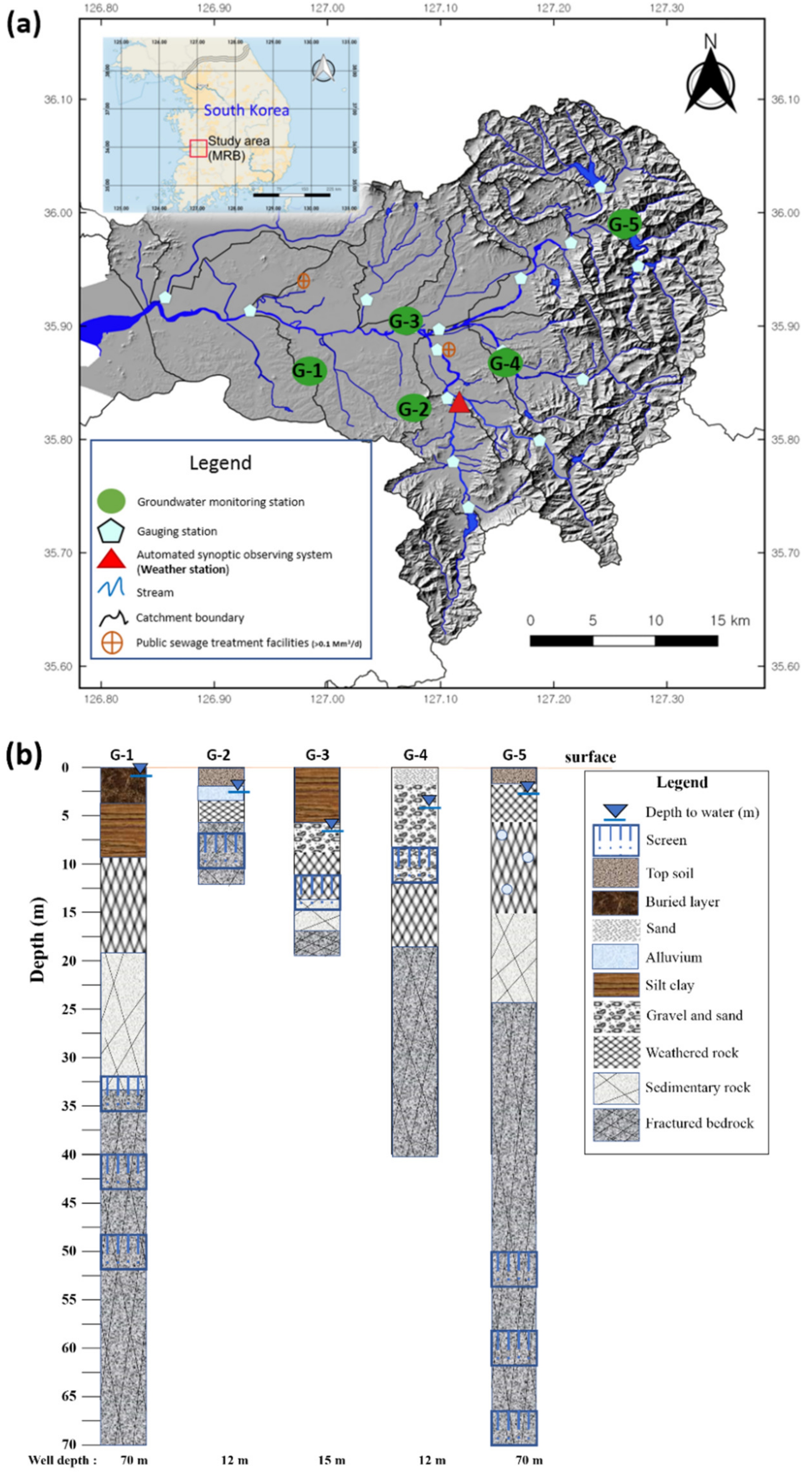
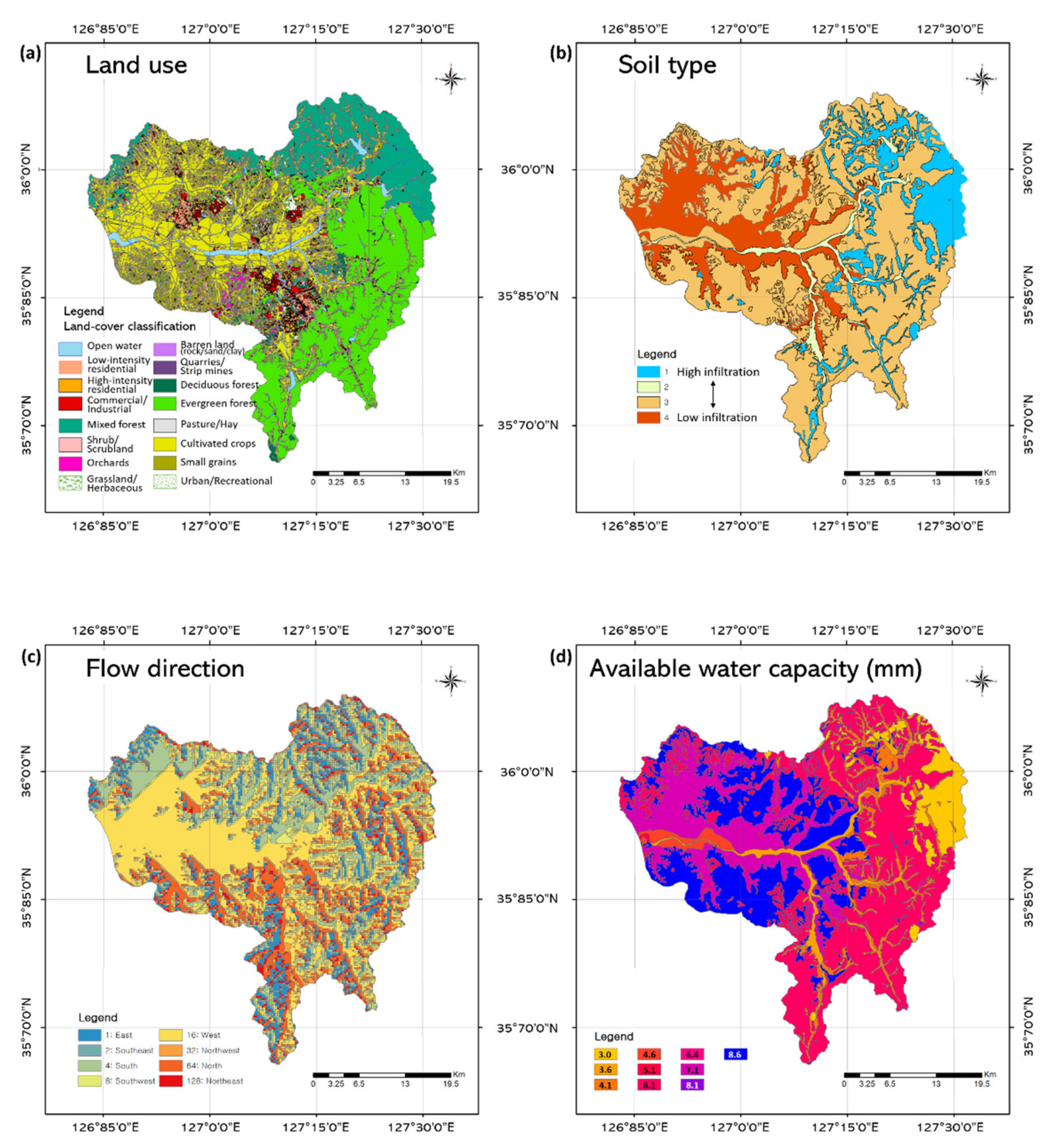
2.1. Study Area

The MRB is located in the southwestern part of the Korean Peninsula (between 35° 37’ to 36° 6’N and 126° 48’ to 127° 21’E; Figure 1a). The river basin covers an area of about 1,600 km2, with surface elevations ranging from 0 to 1,112 m (average: 124 m) and an average slope of 25%. The river basin is characterized by a variety of land-uses and includes urban areas, industrial complexes, forests, and agricultural areas. Mountain areas are distributed in the eastern part of the catchment, with plains (the great Honam Plain, which is one of the largest plains in Korea) in the west (Figure 2a). The river basin has a population of approximately 1 million. The end of the western part of the basin is adjacent to the coast and contains areas of reclaimed land. An estuary barrage was constructed in the downstream area to prevent flooding with seawater. The land use is approximately 42% farmland, 41% forest and 9% urban area, 5% water body, and others 3%, with a mean annual precipitation for 2005–2015 of about 1267 mm [32].
The study area is at the southwest end of the Okcheon Supergroup, which developed in the SW–NE direction across the Korean Peninsula and consists of metamorphosed sedimentary rocks of Precambrian to unknown age. There have been local intrusions and eruptions of Cretaceous acidic granitoids and Bulguksa granite. The alluvial layer of the late Quaternary is covered with an unconformity (MLTM [32] adapted from KIGAM, www.kigam.re.kr). The downstream part of the river bed is mainly composed of silt and clay, and the upstream part is composed of sand and gravel.

2.2. Data Acquisition

Both groundwater and rainfall monitoring data from the period 2005–2015 were analyzed to evaluate trends in rainfall and water level fluctuations. Groundwater monitoring data from five observation wells (G-1–G-5; Figure 1a) and climate data including precipitation, air temperature (minimum, maximum, and daily average), and evaporation in the MRB were obtained from the National Groundwater Monitoring Network (NGMN) of the Korea Water Resources Corporation (K-Water) and the Jeonju weather station operated by the Korea Meteorological Administration (KMA, http://data.kma.go.kr), respectively. The K-Water publishes an annual report of monitoring data, field surveys, and simple statistical analyses, providing general information about the area, and on the watershed, monitoring wells, and groundwater usage through the National Groundwater Information Center (GIMS). In this study, basic information about the catchment, and geological logs of the monitoring wells (Figure 1b), hydrogeological properties, water level data (Table 1), field survey and test results (permeability, specific yield and aquifer media), water quality characteristics, and groundwater use were obtained from GIMS (www.gims.go.kr) and the Ministry of Environment (ME, www.me.go.kr). Statistical analyses, such as trend and correlation analyses, were conducted using data provided by the Water Resources Management Information System (WAMIS, www.wamis.go.kr), including the total amount of annual groundwater abstraction and details of the public water supply system. Geographic information system (GIS) data on geological properties (catchment boundary, slope, elevation, stream line, soil group, and land use) were collected from WAMIS and the National Geographic Information Institute (NGII, www.ngii.go.kr) (Figure 2). However, while we aimed to use a complete dataset for 2005–2015, water quality data were available since 2008 and there were some missing values in the reports, causing some uncertainties and limitations in our interpretation.

2.3. Methods

2.3.1. Trend and Correlation Analyses

Linear regression (in this study, simple linear regression), a parametric method, is used to estimate the relationship between two variables and trends using the calculated slope of an equation [34]. The simple linear regression is written as the following Equation (1):
y = β 0 + β 1 x + ε
where, y is the dependent variable, β0 is y intercept, β1 is the gradient or the slope of the regression line, x is the independent variable, and ε is the random error.
However, the parametric method is affected by missing values or outliers of the raw data. In this study, to evaluate temporal trends in precipitation and groundwater levels, non-parametric statistics (Mann–Kendall test and Sen’s test) were used because, apart from not requiring normal distribution and homoscedasticity of the data, they offer the advantage of accommodating data gaps (missing measurements) and outliers in a time-series [35]. The Mann–Kendall (M–K) test, developed by Mann [36] and Kendall [37], computes the S statistic (S) as the time series of n data x (xi and xj; i > j), in the following equations:
S = j = 1 n 1 i = j + 1 n s i g n ( x i x j )
s i g n ( x i x j ) = { + 1           i f   x i x j > 0       0         i f   x i x j = 0 1         i f   x i x j < 0
where xi and xj are the data values at times i and j [38]. In addition, the standard normal variance (Z) can be obtained by assuming that the S statistic is normally distributed in cases where n > 10 [39]. Based on the significance level α, statistically significant positive (increasing trend; Z > 0) or negative (decreasing trend; Z < 0) changes were identified, and the data are considered to have no trend if Z is not bigger than the value corresponding to the 1–α/2 quantile value of the standard normal distribution.
Sen’s test is another non-parametric method to identify any trend of time series [40]. This test calculates a slope that determines Sen’s trend estimator. The median is obtained by listing the derived slope estimates in order of size, and the variance estimate for testing the hypothesis is obtained following the method of Kendall [37].
The water level change in the MRB was analyzed according to precipitation patterns based on monthly mean values during the 11 years from 2005 to 2015, and correlation coefficients were identified using the Spearman method. The Spearman’s test is a non-parametric rank-order test, and the correlation between precipitation and hydrological time-series using this method was reported by Kahya and Karayci [41]. The correlation coefficient (r), which expresses the degree of correlation between variables, has a value between –1 and +1. The closer the value is to –1 or +1, the stronger the negative or positive correlation, respectively. If there is no correlation between two variables (i.e., no trend), the correlation coefficient is 0 [37].

2.3.2. Spatial Variation of Groundwater

The spatial variation of groundwater in the study area was assessed in terms of both quantity and quality according to changes in groundwater recharge, and the amount of abstraction and distribution of nitrate in groundwater, respectively. Groundwater recharge can be evaluated by using water budget with seepage meters [42,43], tracers [44,45], modelling [46,47], and groundwater level change [48]. To analyze the water budget and estimate the groundwater recharge in the MRB area, we used the soil–water balance (SWB) model, which has been applied in various studies to understand the impact of future climate change and anthropogenic effects on groundwater resources [49,50,51]. The SWB model integrates GIS-gridded datasets (land-use classification, soil properties, flow direction, and available soil–water capacity) with observed climate data (precipitation, air temperature, and evaporation). Based on a modified Thornthwaite–Mather SWB approach [52], it estimates groundwater recharge at daily time steps for each grid cell using the following Equation (4):
Recharge = (Precipitation + Snowmelt + Inflow) – (Interception + Snowfall + Outflow + Evapotranspiration) − △Soil Moisture
Using Equation (4), groundwater recharge was calculated as the difference between the inflow from sources and the outflow to sinks of water and soil moisture. In this study, the model was simulated based on daily climate datasets (mean temperature, precipitation, relative humidity, maximum temperature, minimum temperature, wind speed, minimum relative humidity, and % sunshine) for the 11 years from January 2005 to December 2015, and on gridded data (ASCII file) that was reprocessed using ArcMap (ESRI, version 10.1; Figure 2). In terms of the relationship between supply and demand (i.e., the inflow to and discharge from the aquifer, respectively), groundwater recharge can be defined as the addition or entry into the saturated zone of water made available at the water–table surface [53]. Precipitation is the main source of groundwater recharge, and numerous methods have been developed to quantitatively evaluate groundwater recharge for determination of the sustainable yield. Changes in groundwater storage for the basin were attributed to input (recharge, subsurface flow in) minus output (baseflow, evapotranspiration, groundwater flow out) using the following equation (5) of Healy and Cook [48] (modified from Schicht and Walton [43]):
Δ S g w = R + Q o n g w Q b f E T g w Q o f f g w
where R is recharge, Δ S g w is change in subsurface storage, Q o n g w Q o f f g w is net subsurface flow (includes groundwater pumping), Q b f is baseflow, and E T g w is evapotranspiration.

2.3.3. Drought Index

Precipitation deficiency has been studied using indices of meteorological drought, such as the standardized precipitation index (SPI [54]), and the Palmer drought severity index (PDSI [55]). The SPI is the most commonly used index because of its simplicity, where it includes only long-term precipitation records (at least 30 years) gathered from monitoring stations as input data. The long-term record is fitted to a probability distribution and then transformed into a normal distribution [56]. Because of the variability in precipitation, the SPI was estimated for periods of 3, 6, 9, 12, and 24 months. Precipitation for 12 consecutive months was analysed to reflect long-term precipitation patterns. Because 12-month SPI data are usually compared with streamflow and groundwater levels [56], we also analysed drought severity over a 12-month period. Meteorological drought conditions, classified by McKee et al. [54] based on the SPI value, were categorised as near-normal (from −0.99 to 0.99), severely dry (from −1.50 to −1.99) or extremely dry (−2 and less).
Meteorological drought due to precipitation deficit could lead to a lack of groundwater recharge, causing a decline in the groundwater level and groundwater storage in the aquifer, and thus eventually to a groundwater drought. Thus, groundwater drought can be extrapolated from a time series of water level changes. In this study, groundwater drought events were identified from the standardized anomaly of groundwater levels, which was calculated by: (1) normalizing the hydrological variables, (2) standardizing the normalized distribution by removing the means of the transformed variable (i.e., long-term monthly means), and (3) dividing them by the transformed standard deviation (σ) [57]. When the standardized anomaly drops below –1, it indicates drought conditions.

3. Results and Discussion

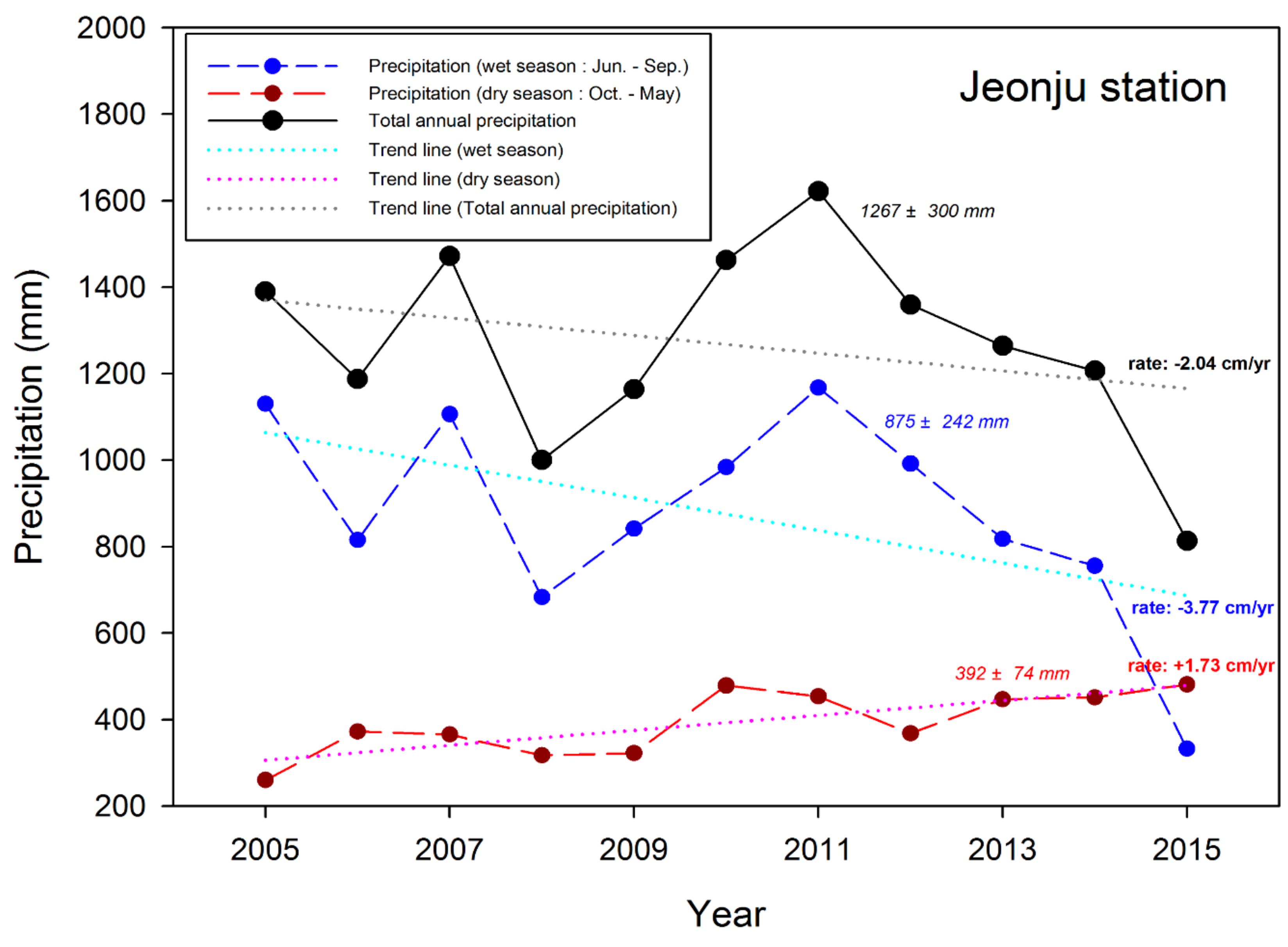
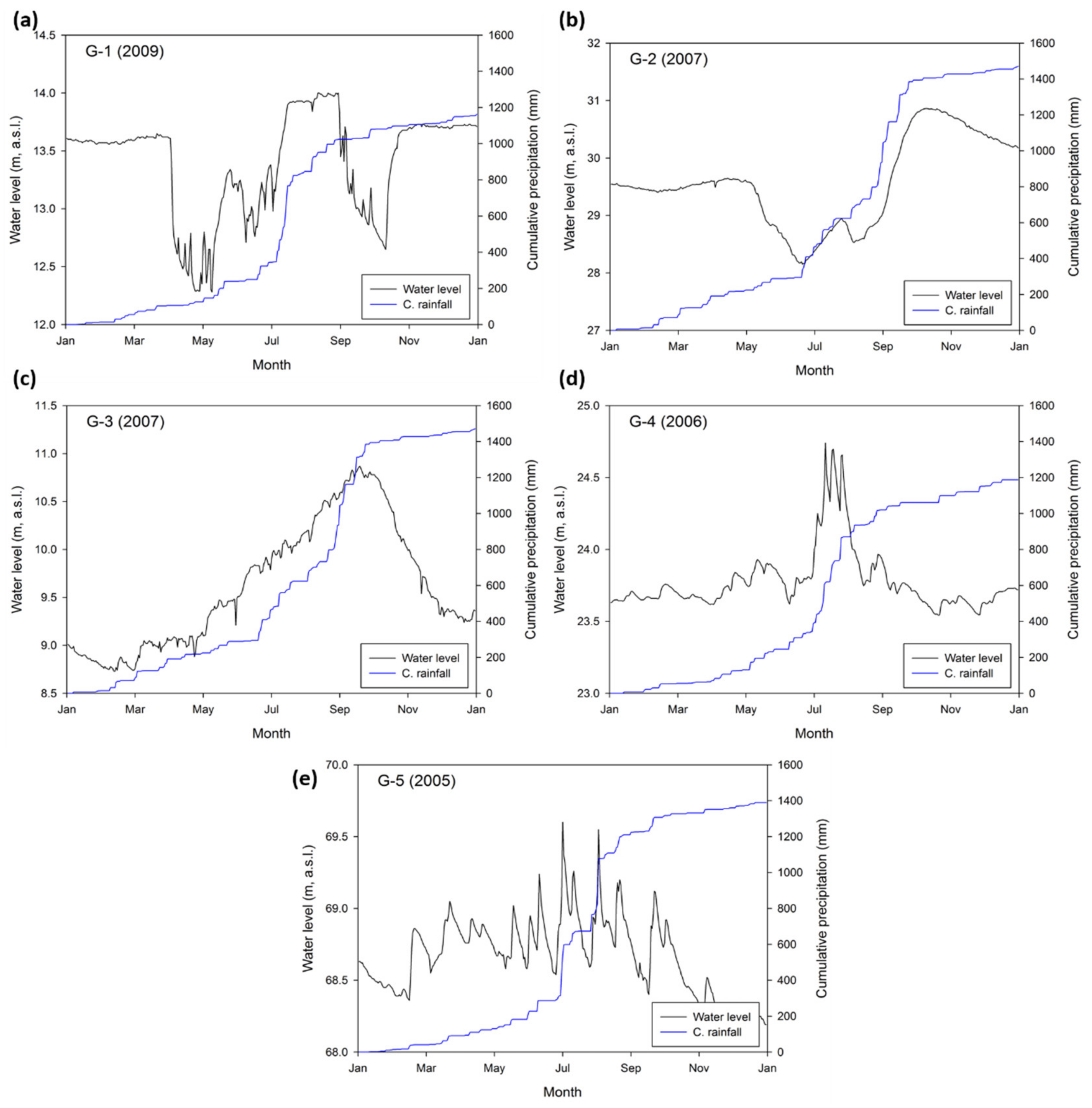
3.1. Temporal Changes in Precipitation

Because precipitation phenomena are subject to a large degree of temporal and spatial variation, it is difficult to identify fixed cycles or trends based on daily and monthly mean precipitation [58]. From 2005 to 2015, the total amount of annual precipitation displayed a declining trend of –2.04 cm yr−1, with significant yearly variations, and an annual mean (standard deviation) of 1,267 (± 300) mm (Figure 3, Table A1). Because Korea is under the influence of a monsoon climate, precipitation events can be distinguished in accordance with wet (June to September) and dry (October to May) seasons. In this study, the precipitation during the dry periods displayed an increasing trend, at a rate of +1.73 cm yr−1, while in wet periods there was a declining trend of –3.77 cm yr−1. Consequently, the trend in annual precipitation changes in the MRB area was influenced mostly by precipitation during the wet season. Because the amount of precipitation during the wet season accounted for the majority of the annual precipitation, a deficit of precipitation during this period could cause significant problems in the utilization of water resources. The difference in the amount of precipitation between the wet and dry seasons was smaller in years with drought events (366 mm in 2008 and 149 mm in 2015). In 2015, the amount of precipitation during the dry season was even larger than that during the wet season (Figure 3, Table A1). This significant change in the pattern of annual precipitation resulted in a “no trend” result in the non-parametric statistical analyses of the trend (Table 2).

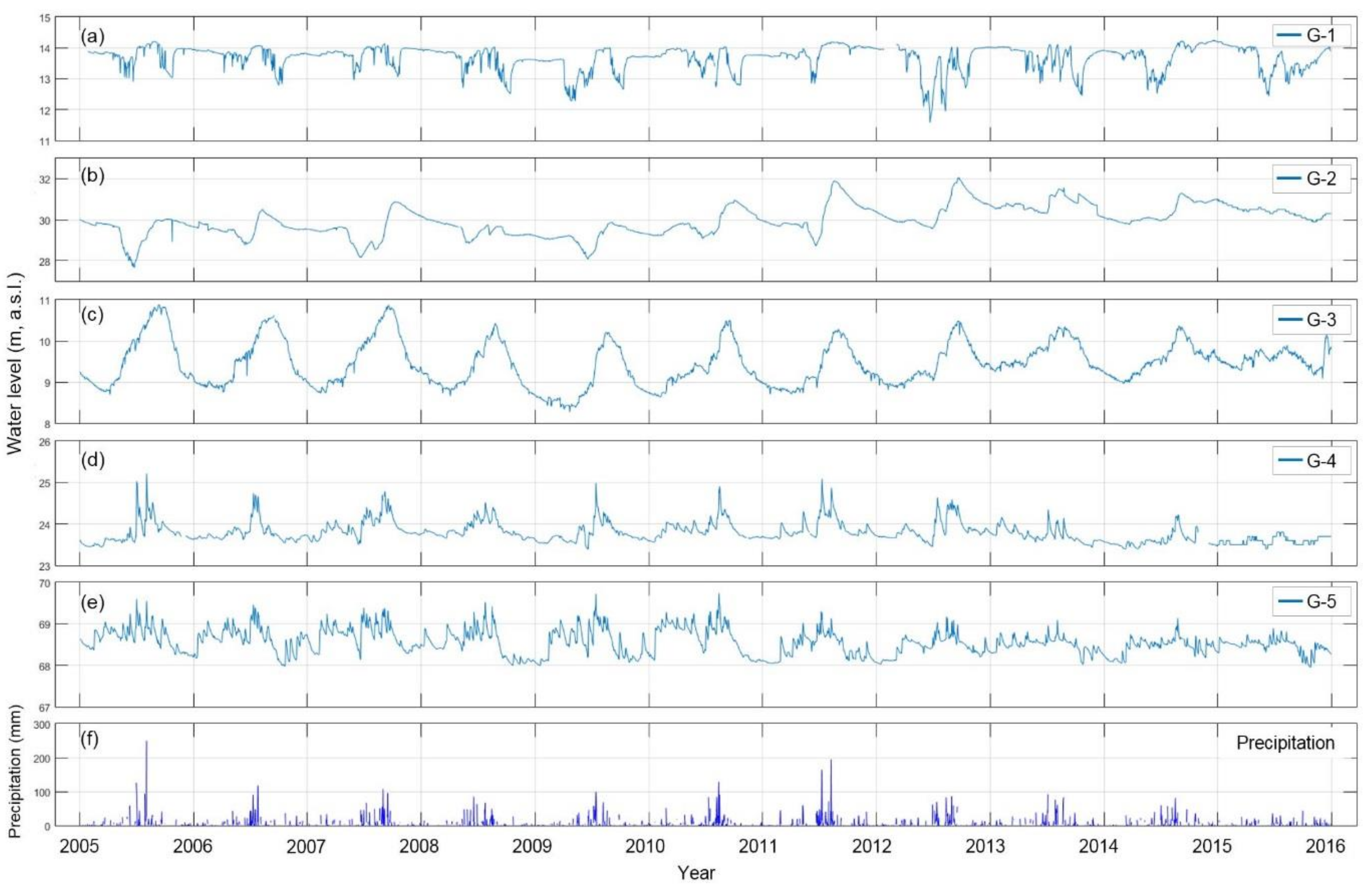
3.2. Spatio-Temporal Changes in Groundwater Levels

Groundwater hydrographs for the five monitoring wells in the MRB showed downward slopes at three stations (G-1, G-4, and G-5) and upward slopes at the other two stations (G-2 and G-3; Figure 4, Table 2). In the analysis of mean daily and monthly water levels, the M–K test results indicated an increasing (positive) trend at G-2 and G-3, and a decreasing (negative) trend at G-4 and G-5; at the remaining station (G-1), there was no trend at the 95% confidence level. According to Hirsch et al. [59], ‘no trend’ indicates that measurements over time are independent and identically distributed (i.e., not serially correlated). The results of the Sen’s tests were similar to those of the M–K tests, except for the monthly data at G-1.
The declining trend of both parametric and non-parametric methods for groundwater levels in wells G-4 and G-5 implied that they were relatively more influenced by precipitation during wet periods. In contrast, the groundwater levels in G-2 and G-3 displayed rising trends that reflected the influence of precipitation during the dry periods (Figure 3). Consequently, from the changes of water levels, wells G-4 and G-5 appeared to be in groundwater recharge areas, while G-2 and G-3 were in discharge areas where continuous groundwater inflows occurred. However, G1, located in a discharge area, showed no significant trends in non-parametric methods. Considering the depth of the well G-1, it could be attributed to the mixed signals of precipitation, pumping effects and lateral groundwater inflow from the upgradient recharge areas.
The water levels in two wells (G-1 and G-2) declined more sharply from May to June than during the post-monsoon period (September to May), while the water levels in the G-4 and G-5 wells exhibited steady declining trends. This pattern of water level decline in G-1 and G-2 indicated an additional driver of the water level decline, such as pumping for irrigation. Furthermore, even in the wet period, industrial activities placed a demand on groundwater resources (Figure 4).
The G-4 and G-5 wells were located in mountainous regions upstream of the basin. The rates of water level decline in the two wells were −1.83 and −2.56 cm yr−1, respectively. In 2005, 2007, and 2011, the total precipitation in the MRB during the wet season (1,130, 1,106, and 1,168 mm) was much higher than the average value for the other 10 years (846 mm, Table A1). However, the groundwater levels did not significantly rise in the periods (2005, 2007, and 2011), implying that rainfall with a high intensity could increase surface runoff, causing less groundwater recharge [51,60].

3.3. Spatial Variation of Water Level Changes

Spearman correlation analysis incorporating a lag-time, calculated according to the correlation between daily precipitation and water level data, revealed that the water levels of G-3, G-4 and G-5 were strongly correlated with precipitation, implying rapid rainfall recharge. However, G-3 had a trend towards a rising water level, which contrasted with the declining trend in G-4 and G-5. This difference was attributed to the locations of wells, with G-4 and G-5 being located in upstream recharge areas and G-3 being located in the downstream discharge area of the groundwater flow system (Table 1). In contrast, no significant correlation was found between the water level in G-1 and G-2, which were located in downstream lowland areas, and paddy field cover, where soil addition and irrigation pumping could complicate the water level responses to precipitation (Figure 1 and Figure 2).
The correlation between rainfall and groundwater water levels was also separately analyzed for the wet and dry seasons. The correlation coefficient for the relationship at G-1 was 0.366 for the rainy season and –0.162 for the dry season. Because the correlation differed seasonally, the increase in water level could be explained by groundwater recharge through precipitation percolation during the wet season. In the dry season, vertical recharge could be obstructed in the unsaturated layer, and human activities could influence the water level responses to rainfall events.
The correlation coefficient for the relationship at G-2 was –0.199 in the wet season and –0.233 in the dry season. Because the monitoring well taps into the alluvial unconfined aquifer, with a depth of 12 m (Table 2) in the rice paddy area, the weak correlation can be interpreted in terms of a greater effect of anthropogenic factors (e.g., pumping and irrigation), relative to natural factors, including rainfall and seasonal effects. Many mechanisms could lead to fluctuations in groundwater levels [53]. Especially in agricultural areas during the irrigation season, water level patterns show the mixing of precipitation recharge, pumping drawdown, and recovery after pumping. In the study area, Ha et al. [61] also reported the possibility of a weak correlation between precipitation and groundwater levels due to water abstraction or tidal effects related to the river stage.
The annual variation in precipitation and groundwater level could be deduced for each monitoring well (Figure 5). A typical monsoon effect of the concentrated precipitation from June to September was denoted by the dramatic increase in cumulative precipitation and the corresponding rise in the water level. However, during the dry period, the water level fluctuation depended on the hydrologic conditions of each well. The water level in both G-1 and G-2 declined significantly from March to May, probably due to groundwater pumping for irrigation activities.
The water levels in G-3 showed a pattern corresponding to the cumulative precipitation pattern from February to September. When precipitation lessened during the winter, groundwater levels declined due to natural discharge.
In G-4, the water levels were typical of a semi-confined system (Table 1), showing a relatively consistent level with increases during the wet season. The water levels in G-5 varied significantly, and there was no significant rise, even during the wet season. This variation could be attributed to two factors: (1) the fast recharge-and-discharge processes at the well location in the unconfined system, and (2) loss of precipitation through surface runoff, resulting in less recharge. The second process is common in upstream areas with a relatively high slope, and the general decline in water levels during the dry period indicated that this could be the main process occurring in G-5.

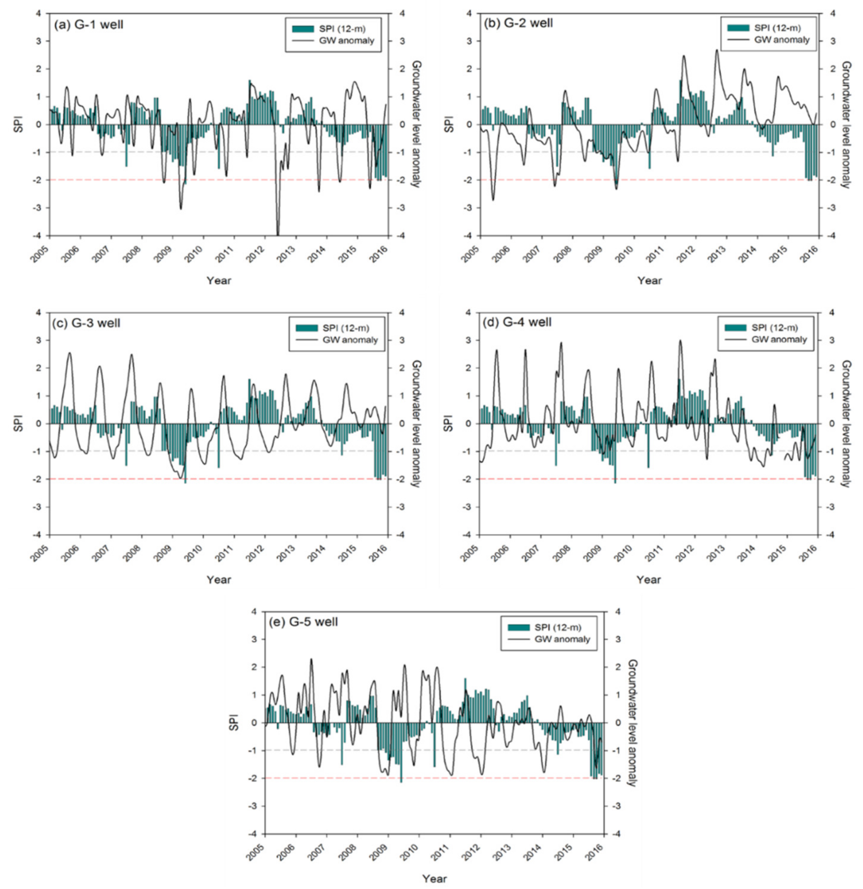
3.4. Groundwater Drought

In this study, drought caused by a lack of precipitation was estimated using the SPI at a time scale of 12 months (SPI-12) for the period 2005–2015 (Figure 6). The periods of 2008–2009 and 2008–2015 experienced severely dry (SPI −1.99 ~ −1.50) to extremely dry (SPI < −2.0) conditions [54]. However, the standardized groundwater level anomaly [57,62,63], as indicated by [(observation–average)/standard deviation], varied among the monitoring wells, probably due to their location in terms of the groundwater flow system, the characteristics of aquifer materials, and the man-made impact of groundwater pumping. If the standardized anomaly dropped below –1, the index indicated groundwater drought conditions. When the water level dropped lower than –2, it was considered to represent extreme groundwater drought.
At G-1, a groundwater drought occurred in 2005–2006 and 2008–2015, (i.e., in 10 of the 11 years, Figure 6), with extreme droughts seen in 2009, 2012–2013, and 2015. At G-2, groundwater drought occurred in 2005–2011, (i.e., 7 of the 11 years), with extreme cases seen in 2005, 2007, and 2009. At G-3, there were drought conditions in 2005–2012, (i.e., 8 of the 11 years), with the worst case occurring in 2009. In G-4, groundwater levels declined below the standard deviation from the mean level in 2005, 2009, and 2014–2015, with the lowest level occurring in 2014. At G-5, there were groundwater drought conditions in 2005–2006, 2008–2011, 2013, and 2015. The lowest water levels in wells occurred in spring, except for G-5, where the late autumn had the lowest water level.
The meteorological droughts due to precipitation deficiency in 2008–2009 and 2015 were not directly reflected by groundwater droughts in the monitoring wells. All five wells only had low water levels under drought conditions at the same time in 2005 and in 2009. The frequency of low water level periods in groundwater was also greater than the frequency of low precipitation periods. In addition, the worst droughts due to precipitation deficiency occurred at different times to the worst groundwater droughts. Thus, water level changes indicated that groundwater droughts occurred due to the complicated impact of both precipitation deficiency and man-made factors, such as groundwater pumping. Therefore, in areas where groundwater is a major source of water supply, groundwater drought estimation using water level changes would be an effective measure to assess drought conditions and their effects on water resources.

3.5. Sustainability Assessment of Groundwater Resources

3.5.1. Groundwater Budget of the MRB

The sustainability of groundwater resources was estimated based on the water budget of the MRB area. We estimated recharge using the SWB method (Figure 7), and the amount of annual recharge in each area was also compared with the amount of groundwater abstraction (Table 3). The SWB modelling results revealed spatial variation in groundwater recharge between the upstream and downstream areas. Generally, upstream areas had a higher recharge than downstream areas, and minimal recharge occurred along the floodplain areas, implying that they were groundwater discharge areas. The results confirmed the groundwater responses to precipitation events at each monitoring well. At G-4 and G-5 in the upstream areas, there were significant relationships between precipitation and the water level response, implying that these wells were located in recharge areas (Table 2, Figure 7). In contrast, the downstream agricultural and urbanized areas (i.e., the locations of G-1 and G-2), have experienced anthropogenic disturbances, such as soil addition and road pavements, resulting in limited recharge from precipitation.
There was almost no change over time in the amount of groundwater abstraction in the MRB, with a mean of about 99 mil m3 yr−1 and a standard deviation of 4.5% of the mean value (www.gims.go.kr; Table 3). Because the proportion of the public water supply in the area increased from 89.3% in 2005 to 97.0% in 2014 (www.wamis.go.kr), this abstraction figure indicates the amount of groundwater utilization that is constantly required in the MRB for agriculture and industry. During 2005–2015, the amount of groundwater abstraction in the MRB varied from 27.4% to 49.7% of the groundwater recharge.
Although the amount of groundwater abstraction remained consistent over the period studied, the reduced recharge due to lack of precipitation could generate significant water level declines in the aquifer [64], causing groundwater drought due to storage deficiency. The impact of groundwater abstraction in wells G-1 to G-3 was analyzed. They were found to have low water levels, with drought conditions occurring in 2005–2006 and 2008–2011. During these years, the mean abstraction to recharge ratio was 39.2%. Thus, based on the temporal water level changes, a groundwater abstraction of 39.2% of the total recharge could be used as a significant drought index for the MRB in terms of groundwater utilization and sustainable management.
Less groundwater recharge could induce a water level decline and a decrease in baseflow discharge to streams and surface waters [64]. In most agricultural fields, farmers are dependent upon either groundwater or the water supply from reservoirs and/or streams. The reduced baseflow discharge will decrease the surface water supply, and subsequently lead to agricultural drought due to a shortage of surface water supply rather than a lack of precipitation. This is an indirect process, with time lags based on the hydrogeologic characteristics of the aquifer.

3.5.2. Groundwater Quality

Groundwater quality is another factor influencing the sustainability of groundwater resources. Unless an adequate water quality is maintained, the water cannot be used as a resource. In this study, we obtained groundwater quality data from the annual reports of K-water and the Ministry of Environment (ME). For each station in the NGMN, water quality was measured by these organizations in the first and second half of the year to determine the ionic composition. We compared the major anions and cations (Table A2, Figure 8) with drinking water standards and found that nitrate nitrogen (NO3-N) was the only variable (major ion) exceeding the relevant water quality standard [65] of 10 mg L−1 in samples from 2009 to 2015. Both shallow alluvial and deep bedrock wells at G-2 had high NO3-N concentrations that exceeded the drinking water standard (> 10 mg L−1) almost every year (Figure 8, Table A2). In addition, through the Groundwater Quality Measurement Network [66], established by the ME, groundwater has been monitored in terms of the vulnerability to contamination based on about 20 parameters (including pH, EC, bacteria, nitrate, chloride, cadmium, arsenic, trichloroethylene (TCE), and tetrachloroethylene (PCE)) two or four times every year. The MRB has a mixture of land uses, including industrial areas, and nitrate, TCE, and PCE pollution was detected in some groundwater samples from the industrial area (Table A3).
The natural background level of NO3-N is less than 3 mg L−1 [67], but 27 of 40 measurements (about 67.5%) had higher levels, indicating nitrate pollution. Three measurements exceeded the drinking water standard of 10 mg L−1 (Figure 8). Comparing the locations of the sites with nitrate levels exceeding thresholds in Figure 8 with the distribution of land use appeared in Figure 2a, the source of nitrate was attributed to agricultural activities from the surrounding farmlands.
Land used for agriculture accounted for 42.0% of the total area 32]. Thus, assuming that nitrate contamination was present in 67.5% of the agricultural area, groundwater recharged from 28.4% of the total area is potentially contaminated by nitrate. Subsequently, the amount of groundwater with an adequate water quality that is available for utilization will be decreased by that proportion. Therefore, the ratio of sustainable groundwater abstraction to recharge could be reduced from 39.2% to 28.1%. This fraction of 11.1% of the groundwater resource could be continuously usable depending on the management and protection measures that are implemented; otherwise, the loss of this groundwater resource is inevitable under present agricultural practices.

4. Implications

In this study, we investigated the natural and man-made drivers of groundwater sustainability, such as climate and groundwater abstraction water quality, respectively, based on time-series monitoring of precipitation and groundwater, and water-quality monitoring data from the wells. The MRB shows a typical landscape of river basin from high mountain areas to lower floodplains, which has groundwater recharged in the upstream discharges in the downstream areas.
Groundwater storage of the top aquifer, where most irrigation wells are tapped into, changes in response to the amount of precipitation. In general, the Monsoon effect had been clear, with large amounts of precipitation in the summer’s wet season and relatively less in the dry season. However, the data from the study area during the last decade showed a precipitation trend of decreasing in the summer and increasing in the dry season. Thus, water resource management techniques should be implemented to adapt to these seasonal and temporal changes.
Groundwater hydrographs from five monitoring wells showed spatial variations in temporal changes. In the wells located within the downstream area, water levels are responsive to cumulative rainfall and groundwater recharge occurring horizontally from upgradient areas. However, wells in the upstream areas are more prone to respond to each individual event, with a fast recharge-and-discharge process. One well in the downstream area exhibits water-level fluctuations due to mixed signals of precipitation and pumping effects, resulting in no trend and a complicated relationship with the recharge–discharge characteristics. Therefore, groundwater resource management should consider not only water levels of the aquifer as a proxy of aquifer storage, but also location of the wells along the groundwater flow system and nearby pumping activities.
In addition, the sustainability of groundwater resources should cover the quantity and the quality together. Wells in the agricultural areas in the MRB show significantly high levels of nitrate, implying the input of surface contaminant through the rainfall infiltration. Consequently, groundwater in this area is exposed to the risk of water quality degradation to contamination. Thus, when the groundwater sustainability is estimated, these negative impacts of water quality should be counted in the groundwater recharge process, resulting in a reduction of the readily-available water resources.

Author Contributions

J.M.L. and N.C.W. conceived and designed the research and wrote the paper; J.M.L. and E.H.K. performed the data collection and analysis and proofread the manuscript.

Funding

This research was funded by the Korea Meteorological Administration (grant number, KMIPA 2015-6090), and the National Research Foundation of Korea (grant number, NRF-2017R1A6A1A07015374).

Acknowledgments

The groundwater and precipitation data for this work were obtained from the National Groundwater Information Management and Service Center (GIMS), Water Management Information System (WAMIS) and the Korea Meteorological Administration (KMA). This paper was published as part of J. Lee’s Ph.D. thesis at Yonsei University, 2018. Authors deeply appreciate the detailed and constructive comments from anonymous reviewers.

Conflicts of Interest

The authors declare no conflict of interest.

Appendix A

Table A1. Summary of the precipitation characteristics recorded at Jeonju station over 11 years.
YearAmount of Rainfall (mm)Rainy DayRainfall Intensity (Wet Season, mm/d)Net P. *
AnnualWet SeasonDry SeasonRatio (Wet/Annual)AnnualWet Season>50 (mm/d)>100 (mm/d)
20051390113026081.3128556220.5401
2006118881537368.6118522115.7169
20071472110636675.2127625117.8533
2008100068331768.3113573012.0-47
2009116484232272.3115465018.373
2010146398447967.3136618116.1451
20111622116845472.0123584220.1582
2012136099236873.0123496020.2257
2013126581844764.7119495016.7199
2014120775645162.6124574013.319
201581433248140.811938008.7-376
Notes: * Net precipitation: precipitation (mm) – evaporation (mm).
Table A2. Chemical composition of groundwater samples reported by Korea Water Resources Corporation (K-Water) from 2009 to 2015 (unit: mg L−1 except pH).
Year.StationpHCaMgNaKClSO4HCO3NO3-N
2009G-1 *7.838.48.821.51.89.50.858.03.1
G-2a7.822.28.519.41.715.638.258.010.3
G-2b6.641.111.920.22.532.246.858.017.2
G-3a6.634.421.99.83.319.831.0152.50.2
G-3b6.632.620.712.05.022.632.0122.05.8
G-4a*6.542.110.313.53.328.113.261.04.9
G-4b*7.113.82.04.31.321.712.3125.15.0
G-5*6.528.67.710.52.85.09.930.54.0
2010G-17.718.54.07.61.212.10.748.84.5
G-2a6.522.610.625.01.820.141.951.99.0
G-2b6.639.711.623.42.726.842.561.016.6
G-3a6.839.227.112.02.926.953.4173.90.3
G-3b7.034.222.914.94.525.441.0128.15.9
G-4a6.536.99.024.22.537.019.897.66.5
G-4b7.239.29.315.02.119.110.7125.14.8
G-57.034.74.39.12.19.722.182.45.5
2012G-17.533.97.716.45.022.613.694.65.5
G-2a6.024.711.627.01.816.437.964.19.9
G-2b6.247.213.926.53.227.939.491.510.6
G-3a6.342.426.812.42.827.847.8164.71.3
G-3b6.536.122.715.34.329.738.0137.37.4
G-4a6.347.013.525.63.548.924.4122.06.0
G-4b *7.142.213.115.72.322.411.5137.30.1
G-56.019.63.87.44.09.115.245.87.1
2013G-1 *7.016.43.88.41.210.60.451.90.1
G-2a6.237.011.623.02.420.439.670.210.0
G-2b6.319.79.823.22.314.133.364.115.0
G-3a6.438.427.011.72.030.053.5167.83.2
G-3b6.633.722.814.63.230.840.5128.15.2
G-4a6.637.810.021.32.037.019.3109.83.1
G-4b7.338.810.115.51.519.513.4134.25.9
G-56.414.72.77.02.66.716.024.45.2
YearStationpHCaMgNaKClSO4HCO3NO3-N
2014G-18.215.73.97.91.410.30.845.83.5
G-2a6.520.210.120.81.811.833.961.08.2
G-2b6.537.312.021.23.319.936.582.416.1
G-3a6.730.720.613.24.225.736.4100.71.6
G-3b6.837.624.411.02.620.354.1134.25.0
G-4a6.539.712.921.82.434.323.5106.86.9
G-4b7.433.611.015.31.515.114.0119.04.1
G-56.313.22.76.32.36.111.221.44.2
2015G-18.114.43.87.91.37.80.554.93.6
G-2a6.523.39.225.41.619.532.361.011.4
G-2b6.639.312.724.82.728.343.767.117.2
G-3a6.736.624.48.02.218.538.0155.61.7
G-3b6.830.822.013.43.228.034.1112.95.2
G-4a6.844.112.021.82.638.322.9106.87.2
G-4b7.639.010.816.81.525.219.5122.05.0
G-56.323.24.721.13.229.119.321.49.3
Notes: *: low charge balance sample (> 10%). a: alluvial shallow aquifer/ b: bedrock deep aquifer. ‘_’ under bar: exceeded drinking water standard of nitrate nitrogen.
Table A3. Chemical composition and average concentrations of groundwater samples from the Water Quality Monitoring Network during 2009–2015.
StationLat.Lng.UseEC (µS/cm)pHBacteria
(population)
NO3-NClTCEPCE1.1.1-TCETolueneEthylbenzene
K-6-c-135°50′53.89″N126°49′3.94″EG151 7.0 23.0 2.7 16.4
K-3-a-135°57′34.35″N126°57′2.64″EG*415 7.0 7.7 51.3
K-3-b-135°57′43.35″N126°59′12.63″EG153 6.5 2.0 4.2 14.6
K-7-d-4-0136° 1′57.38″N127°15′35.12″EG179 7.3 1.4 1.7 5.4
K-7-b-4-0135°59′19.65″N127°12′25.68″EG223 6.7 1.7 3.2 10.2
K-7-e-4-0135°56′14.02″N127° 9′44.02″EG132 7.0 1.7 2.5 13.2
K-7-c-4-0136° 0′28.94″N127°12′19.46″EG239 6.8 5.0 6.2 17.6
K-7-a-1-0135°53′3.81″N127° 9′11.58″EG183 6.8 1.0 2.6 23.3
K-1-e-4-0135°51′44.11″N127° 4′9.32″EG245 6.9 2.0 3.7 17.6
K-1-a-4-0135°48′32.90″N127° 9′18.37″EG387 7.6 1.9 4.3 32.8
K-1-b-1-0135°49′21.64″N127° 8′34.58″EG96 7.5 4.5 2.4 23.2
K-1-d-2-0135°51′13.14″N127° 8′28.87″EG*218 6.8 6.0 16.9
K-1-c-4-0135°46′15.28″N127° 4′52.51″EA237 6.6 4.0 7.8 25.7
FC020135°56′32.56″N127° 7′11.83″EI384 6.9 10.6 9.5
FC020335°56′24.83″N127° 8′1.24″EI255 6.7 18.6 7.3 9.5 0.051 0.006 0.002 0.002
FC020235°56′8.75″N127° 7′46.78″EI324 6.4 4.7 40.2 0.098 0.007 0.002
OC010135°50′52.60″N127° 6′40.85″EG226 7.1 1.0 6.0 23.6
OC010235°50′57.11″N127° 6′55.19″EG456 7.3 24.5 3.1 36.9 0.002 0.001
IC010235°51′48.31″N127° 4′27.38″EG273 7.1 13.0 3.6 20.7 0.002
IC010135°51′34.08″N127° 4′44.99″EG115 7.3 1.1 8.7
OC010335°51′22.35″N127° 6′51.71″EI418 6.7 0.8 23.1
BC010135°51′31.58″N127° 6′9.80″EI417 6.6 2.0 0.6 41.2 0.030 0.013
FC010135°51′21.05″N127° 6′10.34″EG262 7.0 1.1 14.3 0.000
BC010335°51′56.72″N127° 6′20.92″EI493 6.9 5.0 1.0 29.1 0.003
BC010235°51′52.97″N127° 6′10.33″EI522 6.7 6.0 1.7 34.5 0.004 0.001
FC010335°51′51.76″N127° 5′53.32″EI480 6.6 10.0 0.3 23.4 0.001 0.001
FC010235°51′35.99″N127° 5′39.79″EG482 6.9 18.7 5.3 36.8 0.001
IC010335°51′35.97″N127° 4′57.47″EG305 7.1 20.0 4.4 21.4 0.010
FC030135°56′51.10″126°58′32.62″EI475 6.4 8.2 48.9 0.0470.004
FC030235°56′53.16″N126°58′47.79″EI277 6.5 3.8 25.2 0.027 0.040 0.002
FC040235°57′25.29″N127° 0′18.31″EI96 7.0 4.0 0.2 4.2 0.001
FC040335°57′12.95″N127° 0′53.84″EI341 6.6 34.0 5.8 20.7
FC040135°57′21.21″N127° 1′2.40″EI138 6.7 4.0 4.1 9.9 0.007 0.003
GC010135°57′43.25″N127° 1′38.82″EA159 7.0 22.7 2.1 10.3 0.000
GC010235°57′43.25″N127° 1′38.82″EA116 6.7 10.0 1.2 7.7
CC020335°48′2.26″N126°53′12.27″EG393 7.1 12.0 9.4 56.1
CC020235°48′6.75″N126°53′11.95″EG125 7.3 1.4 16.2
Notes: * for drinking. G, general; I, industrial; A, agricultural. Unit: mg/L. ‘_’ under bar, exceeded standard. Blank, below detection limit or not exceeding the water quality standard.

References

  1. Adger, W.N.; Arnell, N.W.; Tompkins, E.L. Successful adaptation to climate change across scales. Global Environ. Chang. 2005, 15, 77–86. [Google Scholar] [CrossRef]
  2. Cioffi, F.; Conticello, F.; Lall, U.; Marotta, L.; Telesca, V. Large scale climate and rainfall seasonality in a Mediterranean Area: Insights from a non-homogeneous Markov model applied to the Agro-Pontino plain. Hydrol. Process. 2017, 31, 668–686. [Google Scholar] [CrossRef]
  3. Karl, T.R.; Trenberth, K.E. Modern global climate change. Science 2003, 302, 1719–1723. [Google Scholar] [CrossRef] [PubMed]
  4. Sheffield, J.; Wood, E.F. Projected changes in drought occurrence under future global warming from multi-model, multi-scenario, IPCC AR4 simulations. Clim. Dynam. 2008, 31, 79–105. [Google Scholar] [CrossRef]
  5. Sheffield, J.; Wood, E.F.; Roderick, M.L. Little change in global drought over the past 60 years. Nature 2012, 491, 435–438. [Google Scholar] [CrossRef] [PubMed]
  6. Di Matteo, L.; Dragoni, W.; Maccari, D.; Piacentini, S.M. Climate change, water supply and environmental problems of headwaters: The paradigmatic case of the Tiber, Savio and Marecchia rivers (Central Italy). Sci. Total Environ. 2017, 598, 733–748. [Google Scholar] [CrossRef] [PubMed]
  7. IPCC. Impacts, Adaptation and Vulnerability Contribution of Working Group II to the Fourth Assessment Report of the Intergovernmental Panel on Climate Change; Cambridge University Press: Cambridge, Cambridgeshire, UK, 2007; p. 976. [Google Scholar]
  8. Oki, T.; Kanae, S. Global hydrological cycles and world water resources. Science 2006, 313, 1068–1072. [Google Scholar] [CrossRef] [PubMed]
  9. Foster, S.; Garduno, H.; Evans, R.; Olson, D.; Tian, Y.; Zhang, W.Z.; Han, Z.S. Quaternary Aquifer of the North China Plain—Assessing and achieving groundwater resource sustainability. Hydrogeol. J. 2004, 12, 81–93. [Google Scholar] [CrossRef]
  10. Esteller, M.V.; Diaz-Delgado, C. Environmental effects of aquifer overexploitation: A case study in the highlands of Mexico. Environ. Manage. 2002, 29, 266–278. [Google Scholar] [CrossRef] [PubMed]
  11. Barnett, T.P.; Pierce, D.W.; Hidalgo, H.G.; Bonfils, C.; Santer, B.D.; Das, T.; Bala, G.; Wood, A.W.; Nozawa, T.; Mirin, A.A.; et al. Human-induced changes in the hydrology of the western United States. Science 2008, 319, 1080–1083. [Google Scholar] [CrossRef] [PubMed]
  12. Milly, P.C.D.; Dunne, K.A. A Hydrologic Drying Bias in Water-Resource Impact Analyses of Anthropogenic Climate Change. J. Am. Water Resour. Assoc. 2017, 53, 822–838. [Google Scholar] [CrossRef]
  13. Mishra, A.K.; Singh, V.P. A review of drought concepts. J. Hydrol. 2010, 391, 204–216. [Google Scholar] [CrossRef]
  14. Van Loon, A.F. Hydrological Drought Explained; Wiley Periodicals, Inc.: Hoboken, NJ, USA, 2015. [Google Scholar]
  15. Karimov, A.; Smakhtin, V.U.; Mavlonov, A.; Borisov, V.; Gracheva, I.; Miryusupov, F.; Djumanov, J.; Khamzina, T.; Ibragimov, R.; Abdurahmanov, B. Managed Aquifer Recharge: The Solution for Water Shortages in the Fergana Valley; International Water Management Institute (IWMI): Colombo, Sri Lanka, 2013; 51p. [Google Scholar]
  16. Lee, J.Y. Environmental issues of groundwater in Korea: implications for sustainable use. Environ. Conserv. 2011, 38, 64–74. [Google Scholar] [CrossRef]
  17. La Licata, I.; Colombo, L.; Francani, V.; Alberti, L. Hydrogeological Study of the Glacial-Fluvioglacial Territory of Grandate (Como, Italy) and Stochastical Modeling of Groundwater Rising. Appl. Sci-Basel 2018, 8, 1456. [Google Scholar] [CrossRef]
  18. Jan, C.D.; Chen, T.H.; Lo, W.C. Effect of rainfall intensity and distribution on groundwater level fluctuations. J. Hydrol. 2007, 332, 348–360. [Google Scholar] [CrossRef]
  19. Kim, K.S.; Lim, T.K.; Park, C.H. Analysis of the Secular Trend of the Annual and Monthly Precipitation Amount of South Korea. J. Korean Soc. Hazard Mitig. 2009, 9, 17–30. [Google Scholar]
  20. Lee, B.; Hamm, S.Y.; Jang, S.; Cheong, J.Y.; Kim, G.B. Relationship between groundwater and climate change in South Korea. Geosci. J. 2014, 18, 209–218. [Google Scholar] [CrossRef]
  21. Park, Y.C.; Jo, Y.J.; Lee, J.Y. Trends of groundwater data from the Korean National Groundwater Monitoring Stations: indication of any change? Geosci. J. 2011, 15, 105–114. [Google Scholar] [CrossRef]
  22. KMA. Abnormal Climate Report 2016; Korea Meteorological Administration: Seoul, Korea, 2016. [Google Scholar]
  23. ME; NIER. Korean Climate Change Assessment Report 2014; Ministry of Environment and National Institute of Environmental Research: Sejong, Korea, 2015.
  24. Choi, G.; Kwon, W.-T.; Boo, K.-O.; Cha, Y.-M. Recent spatial and temporal changes in means and extreme events of temperature and precipitation across the Republic of Korea. J. Korean Geogr. Soc. 2008, 43, 681–700. [Google Scholar]
  25. Yoo, J.; Kwon, H.H.; Kim, T.W.; Ahn, J.H. Drought frequency analysis using cluster analysis and bivariate probability distribution. J. Hydrol. 2012, 420, 102–111. [Google Scholar] [CrossRef]
  26. BGR. Groundwater and Climate Change: Challenges and Possibilities; Bundesanstalt für Geowissenschaften und Rohstoffe (BGR) and Geological Survey of Denmark and Greenland (GEUS): Hannover, Germany, 2008; p. 14. [Google Scholar]
  27. MOLIT; K-Water. Groundwater Annual Report; Ministry of Land, Infrastructure, and Transport (MOLIT) and Korea Water Resources Corporation (K-Water): Daejeon, Korea, 2016; p. 647.
  28. Kiem, A.S.; Austin, E.K. Drought and the future of rural communities: Opportunities and challenges for climate change adaptation in regional Victoria, Australia. Global Environ. Chang. 2013, 23, 1307–1316. [Google Scholar] [CrossRef] [Green Version]
  29. Capri, E.; Civita, M.; Corniello, A.; Cusimano, G.; De Maio, M.; Ducci, D.; Fait, G.; Fiorucci, A.; Hauser, S.; Pisciotta, A.; et al. Assessment of nitrate contamination risk: The Italian experience. J. Geochem. Explor. 2009, 102, 71–86. [Google Scholar] [CrossRef] [Green Version]
  30. Jakobczyk-Karpierz, S.; Sitek, S.; Jakobsen, R.; Kowalczyk, A. Geochemical and isotopic study to determine sources and processes affecting nitrate and sulphate in groundwater influenced by intensive human activity—Carbonate aquifer Gliwice (southern Poland). Appl. Geochem. 2017, 76, 168–181. [Google Scholar] [CrossRef]
  31. Lee, J.M.; Park, J.H.; Chung, E.; Woo, N.C. Assessment of Groundwater Drought in the Mangyeong River Basin, Korea. Sustainability 2018, 10, 831. [Google Scholar] [CrossRef]
  32. MLTM. Mangyeong River Basic Plan; Ministry of Land, Transport and Maritime Affairs (MLTM): Seoul, Korea, 2012. [Google Scholar]
  33. Lee, J.M.; Woo, N.C.; Lee, C.J.; Yoo, K. Characterising Bedrock Aquifer Systems in Korea Using Paired Water-Level Monitoring Data. Water 2017, 9, 420. [Google Scholar] [CrossRef]
  34. Yan, X.; Su, X. Linear Regression Analysis: Theory and Computing; World Scientific: Singapore, 2009. [Google Scholar]
  35. Lanzante, J.R. Resistant, robust and non-parametric techniques for the analysis of climate data: Theory and examples, including applications to historical radiosonde station data. Int. J. Climatol. 1996, 16, 1197–1226. [Google Scholar] [CrossRef]
  36. Mann, H.B. Nonparametric tests against trend. Econometrica 1945, 13, 245–259. [Google Scholar] [CrossRef]
  37. Kendall, M.G. Rank Correlation Methods; Charles Griffin: London, UK, 1975. [Google Scholar]
  38. McCuen, R.H. Modeling Hydrological Change: Statistical Methods; CRC Press: Boca Raton, FL, USA, 2002. [Google Scholar]
  39. Gilbert, R.O. Statistical Methods for Environmental Pollution Monitoring; Van Nostrand Rienhold Company: New York, NY, USA, 1987. [Google Scholar]
  40. Sen, P.K. Estimates of the regression coefficient based on Kendall’s tau. J. Am. Stat. Assoc. 1968, 63, 1379–1389. [Google Scholar] [CrossRef]
  41. Kahya, E.; Kalayci, S. Trend analysis of streamflow in Turkey. J. Hydrol. 2004, 289, 128–144. [Google Scholar] [CrossRef]
  42. Rosenberry, D.O. Unsaturated-zone wedge beneath a large, natural lake. Water Resour. Res. 2000, 36, 3401–3409. [Google Scholar] [CrossRef] [Green Version]
  43. Schicht, R.J.; Walton, W.C. Hydrologic Budget for Three Small Watersheds in Illinois; Illinois State Water Survey, Report on Investigation: Champaign, IL, USA, 1961; p. 40. [Google Scholar]
  44. Demlie, M. Assessment and estimation of groundwater recharge for a catchment located in highland tropical climate in central Ethiopia using catchment soil-water balance (SWB) and chloride mass balance (CMB) techniques. Environ. Earth Sci. 2015, 74, 1137–1150. [Google Scholar] [CrossRef]
  45. Sharda, V.N.; Kurothe, R.S.; Sena, D.R.; Pande, V.C.; Tiwari, S.P. Estimation of groundwater recharge from water storage structures in a semi-arid climate of India. J. Hydrol. 2006, 329, 224–243. [Google Scholar] [CrossRef]
  46. Chenini, I.; Ben Mammou, A. Groundwater recharge study in arid region: An approach using GIS techniques and numerical modeling. Comput. Geosci. 2010, 36, 801–817. [Google Scholar] [CrossRef]
  47. Flint, A.L.; Flint, L.E.; Kwicklis, E.M.; Fabryka-Martin, J.T.; Bodvarsson, G.S. Estimating recharge at Yucca Mountain, Nevada, USA: comparison of methods. Hydrogeol. J. 2002, 10, 180–204. [Google Scholar] [CrossRef]
  48. Healy, R.W.; Cook, P.G. Using groundwater levels to estimate recharge. Hydrogeol. J. 2002, 10, 91–109. [Google Scholar] [CrossRef]
  49. Han, W.S.; Graham, J.P.; Choung, S.; Park, E.; Choi, W.; Kim, Y.S. Local-scale variability in groundwater resources: Cedar Creek Watershed, Wisconsin, USA. J. Hydro-Environ. Res. 2018, 20, 38–51. [Google Scholar] [CrossRef]
  50. Tillman, F.D.; Gangopadhyay, S.; Pruitt, T. Changes in groundwater recharge under projected climate in the upper Colorado River basin. Geophys. Res. Lett. 2016, 43, 6968–6974. [Google Scholar] [CrossRef]
  51. Zhang, J.E.; Felzer, B.S.; Troy, T.J. Extreme precipitation drives groundwater recharge: the Northern High Plains Aquifer, central United States, 1950-2010. Hydrol. Process. 2016, 30, 2533–2545. [Google Scholar] [CrossRef]
  52. Thornthwaite, C.W.; Mather, J.R. Instructions and tables for computing potential evapotranspiration and the water balance: in Publications in Climatology: Centerton, NJ. Lab. Clim. 1957, 10, 185–311. [Google Scholar]
  53. Freeze, R.A.; Cherry, J.A. Groundwater; Prentice Hall: Upper Saddle River, NJ, USA 1979. [Google Scholar]
  54. McKee, T.B.; Doesken, N.J.; Leist, J. The relationship of drought frequency and duration time scales. In Proceedings of the 8th Conference on Applied Climatology, Anaheim, CA, USA, 17–23 January 1993; American Meteorological Society: Boston, MA, USA, 1993; pp. 179–184. [Google Scholar]
  55. Palmer, W.C. Meteorologic Drought; Research Paper, No. 45; U.S. Department of Commerce, Weather Bureau: Washington, DC, USA, 1965. [Google Scholar]
  56. WMO. Standardized Precipitation Index User Guide; WMO-No. 1090; Svoboda, M., Hayes, M., Wood, D., Eds.; WMO: Geneva, Switzerland, 2012. [Google Scholar]
  57. Jaranilla-Sanchez, P.A.; Wang, L.; Koike, T. Modeling the hydrologic responses of the Pampanga River basin, Philippines: A quantitative approach for identifying droughts. Water Resour. Res. 2011, 47, W03514. [Google Scholar] [CrossRef]
  58. Lee, J.Y.; Yi, M.J.; Lee, J.M.; Ahn, K.H.; Won, J.H.; Moon, S.H.; Cho, M. Parametric and non-parametric trend analysis of groundwater data obtained from national groundwater monitoring stations. J. Soil Groundw. Environ. 2006, 11, 56–67. [Google Scholar]
  59. Hirsch, R.M.; Slack, J.R.; Smith, R.A. Techniques of trend analysis for monthly water-quality data. Water Resour. Res. 1982, 18, 107–121. [Google Scholar] [CrossRef]
  60. Eckhardt, K.; Ulbrich, U. Potential impacts of climate change on groundwater recharge and streamflow in a central European low mountain range. J. Hydrol. 2003, 284, 244–252. [Google Scholar] [CrossRef]
  61. Ha, K.; Ko, K.S.; Koh, D.C.; Yum, B.W.; Lee, K.K. Time Series Analysis of the Responses of the Groundwater Levels at Multi-depth Wells According to the River Stage Fluctuations. Econ. Environ. Geol. 2006, 39, 269–284. [Google Scholar]
  62. Asoka, A.; Gleeson, T.; Wada, Y.; Mishra, V. Relative contribution of monsoon precipitation and pumping to changes in groundwater storage in india. Nat. Geosci. 2017, 10, 109–117. [Google Scholar] [CrossRef]
  63. Makokha, G.O.; Wang, L.; Zhou, J.; Li, X.P.; Wang, A.H.; Wang, G.P.; Kuria, D. Quantitative drought monitoring in a typical cold river basin over Tibetan Plateau: An integration of meteorological, agricultural and hydrological droughts. J. Hydrol. 2016, 543, 782–795. [Google Scholar] [CrossRef]
  64. Döll, P.; Mueller Schmied, H.; Schuh, C.; Portmann, F.T.; Eicker, A. Global-scale assessment of groundwater depletion and related groundwater abstractions: Combining hydrological modeling with information from well observations and GRACE satellites. Water Resour. Res. 2014, 50, 5698–5720. [Google Scholar] [CrossRef] [Green Version]
  65. WHO. Guidelines for Drinking-Water Quality., Recommendations, 3rd ed.; World Health Organization: Geneva, Switzerland, 2004. [Google Scholar]
  66. ME. Groundwater Quality Measurement Network Operating Result Report; Ministry of Environment: Sejong, Korea, 2009–2015. [Google Scholar]
  67. MacLeod, C.L.; Barringer, T.H.; Vowinkel, E.F.; Price, C.V. Relation of Nitrate Concentrations in Ground Water to Well Depth, Well Use, and Land Use in Franklin Township, Gloucester County, New Jersey, 1970–85; Water-Resources Investigations Report 94-4174; U.S. Geological Survey: West Trenton, NJ, USA, 1995. [Google Scholar]
Figure 1. (a) A map depicting the catchment boundary and locations of each monitoring station in the Mangyeong River Basin (MRB), Korea, (b) lithologic profiles and well descriptions (adapted from Lee et al. [31]).
Sustainability 11 01486 g001
Figure 2. Gridded data used in a soil water balance (SWB) model assessment of the MRB: (a) land use (land cover classification), (b) hydrological soil group based on infiltration rate, (c) groundwater flow direction, and (d) available water capacity.
Sustainability 11 01486 g002
Figure 3. Changes in the amount of precipitation during the wet (June–September, blue circle and dashed line) and dry (October–May, red circle and dashed line) seasons, based on data recorded at the Jeonju weather station from 2005 to 2015.
Sustainability 11 01486 g003
Figure 4. Groundwater hydrographs of the five monitoring wells (a–e) and daily precipitation (f) in the MRB for the period 2005–2015.
Sustainability 11 01486 g004
Figure 5. Representative patterns of water level fluctuations and cumulative precipitation at monitoring wells in the MRB, Korea: (a) G-1, (b) G-2, (c) G-3, (d) G-4, and (e) G-5.
Sustainability 11 01486 g005
Figure 6. Monthly trends in the groundwater standardized precipitation index at a time scale of 12 months (SPI-12) in the MRB, Korea: blue and red lines indicate guidelines for index values of −1 and −2.
Sustainability 11 01486 g006
Figure 7. Estimated groundwater recharge using the SWB model in the MRB for the period 2005–2015.
Sustainability 11 01486 g007
Figure 8. Spatial distribution of the average concentrations of nitrate-nitrogen in groundwater samples in the MRB.
Sustainability 11 01486 g008
Table 1. Hydrogeological properties and statistics on water level fluctuations at the five wells.
WellAquiferAquifer Type aWell Depth (m)Water Level (m)Mean Depth to Water (m) cHydraulic Conductivity (m/day) dSoil Type
Mean (a.s.l.) bAve. Annual Change
G-1Biotite granite (Bedrock)SC7013.671.580.550.34Loam
G-2Gneissic granite (Alluvial)UC1229.951.962.750.01Sandy loam
G-3Schistose granite (Alluvial)ND159.451.696.600.23Loam
G-4Biotite granite (Alluvial)SC1223.791.173.770.01Sandy loam
G-5Volcanic rocks (Bedrock)UC7068.551.322.620.25Loam
Notes: a Aquifer type determined by Lee et al. [33]: UC, unconfined aquifer; SC, semi-confined aquifer; ND, not determined. b a.s.l. means above sea level. c Average value for 11 years (2005–2015). d Hydraulic conductivity evaluated by pumping test (GIMS, www.gims.go.kr).
Table 2. Results of trend (parametric and non-parametric) and correlation analyses of rainfall and groundwater data obtained from monitoring stations in the Mangyeong River Basin (MRB), Korea.
Observation Well Trend AnalysesCorrelation Coefficients a
Linear RegressionM-K Test *Sen’s Test *Lag-time
(day)
WL and
Rainfall
Period
DMDMDMWet SeasonDry Season
G-1--NTNTNTN00.0860.366 *−0.162
G-2++PPPP-−0.035−0.199−0.233 *
G-3++PNTPP00.454 **0.1640.124
G-4--NNNN00.750 **0.721 **0.268 **
G-5--NNNN00.599 **0.722 **0.437 **
Rainfall--NTNTNTNT----
Notes: D: daily data, M: monthly data. a: monthly water level (WL) data and precipitation data. +/−: increasing/decreasing trend. P, N and NT denote positive, negative and no trend, respectively. *: significant at p < 0.05, **: significant at p < 0.01
Table 3. Estimated groundwater annual recharge and the amount of abstraction from 2005 to 2015 in the Mangyeong River Basin (MRB), Korea.
YearMean Recharge Rate (mm)Amount of Abstraction (1)Calculated Recharge (2)Abstraction to Recharge Ratio (%) (3)
2005163.1101,669,325260,908,80039.0
2006141.093,147,785225,552,00041.3
2007229.695,551,861367,385,60026.0
2008120.195,584,978192,227,20049.7
2009119.994,772,404191,820,80049.4
2010215.496,955,614344,627,20028.1
2011233.9102,676,289374,294,40027.4
2012229.1103,082,918366,572,80028.1
2013175.3104,575,749280,416,00037.3
2014173.5104,869,683277,571,20037.8
201586.4-138,176,000-
Mean171.599,288,661274,504,72736.2
Notes: (1) measured data obtained from the National Groundwater Information Center (GIMS) (www.gims.go.kr) (unit: m3 yr−1), (2) calculated data using a simulation from the soil water balance (SWB) model (unit: m3 yr−1), (3) ratio = (1)/(2)

