Abstract
Recognizing the change in regulation of energy consumption may help China to control total energy consumption and realize sustainable development during rapid urbanization and industrialization. This paper re-examined the trans-provincial convergence of per capita energy consumption from 1990–2015 using five different kinds of methods for 30 Chinese provinces. Results show that per capita energy consumption across Chinese provinces was convergent. However, the results obtained by different methods were slightly different. First, it shows a weak beta-unconditional convergence during the entire period, as well as a significant beta-unconditional and conditional piecewise convergence from 1990–2000 and 2001–2015. Second, it shows a significant sigma-convergence indicated by a marked decrease in the standard deviation of logarithm (SDlog) and the coefficient of variation (CV). Third, the kernel density curve became narrower during 1990–2015, indicating that the per capita energy consumption of each Chinese province converged to a common equilibrium level, which was about 80% of the national average. Fourth, the intra-distributional mobility index implied a weak gamma-convergence. Fifth, the first difference of DF (Dickey-Fuller), ADF (Augmented Dickey-Fuller), and PP (Phillips-Perron) unit-root tests all suggested a stochastic convergence. On the whole, the results from this paper contribute to a more in-depth understanding of the status quo of per capita energy consumption in China, as well as a meaningful implication for differentiated energy policies and sustainable development strategies.
1. Introduction
China, which is the most populous country and the largest energy consumer in the world, is currently facing energy scarcity and environmental degradation due to the increasing energy demands of rapid urbanization and industrialization [1,2,3,4,5,6,7,8]. In 1990, China’s total population was 1143.33 million. It steadily increased to 1374.62 million in 2015, with an average annual growth rate of 0.74%. Meanwhile, the total energy consumption of China increased from 953.84 million tons of coal equivalent (Mtce) in 1990 to 4021.64 Mtce in 2015, with an average annual growth rate of 5.92%. However, the average annual growth rate of China’s energy consumption fluctuated greatly. It was 3.99% during the period from 1990–2000, reaching up to 9.32% during the period from 2000–2010, and falling to 3.20% during the period from 2010–2015. Accordingly, per capita energy consumption in China increased unstably from 0.8343 tce in 1990 to 2.9256 tce in 2015, with an average annual growth rate of 5.15%. As China has achieved great successes in population control, the future energy demand may depend chiefly on per capita energy consumption [9,10]. However, per capita energy consumption in China’s different provinces is various due to the differences in economic development levels and energy efficiency [4,5,9,10,11]. If the gap among Chinese provinces tends to increase, it may cause injustice and welfare loss, and affect the overall energy efficiency. Otherwise, there may be a trans-provincial convergence, i.e., per capita energy consumption in relatively high provinces tends to grow slower or decrease faster, while provinces with lower initial per capita energy consumption will experience more rapid growth, eventually catching up to provinces with higher per capita energy consumption. Therefore, it is easier to implement strict regulations on energy consumption and environment protection in provinces with higher per capita energy consumption. However, for the provinces with relatively low per capita energy consumption, relatively loose policy to control energy consumption had better be adopted. In a theoretical manner, to realize convergence, it may substantially compress the reduction of China’s energy consumption while equalizing per capita energy consumption across provinces gradually.
Convergence was originally used in the economic field to judge the state of economic growth [12]. As it lies behind economic policy, a large number of empirical studies on economic convergence have been carried out [13]. Subsequently, it was gradually applied to energy-related indicators, such as energy consumption, energy intensity, carbon dioxide emissions, electricity consumption, and electricity intensity [11,14,15,16,17,18,19,20,21,22,23]. However, numerous analyses of energy convergence using various approaches and at different scales have obtained mixed results. Among them, some empirical analyses show convergence while some show divergence. For instance, Liddle [15] used two new large datasets and four econometric measures to confirm the existence of convergence by studying the energy intensity of over 100 countries during the period from 1971–2006, but pointed out that there were geographical differences in convergence, e.g., OECD countries, Eurasian countries, and sub-Saharan African countries showed convergence, while Latin American, Caribbean, Middle Eastearn, and North African countries presented no convergence. Herrerias [16] used a weighted distribution dynamics approach to investigate the convergence of energy intensity in 83 countries during the period from 1971–2008, and found that developing countries may converge at higher ratios, while developed countries may fall into at least two convergence clubs, i.e., the lowest levels and the higher levels of energy intensity. Mulder and Groot [18] used new and unique data to evaluate the structural change and convergence of energy intensity across 18 OECD countries and 50 sectors during the period from 1970–2005, and found evidence for the hypothesis that across sectors, lagging countries are catching-up with leading countries, with rates of convergence that are on average higher in services than in manufacturing. Meng et al. [19] employed newly developed LM (Lagrange Multiplier) and RALS-LM (Residual Augmented Least squares - Lagrange Multiplier) unit root tests with allowance for two endogenously determined structural breaks to examine the convergence of per capita energy consumption among 25 OECD countries during the period from 1960–2010 and found that per capita energy consumption of the OECD countries was significantly convergent. Mishra and Smyth [20] used the panel KPSS (Kwiatkowski, Plillips, Schmidt and Shin) stationarity test and panel Lagrange multiplier (LM) unit root test to confirm the convergence in per capita energy consumption among ASEAN (Association of Southeast Asian Nations) countries during the period from 1971–2011. However, Mohammadi and Ram [23] used several parametric and non-parametric approaches to explore the convergence in per capita energy consumption across the US states during the period from 1970–2013, and concluded that there seemed to be a lack of convergence of per capita energy consumption across the United States. In short, empirical studies related to energy indicators rather than theoretical explanations generally cause the debates in the related literature. The convergences of different countries and regions are controversial.
As for energy-related indicators in China, more studies have been carried out on the convergence of carbon dioxide emissions, energy intensity, and electricity intensity [5,11,24,25,26,27,28]. For instance, Jiang et al. [5] used unconditional and conditional beta convergence, sigma convergence, and kernel density analysis to investigate the convergence of energy intensity in provincial China during the period from 2003–2015, and found that the omission of spatial spillovers underestimated conditional beta convergence. Huang and Meng [11] developed the spatial convergence model with spatiotemporal effect specification for urban China, and found that per capita carbon dioxide emissions in China increased and converged during the period from 1985–2008. Herrerias and Liu [24] used several unit root tests to explore the stochastic convergence of electricity intensity across Chinese provinces, and found that most Chinese regions converged but a few regions diverged. Wang et al. [25] used the log t-test to investigate the convergence of carbon dioxide emissions in China during the period from 1995–2011, and found evident convergence to three steady state equilibriums at the provincial level while divergence was found at the country level. Zhao et al. [26] used a spatial dynamic panel data model to investigate the convergence of carbon dioxide emission intensities in provincial China during the period from 1990–2010, and found that carbon dioxide emission intensities were convergent across provincial China. Wu et al. [27] employed a continuous dynamic distribution approach and found the convergence of per capita carbon dioxide emissions by panel data of 286 cities in China during the period from 2002–2011. Yu et al. [28] used an environmental performance index method and some convergence models to explore the carbon emissions intensity convergence of 24 industrial sectors in China during the period from 1995–2015, and found a beta-conditional convergence. However, within the scope of our literature retrieval through Web of Science, we only found three studies on the convergence of per capita energy consumption in China. Herrerias et al. [3] used the club convergence analysis to confirm the effect of the regional concentration of economic activity on per capita residential energy consumption across Chinese regions during the period from 1995–2011. Hao et al. [9] investigated the existence of convergence in per capita energy consumption across Chinese provinces with the possible breakpoints during the period from 1985–2012, using static and dynamic regression methods and Chow tests. Hao and Peng [10] employed spatial dynamic econometric models to study the convergence of per capita energy consumption across Chinese provinces during the period from 1994–2014, indicating that there were both unconditional and conditional beta-convergences. In order to contribute to a more in-depth understanding of the status quo of per capita energy consumption in China, we re-examined the convergence of per capita energy consumption across Chinese provinces using five different kinds of methods given by Mohammadi and Ram [23], including beta-convergence, sigma-convergence, kernel density estimation, gamma-convergence, and stochastic convergence. The overall scenario seems to be a meaningful implication for China’s differentiated energy policies and sustainable development strategies.
The rest of the paper is structured as follows. Section 2 describes the data and different methodologies for the convergence of per capita energy consumption across 30 Chinese provinces. In Section 3, we present the empirical results and analysis. In Section 4, we draw our conclusions and explore some policy implications.
2. Materials and Methods
2.1. Data Sources
In this study, we used provincial panel data of China’s 30 provincial-level administrative units (except for Tibet, Hong Kong, Macao, and Taiwan) during the period from 1990–2015. The annual data related to population and energy consumption were obtained from the China Statistical Yearbook [29] and China Energy Statistical Yearbook [30] which are openly published by the National Bureau of Statistics of China (NBSC) every year. The meteorological data used in this paper came from the database of the surface meteorological monthly report received by 194 basic datum stations in China’s Meteorological Bureau during the period from 1990–2015, which can be obtained on the website http://data.cma.cn.
2.2. Beta-Convergence
Beta-convergence is widely used for regional convergence. It has two basic forms, including unconditional convergence and conditional convergence [23]. Specifically, unconditional convergence assumes that all convergent regions have identical basic characteristics and growth paths, and all of them may converge to a common equilibrium level. The form of unconditional convergence is written as follows:
where E0 and Et are per capita energy consumption in the initial year and in year t, i is the ith province, and u is the random error terms. The presence of convergence would imply a significant negative sign on b, suggesting that if the initial per capita energy consumption is lower, the growth rate will be higher. However, if the initial per capita energy consumption is higher, the growth rate will be lower.
The conditional convergence considers that all convergent regions have different basic characteristics and growth paths. Therefore, some main influencing factors are introduced as the conditional variables for Equation (1). In that context, cooling-degree-days (C) and heating-degree-days (H) may affect per capita energy consumption in each province. Thus, the form of conditional convergence is written as follows:
where C0i is the cooling-degree-days in the initial year in the ith province. It is the accumulation degree of the daily mean temperature above the base temperature in a year [31,32,33]. H0i is the heating-degree-days in the initial year in the ith province. It is the accumulation degree of the daily mean temperature below the base temperature in a year [31,32,33]. The values of the cooling and heating-degree-days for a year is defined as follows:
where Nd is the number of days in a year; Ti is the daily average temperature; Tb is the base temperature; if the average daily temperature is higher than the base temperature, γd is 1, otherwise it is 0. Specifically, the base temperature for the cooling and heating-degree-days varies across countries/regions depending on many socio-economic and eco-environmental factors [31,32,33]. The Ministry of Housing and Urban–Rural Construction of the People’s Republic of China released The Design Standard for Energy Efficiency of Residential Buildings in Hot Summer and Cold Winter Zones (JGJ134-2010) in 2010, and set the base temperature at 26 °C and 18 °C, respectively, when calculating the values of the cooling- and heating-degree-days [34]. Therefore, we used them in the calculation.
2.3. Sigma-Convergence
Although beta-convergence has been widely used, it is a necessary but not a sufficient condition for regional convergence [23,35]. Moreover, beta-convergence can only be used to analyze the state of a certain period but cannot analyze the unbalanced situation during this period [32]. However, sigma-convergence can show the changes of horizontal differences and the dynamic process of regional growth imbalance over time. Some scholars have adopted different indexes to calculate sigma-convergence [15,36]. This paper used both the standard deviation of logarithm (SDlog) and the coefficient of variation (CV). Specifically, the standard deviation of logarithm (SDlog) is expressed as follows:
where Eit is per capita energy consumption in the ith province in period t; n is the number of Chinese provinces.
The coefficient of variation (CV) is expressed as follows:
where Ei is per capita energy consumption in the ith province; Ē is the average value; S is the standard deviation; n is the number of Chinese provinces.
2.4. Kernel Density Estimation
The parameter estimations of beta-convergence and sigma-convergence, which need to assume that the data conform to a specific distribution, often bring a large gap between the basic assumption and the practical physical model. However, as a non-parametric way, the kernel density estimation only uses the information of the sample data to avoid influence of the prior knowledge of human subjectivity, by looking at the shapes of the distribution of histograms [15,37]. Therefore, the kernel density estimation can be proposed to supplement the beta-convergence and the sigma-convergence. By contrast with histograms in different periods, the kernel density estimation can be endowed with properties such as smoothness or continuity by using a suitable kernel. The universal kernel density estimation is defined as follows:
where K is the kernel function, which is essentially a weighting function; Kh(x) = K(x/h)/h and h > 0; h is a smoothing parameter called the bandwidth; n is the number of samples.
Specifically, a range of kernel functions are commonly used, such as Gaussian, Epanechnikov, uniform, triangular, biweight, triweight, and normal kernel function [38]. The Epanechnikov kernel is optimal in a mean square error sense, and the loss of efficiency is small for the kernels listed previously [39]. Accordingly, the Epanechnikov kernel function was adopted in our study:
where I is an explicit function; when the condition in the parentheses is true, it equals to 1; otherwise it equals to 0.
As for the bandwidth h, when it is larger, the probability of samples distributed around the x is more significant, and the estimated function fh^(x) means more smoothness but it expands the deviation. Therefore, selection of bandwidth is critical for the practical estimation of kernel density function. There are a lot of methods to approximate the optimal bandwidth, such as ROT (rule of thumb), UCV (unbiased cross-validation), and STE (solves the equation) [40]. In this study, we use Silverman’s rule-of-thumb [41] to obtain the optimal bandwidth. The equation of the optimal bandwidth h0 is as follows:
where Sx is the standard deviation (SD) of the samples; n is the number of the samples.
2.5. Gamma-Convergence
By using gamma-convergence, we can determine whether the provinces with the highest and lowest per capita energy consumption remain unchanged in a certain period through the mobility of internal distribution [15,23,42]. The index of rank concordance ranges from 0 to 1. The closer the index is to 0, the larger the range of mobility within the distribution. According to Liddle’s research [15], the gamma-convergence index is as follows:
where R(E)it is the rank of the ith province’s per capita energy consumption in period t; R(E)i0 is the rank of the ith province’s per capita energy consumption in the initial period (year); Variance (R) is the variance of the samples.
2.6. Stochastic Convergence
Stochastic convergence is based on the assumption that there is no convergence if the impact of the variable relative to the sample average persists [21,43]. Therefore, it is necessary to test the existence of the unit-root. The original hypothesis is to reject the existence of unit-root, i.e., the sequence is stable, which means that the series of shocks do not continue and there is a stochastic convergence. If the test does not reject the existence of the unit-root, the sequence is non-stationary, which indicates the existence of persistent shocks and the lack of stochastic convergence. Test of stochastic convergence by unit-root test may be represented via panel data and/or univariate time-series. For instance, Mohammadi and Ram [23] used both the panel unit-root test and the univariate time-series; Hao et al. [9], Hao and Peng [10], and Aldy [36] used the panel unit-root test; and Meng et al. [19], Mishra and Smyth [20], Fallahi [21], Herrerias and Liu [24], and Payne et al. [44] used the univariate time-series. Each kind of unit-root test method has its advantages and shortcomings [21,44]. In the time-series framework, convergence of per capita energy consumption of each spatial unit toward a benchmark spatial unit is tested by the unit-root tests (i.e., testing unit-root in the log relative per capita energy consumption of each spatial unit to the benchmark spatial unit). The benchmark spatial unit may be another spatial unit or the average sample [21,44]. Thus, we can test the stochastic convergence for each province of China using the univariate time-series from 1990–2015. However, for simplicity, we used China as a spatial unit and the average sample of 30 Chinese provinces as a benchmark. The equation is as follows:
where yt is the relative per capita energy consumption of China in time t; Et is per capita energy consumption of China in time t; Eit is per capita energy consumption in the ith province in time t; and n is the number of Chinese provinces.
In this paper, the unit-root test of China’s relative per capita energy consumption from 1990–2015 was carried out by EViews 9. In the test, some frequently-used unit-root test methods, including the DF (Dickey-Fuller) and ADF (Augmented Dickey-Fuller) tests proposed by Dickey and Fuller [45], and the PP (Phillips-Perron) unit-root test proposed by Phillips and Perron [46] were adopted. Generally, if the relative per capita energy consumption defined above follows a stationary process, it means a stochastic convergence [44]. Therefore, according to the above unit-root test methods, if the original time-series are non-stationary, the first or second difference may be used [45,46]. If the statistical value is less than the critical value, the original hypothesis will be accepted. Otherwise, the original hypothesis will be rejected. Finally, comparison among these three kinds of test results and the results obtained from the other four different kinds of methods may improve the reliability of the conclusion.
3. Results
3.1. Descriptive Statistics
Table 1 provides a brief description of statistics on per capita energy consumption in Chinese provinces for every five years during the period for 1990–2015. First, there was a substantial increase in the mean of per capita energy consumption across Chinese provinces, which was 0.8476 tce in 1990 to 3.2541 tce in 2015. Secondly, the standard deviation (SD) increased significantly from 0.6232 in 1990 to 1.6936 in 2015, indicating that the gap between the average per capita energy consumption of the provincial level continued to expand. However, considering the improvement of the overall level of energy consumption, the coefficient of variation (CV) was used to eliminate the influence of the measurement dimension, and then the overall trend declined from 0.7352 in 1990 to 0.5204 in 2015, indicating the possibility of convergence.

Table 1.
Descriptive statistics of per capita energy consumption in China (ton of coal equivalent (tce)).
Figure 1 shows per capita energy consumption in 1990 (the initial year) and 2015 (the latest year), as well as the annual growth rate over the sample period. It suggests that provinces such as Beijing, Shanghai, and Tianjin have the lowest annual average growth rate and the highest initial consumption levels, while provinces such as Hainan, Guangxi, and Jiangxi have the highest annual average growth rate and the lowest initial consumption levels. It also indicates that China’s per capita energy consumption is likely to converge. However, it needs to be further verified by quantitative methods.
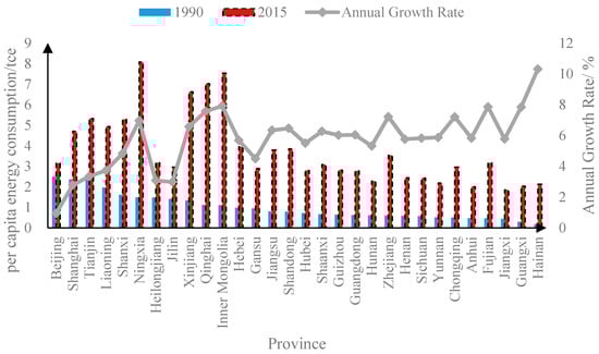
Figure 1.
Per capita energy consumptions and average annual growth rate across Chinese provinces during 1990–2015.
3.2. Test of Beta-Convergence
As for the unconditional beta-convergence, we first calculated the results of the overall stage during the period from 1990–2015 in Table 2. As the regression coefficient b was −0.002, which was a negative value, it conforms to the convergence trend predicted in the above description. However, the p-value was 0.928, which is larger than 10%. The coefficient of determination (R2) was close to zero. Taken together, the goodness of fit was very small and the linear relationship in this period was not significant. Subsequently, according to the characteristics of data distribution over time, we found that per capita energy consumptions in China and most provinces increased sharply from 2000. Therefore, we calculated the results of the piecewise stages during the periods from 1990–2000 and 2001–2015. It shows that the coefficient of determinations (R2) were 0.361 and 0.555, respectively, and the regression coefficients were both negative and both significant at the 5% level. Therefore, in these two stages, China’s per capita energy consumption presents an unconditional beta-convergence with high goodness of fit. Moreover, from the regression coefficients, which were −0.181 and −0.086, respectively, it is seen that the convergence rate from 1990–2000 was relatively fast while that from 2001–2015 was relatively low.
Table 2.
Parameter estimation of beta-convergence in per capita energy consumption in provincial China during 1990–2015.
As for the conditional beta-convergence, the results of the overall stage during the period from 1990–2015 in Table 2 show that the regression coefficient b was positive and the p-value was larger than 10%. The coefficient of determination (R2) was 0.043. It indicates that the linear relationship in the overall stage was not significant or with poor goodness of fit, and the climate conditions may not affect the convergence of per capita energy consumption across provincial China. However, the regression coefficient b was negative and significant at the 10% level during the period from 1990–2000, suggesting a weak conditional beta-convergence. The regression coefficient b was negative and significant at the 5% level during the period from 2001–2015, suggesting a strong conditional beta-convergence. Considering the impact of climate conditions, per capita energy consumption in Chinese provinces also converges in stages, and the impact of climate conditions during the period from 1990–2000 was a little greater than that during the period from 2001–2015.
3.3. Test of Sigma-Convergence
Figure 2 shows the standard deviation of logarithm (SDlog) and the coefficient of variation (CV) of per capita energy consumption across 30 Chinese provinces each year from 1990 to 2015. It is seen that there was an obvious downward trend during the entire period. The SDlog declined from 0.2664 in 1990 to 0.1768 in 2015, while the CV declined from 0.6130 in 1990 to 0.4541 in 2015. Obviously, both of them changed the most suddenly around 2000, which also indicates that a piecewise convergence may have existed during the periods from 1990–2000 and 2001–2015. Moreover, the variation trends of SDlog and CV were similar, i.e., they declined rapidly during the period from 1990–1994, fluctuated slightly during the period from 1994–2001, declined rapidly during the period from 2001–2010, and increased slightly after 2010. It suggests that there was a sigma-convergence as a whole. Meanwhile, the sigma-convergence was more significant during the periods from 1990–1994 and 2001–2010 than in other stages.
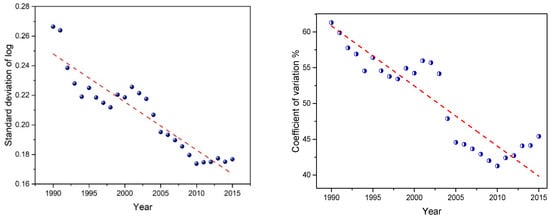
Figure 2.
Sigma (standard deviation of logarithm (SDlog) and the coefficient of variation (CV)) convergence in per capita energy consumption across Chinese provinces, 1990–2015.
Table 3 describes the linear parameters in regression analysis for the standard deviation of logarithm (SDlog) and the coefficient of variation (CV) across 30 Chinese provinces. It is seen that the regression coefficients are −0.0032 and −0.7758 respectively and both negative, and the p-values both indicate a significance at 1% level. Therefore, we can also conclude that there is a significant sigma-convergence in per capita energy consumption across 30 Chinese provinces during the period of 1990–2015.
Table 3.
Estimated linear parameters of sigma-convergence in per capita energy consumption in provincial China, 1990–2015.
3.4. Results of Kernel Density Estimation
Figure 3 shows the kernel density plots using the ratio of per capita energy consumption to the national average as the horizontal ordinate for every five years during the period from 1990–2015. First, we can see that all four plots maintain a unimodal distribution, and the corresponding horizontal ordinates of the peaks are all around 0.8. It indicates that per capita energy consumption in most Chinese provinces was close to 80% of the national average. Second, the corresponding longitudinal coordinates of the peaks became larger during the period from 1990–2015, i.e., it was less than 0.8 in 1990, around 0.9 in 2000, around 1.1 in 2010, and around 1.2 in 2015. It indicates that per capita energy consumption in more and more Chinese provinces was close to 80% of the national average. Finally, the curve of density distribution gradually became narrower from 1990 to 2015. It indicates that provinces in which per capita energy consumption was lower than 80% of the national average had a higher growth rate so that they approached the peak rapidly, while provinces in which per capita energy consumption was higher than 80% of the national average had a slower growth rate so that they departed from the peak slowly. In short, the gap of per capita energy consumption among Chinese provinces reduced during the period from 1990–2015, indicating an obvious convergence.
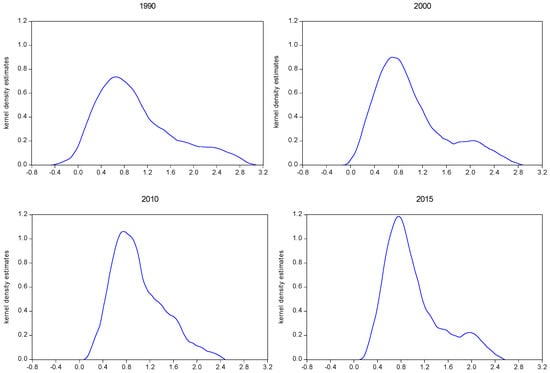
Figure 3.
The kernel density estimation of per capita energy consumption across Chinese provinces, 1990–2015.
3.5. Test of Gamma-Convergence
Figure 4 reveals gamma-convergence by the intra-distribution mobility index for each year from 1990 to 2015. The plot shows a significant negative slope. However, the decline in the vertical axis of the index is very small. It starts from 1.00 in 1990, and remains above 0.94 in 2015. It indicates very little change in the rankings from the initial year. The decline of the index was both smaller than that for per capita energy consumption across US states during the period from 1970–2013 as shown by Mohammadi and Ram [23], and that for energy intensity in OECD countries as shown by Liddle [15] from 1960 to 2006, which was interpreted as having little effect on the rankings. Therefore, it may be indicated as a weak gamma-convergence in terms of changes in the ranks of Chinese provinces.
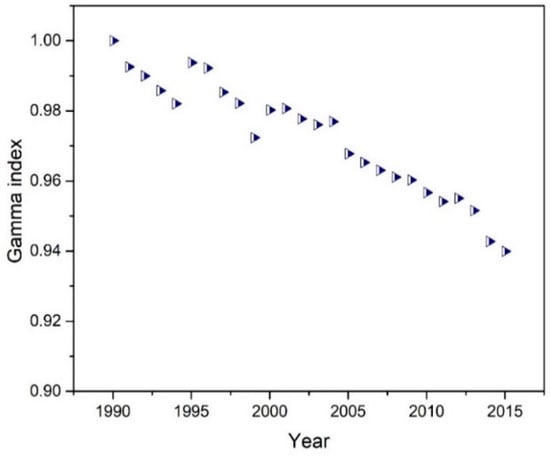
Figure 4.
Gamma-convergence (intra-distributional mobility) in per capita energy consumption across Chinese provinces, 1990–2015.
3.6. Test of Stochastic Convergence
Table 4 shows the DF, ADF, and PP unit-root test results for several lag lengths based on the panel data of per capita energy consumption across 30 Chinese provinces during the period from 1990–2015. As seen in Table 4, the DF test statistic for relative per capita energy consumption (yt) was −2.273, which was smaller than the 5% critical value. The p-value was 0.0322, which was smaller than 5%. It indicates that the existence of a unit-root was rejected and the sequence was stationary. However, the ADF and PP test statistics for relative per capita energy consumption (yt) were both larger than any critical value and the p-values were both larger than 10%. It indicates that the existence of a unit-root was accepted and the sequence was non-stationary. The first differences of relative per capita energy consumption (∆yt) show that the test statistics were all smaller than any critical value and the p-values were all smaller than 1%. It indicates that the sequence of the first difference was stationary at the 1% significance level.
Table 4.
Unit-root tests on relative per capita energy consumption across Chinese provinces during 1990–2015.
In short, the three kinds of methods for the unit-root test all support the stationary of relative per capita energy consumption after the first difference. It means that there is a stochastic convergence. However, the original time-series are both non-stationary in the ADF and PP unit-root test. It means that there may exist persistent shocks or structural breaks which make the data non-stationary. Through data difference, the series of shocks do not continue and all become stationary. It means that there may exist persistent shocks or structural breaks which can be eliminated by data difference. This result accords with the characteristics of data distribution over time, as well as the results of beta and sigma-convergence test.
4. Conclusions and Policy Implications
This paper used five different kinds of methods to explore the convergence of per capita energy consumption across 30 Chinese provinces during the period from 1990–2015, providing a verification and supplement of the methods in the convergence literature, as well as a scientific basis for China’s relevant energy policies. The following main conclusions and policy implications were obtained:
- (1)
- Our predominant finding is that per capita energy consumption across Chinese provinces was convergent during the study period. It means that provinces with a higher initial consumption level have lower growth rates of per capita energy consumption, while provinces with lower initial consumption levels have higher growth rates, so that the gap of per capita energy consumption among Chinese provinces gradually narrows. It seems that per capita energy consumption of each Chinese province converges to a common equilibrium level, which is about 80% of the national average. Therefore, the Chinese government could formulate differentiated and targeted policies for different provinces to control energy consumption [47,48]. Specifically, for the provinces in which per capita energy consumption is lower than 80% of the national average, the energy control target could be relatively loose so that the necessary demand of energy consumption for the economic development could be satisfied. However, for the provinces in which per capita energy consumption is higher than 80% of the national average, strict regulations on energy consumption could be conducted because they have great potentials to reduce energy consumption according to the rules of convergence.
- (2)
- The results obtained by different methods were slightly different. It shows a weak beta-unconditional convergence during the entire period, as well as a significant beta-unconditional and conditional piecewise convergence during the periods from 1990–2000 and 2001–2015. The sigma-convergence was significant during the entire period indicated by a marked decline in the standard deviation of logarithm and the coefficient of variation, but it was more significant during the period from 1990–1994 and 2001–2010 than in other stages. The kernel density curve became narrower during the period from 1990–2015, indicating a significant convergence. The intra-distributional mobility index implies a weak gamma-convergence, which means the gap of per capita energy consumption among Chinese provinces was lessened but the ranks of per capita energy consumption across Chinese provinces had little change. The first difference of DF, ADF, and PP unit-root tests suggest a stochastic convergence. In short, the significances of convergence seem a little inconsistent in different periods and different methods. Therefore, it is necessary to real-time monitor the status quo of per capita energy consumption across Chinese provinces, and adjust energy policy and the corresponding development strategy in time.
- (3)
- As the convergences detected by the five methods are not all strong, we may consider that the convergence is relatively low. It suggests that the demand for energy consumption in China is still huge. To effectively control the rapid growth of energy consumption, the current economic development pattern and urbanization mode that rely heavily on natural resources and ecological environment [49,50,51,52] should be adjusted. For instance, China should promote the development of a low-carbon economy by accelerating the development of tertiary industry and industries with new technology and high added-values. Meanwhile, energy-intensive firms and industries in the secondary industry should be gradually closed down to adjust and upgrade China’s industrial structure. On the other hand, China should continue to take building a resource-saving and environmentally friendly society as a strategic task and pay more attention to saving energy in the household and transportation sectors [53]. Besides, considering the significance of increasing environmental concerns due to the higher share of fossil fuel in total energy-mix around the world and China [54,55], renewable energy generation and consumption should be encouraged in China. In such cases, the financial markets will play a vital role on diverting considerable levels of investments into renewable energy projects, and the success of renewable energy projects will also depend on the institutional backup [56,57]. On the whole, policy makers should fully consider how to speed up the nationwide convergence rate and lay the foundation for further control of China’s total energy consumption, as well as adjusting China’s energy consumption structure.
Author Contributions
Conceptualization, C.B.; Data curation, H.W.; Formal analysis, C.B.; Funding acquisition, C.B.; Investigation, H.W.; Methodology, H.W.; Resources, C.B.; Supervision, C.B.; Validation, H.W.; Writing—original draft, C.B.; Writing—review & editing, C.B.
Funding
This research was funded by the Major Projects of the National Natural Science Foundation of China (grant number: 41590844), the Strategic Priority Research Program of Chinese Academy of Sciences (grant number: XDA20040401), and the National Natural Science Foundation of China (grant number: 41571156).
Conflicts of Interest
The authors declare no conflict of interest.
References
- Jiang, Z.; Lin, B. China’s energy demand and its characteristics in the industrialization and urbanization process. Energy Policy 2012, 49, 608–615. [Google Scholar] [CrossRef]
- Bao, C.; Fang, C. Geographical and environmental perspectives for the sustainable development of renewable energy in urbanizing China. Renew. Sustain. Energy Rev. 2013, 27, 464–474. [Google Scholar] [CrossRef]
- Herrerias, M.J.; Aller, C.; Ordóñez, J. Residential energy consumption: A convergence analysis across Chinese regions. Energy Econ. 2017, 62, 371–381. [Google Scholar] [CrossRef]
- Yang, Y.; Liu, J.; Zhang, Y. An analysis of the implications of China’s urbanization policy for economic growth and energy consumption. J. Clean. Prod. 2017, 161, 1251–1262. [Google Scholar] [CrossRef]
- Jiang, L.; Folmer, H.; Ji, M.; Zhou, P. Revisiting cross-province energy intensity convergence in China: A spatial panel analysis. Energy Policy 2018, 121, 252–263. [Google Scholar] [CrossRef]
- Dong, K.; Sun, R.; Hochman, G.; Li, H. Energy intensity and energy conservation potential in China: A regional comparison perspective. Energy 2018, 155, 782–795. [Google Scholar] [CrossRef]
- Sheng, P.; Guo, X. Energy consumption associated with urbanization in China: Efficient and inefficient-use. Energy 2018, 165, 118–125. [Google Scholar] [CrossRef]
- Zhao, H.; Guo, S.; Zhao, H. Provincial energy efficiency of China quantified by three-stage data envelopment analysis. Energy 2019, 166, 96–107. [Google Scholar] [CrossRef]
- Hao, Y.; Wang, S.; Zhang, Z.Y. Examine the convergence in per capita energy consumption in China with Breakpoints. Energy Procedia 2015, 75, 2617–2625. [Google Scholar] [CrossRef]
- Hao, Y.; Peng, H. On the convergence in China’s provincial per capita energy consumption: New evidence from a spatial econometric analysis. Energy Econ. 2017, 68, 31–43. [Google Scholar] [CrossRef]
- Huang, B.; Meng, L. Convergence of per capita carbon dioxide emissions in urban China: A spatio-temporal perspective. Appl. Geogr. 2013, 40, 21–29. [Google Scholar] [CrossRef]
- Barro, R.J. Convergence. J. Political Econ. 1992, 100, 223–251. [Google Scholar] [CrossRef]
- Tian, X.; Zhang, X.; Zhou, Y.; Yu, X. Regional income inequality in China revisited: A perspective from club convergence. Econ. Model. 2016, 56, 50–58. [Google Scholar] [CrossRef]
- Maza, A.; Villaverde, J. The world per capita electricity consumption distribution: Signs of convergence? Energy Policy 2008, 36, 4255–4261. [Google Scholar] [CrossRef]
- Liddle, B. Revisiting world energy intensity convergence for regional differences. Appl. Energy 2010, 87, 3218–3225. [Google Scholar] [CrossRef]
- Herrerias, M.J. World energy intensity convergence revisited: A weighted distribution dynamics approach. Energy Policy 2012, 49, 383–399. [Google Scholar] [CrossRef]
- Jakob, M.; Haller, M.; Marschinski, R. Will history repeat itself? Economic convergence and convergence in energy use patterns. Energy Econ. 2012, 34, 95–104. [Google Scholar] [CrossRef]
- Mulder, P.; Groot, H.L.F.D. Structural change and convergence of energy intensity across OECD countries, 1970–2005. Energy Econ. 2012, 34, 1910–1921. [Google Scholar] [CrossRef]
- Meng, M.; Payne, J.E.; Lee, J. Convergence in per capita energy use among OECD countries. Energy Econ. 2013, 36, 536–545. [Google Scholar] [CrossRef]
- Mishra, V.; Smyth, R. Convergence in energy consumption per capita among ASEAN countries. Energy Policy 2014, 73, 180–185. [Google Scholar] [CrossRef]
- Fallahi, F. Stochastic convergence in per capita energy use in world. Energy Econ. 2017, 65, 228–239. [Google Scholar] [CrossRef]
- Mohammadi, H.; Ram, R. Cross-country convergence in energy and electricity consumption, 1971–2007. Energy Econ. 2012, 34, 1882–1887. [Google Scholar] [CrossRef]
- Mohammadi, H.; Ram, R. Convergence in energy consumption per capita across the US States, 1970–2013: An exploration through selected parametric and non-parametric methods. Energy Econ. 2017, 62, 404–410. [Google Scholar] [CrossRef]
- Herrerias, M.J.; Liu, G. Electricity intensity across Chinese provinces: New evidence on convergence and threshold effects. Energy Econ. 2013, 36, 268–276. [Google Scholar] [CrossRef]
- Wang, Y.; Zhang, P.; Huang, D.; Cai, C. Convergence behavior of carbon dioxide emissions in China. Econ. Model. 2014, 43, 75–80. [Google Scholar] [CrossRef]
- Zhao, X.; Burnett, J.W.; Lacombe, D.J. Province-level convergence of China’s carbon dioxide emissions. Appl. Energy 2015, 150, 286–295. [Google Scholar] [CrossRef]
- Wu, J.; Wu, Y.; Guo, X.; Cheong, T.S. Convergence of carbon dioxide emissions in Chinese cities: A continuous dynamic distribution approach. Energy Policy 2016, 91, 207–219. [Google Scholar] [CrossRef]
- Yu, S.; Hu, X.; Fan, J.; Cheng, J. Convergence of carbon emissions intensity across Chinese industrial sectors. J. Clean. Prod. 2018, 194, 179–192. [Google Scholar] [CrossRef]
- National Bureau of Statistics of China (NBSC). China Statistical Yearbook; China Statistics Press: Beijing, China, 1991–2016. (In Chinese)
- National Bureau of Statistics of China (NBSC). China Energy Statistical Yearbook; China Statistics Press: Beijing, China, 1991–2016. (In Chinese)
- Day, A.R. An improved use of cooling degree-days for analysing chiller energy consumption in buildings. Build. Serv. Eng. Res. Technol. 2005, 26, 115–127. [Google Scholar] [CrossRef]
- Shi, Y.; Zhang, D.F.; Xu, Y.; Zhou, B.T. Changes of heating and cooling degree days over China in response to global warming of 1.5 °C, 2 °C, 3 °C and 4 °C. Adv. Clim. Chang. Res. 2018, 9, 192–200. [Google Scholar] [CrossRef]
- You, Q.; Fraedrich, K.; Sielmann, F.; Min, J.; Kang, S.; Ji, Z.; Zhu, X.; Ren, G. Present and projected degree days in China from observation, reanalysis and simulations. Clim. Dyn. 2014, 43, 1449–1462. [Google Scholar] [CrossRef]
- China Academy of Building Research. Design Standard for Energy Efficiency of Residential Buildings in Hot Summer and Cold Winter Zone; China Architecture & Building Press: Beijing, China, 2010. (In Chinese) [Google Scholar]
- Tsionas, E.G. Stochastic frontier models with random coefficients. J. Appl. Econom. 2002, 17, 127–147. [Google Scholar] [CrossRef]
- Aldy, J.E. Divergence in state-level per capita carbon dioxide emissions. Land Econ. 2007, 83, 353–369. [Google Scholar] [CrossRef]
- Stone, C.J. An asymptotically optimal window selection rule for kernel density estimates. Ann. Stat. 1984, 12, 1285–1297. [Google Scholar] [CrossRef]
- Bergman, S.; Schiffer, M. Kernel functions and conformal mapping. Compos. Math. 1951, 8, 205–249. [Google Scholar]
- Epanechnikov, V.A. Non-parametric estimation of a multivariate probability density. Theor. Probab. Appl. 1969, 14, 153–158. [Google Scholar] [CrossRef]
- Imbens, G.; Kalyanaraman, K. Optimal bandwidth choice for the regression discontinuity estimator. Rev. Econ. Stud. 2012, 79, 933–959. [Google Scholar] [CrossRef]
- Silverman, B.W. Density Estimation for Statistics and Data Analysis; Chapman and Hall: London, UK, 1986. [Google Scholar]
- Friesecke, G.; James, R.D.; Müller, S. A hierarchy of plate models derived from nonlinear elasticity by gamma-convergence. Arch. Ration. Mech. Anal. 2006, 180, 183–236. [Google Scholar] [CrossRef]
- Barassi, M.R.; Cole, M.A.; Elliott, R.J.R. The stochastic convergence of CO2, emissions: A long memory approach. Environ. Resour. Econ. 2011, 49, 367–385. [Google Scholar] [CrossRef]
- Paynea, J.E.; Vizek, M.; Lee, J. Is there convergence in per capita renewable energy consumption across U.S. States? Evidence from LM and RALS-LM unit root tests with breaks. Renew. Sustain. Energy Rev. 2017, 70, 715–728. [Google Scholar] [CrossRef]
- Dickey, D.A.; Fuller, W.A. Distribution of the estimators for autoregressive time series with a unit root. J. Am. Stat. Assoc. 1979, 74, 427–431. [Google Scholar]
- Phillips, P.C.B.; Perron, P. Testing for a unit root in time series regression. Biometrika 1988, 75, 335–346. [Google Scholar] [CrossRef]
- Sun, J.; Shi, J.; Shen, B.; Li, S. Nexus among energy consumption, economic growth, urbanization and carbon emissions: Heterogeneous panel evidence considering China’s regional differences. Sustainability 2018, 10, 2383. [Google Scholar] [CrossRef]
- Dong, F.; Yu, B.; Zhang, J. What contributes to regional disparities of energy consumption in China? Evidence from quantile regression-shapley decomposition approach. Sustainability 2018, 10, 1806. [Google Scholar] [CrossRef]
- Bao, C.; Chen, X. The driving effects of urbanization on economic growth and water use change in China: A provincial-level analysis in 1997–2011. J. Geogr. Sci. 2015, 25, 530–544. [Google Scholar] [CrossRef]
- Bao, C.; Chen, X. Spatial econometric analysis on influencing factors of water consumption efficiency in urbanizing China. J. Geogr. Sci. 2017, 27, 1450–1462. [Google Scholar] [CrossRef]
- Bao, C.; Zou, J. Exploring the coupling and decoupling relationships between urbanization quality and water resources constraint intensity: Spatiotemporal analysis for Northwest China. Sustainability 2017, 9, 1960. [Google Scholar] [CrossRef]
- Zhao, H.; Guo, S.; Zhao, H. Characterizing the influences of economic development, energy consumption, urbanization, industrialization, and vehicles amount on PM2.5 concentrations of China. Sustainability 2018, 10, 2574. [Google Scholar] [CrossRef]
- Xie, C.; Bai, M.; Wang, X. Accessing provincial energy efficiencies in China’s transport sector. Energy Policy 2018, 123, 525–532. [Google Scholar] [CrossRef]
- Bhattacharya, M.; Churchill, S.A.; Paramati, S.R. The dynamic impact of renewable energy and institutions on economic output and CO2 emissions across regions. Renew. Energy 2017, 111, 157–167. [Google Scholar] [CrossRef]
- Paramati, S.R.; Bhattacharya, M.; Ozturk, I.; Zakari, A. Determinants of energy demand in African frontier market economies: An empirical investigation. Energy 2018, 148, 123–133. [Google Scholar] [CrossRef]
- Kutan, A.M.; Paramati, S.R.; Ummalla, M.; Zakari, A. Financing renewable energy projects in major emerging market economies: Evidence in the perspective of sustainable economic development. Emerg. Mark. Financ. Trade 2018, 54, 1762–1778. [Google Scholar] [CrossRef]
- Paramati, S.R.; Alam, M.S.; Apergis, N. The role of stock markets on environmental degradation: A comparative study of developed and emerging market economies across the globe. Emerg. Mark. Rev. 2018, 35, 19–30. [Google Scholar] [CrossRef]
© 2019 by the authors. Licensee MDPI, Basel, Switzerland. This article is an open access article distributed under the terms and conditions of the Creative Commons Attribution (CC BY) license (http://creativecommons.org/licenses/by/4.0/).