Tax Policy, Environmental Concern and Level of Emission Reduction

Abstract

Regulators often use environmental policy to induce green initiatives by firms. This paper examines the emission-reduction-inducement effect of the environmental tax deduction (ETD) incentive by Stackelberg game models between an environmental regulator and a profit-maximizing monopolistic firm facing emission-dependent demand. Different cases, i.e., with/without considering the regulator’s environmental concerns, were used to investigate the ETD policy effects with a numerical example. This paper shows that the regulator’s tax policy will only affect the emission reduction level, but cannot influence the output, which combined with the firm’s operation factors mainly depends the consumers’ attitude toward green products and price sensitivity. Numerical simulation results showed that for the cases with a moderate level of environmental concern and emission standard, the regulator can set an ETD incentive to motivate the choice of a higher level of emission reduction and simultaneously increase social welfare; otherwise, the increase in environmental quality is at the expense of social welfare. When the market’s environmental consciousness increases, it is easier for the regulator to guide the firm to adopt an ETD solution. Therefore, improving consumers’ awareness of environmental protection is an effective way to promote green investment of firms.

1. Introduction

Nowadays, with the environmental issues becoming more and more serious, governments have realized the importance of coordinated economic and environmental development, and have begun to adopt different environmental policies to guide the green investment behavior of the economic entities. From the perspective of enterprises, green technology investment is essentially full of uncertainty as well as being time-consuming and costly, which is also recognized to have some characteristics of a public good. In many cases, greener production processes are not cost-competitive with conventional production technologies and many companies may hesitate to make a strategic investment with an absence of an economic driver or a regulatory push. Hence, it is necessary for the regulators to use various tools such as subsidies, environmental taxes, fines, and a variety of other mechanisms (such as cap-and-trade mechanisms) to induce the choice of green technologies. Especially, tax policy is usually more efficient or less distorted than direct regulation [1], and various tax incentive programs have been adopted by policymakers to promote firms’ green activities and consequently to contribute to sustainable economic growth. However, the effects of these policies are far from reaching a broad unanimity (see e.g., Mannberg et al. [2]; Roach [3]; Mao and Wang [4]).

This paper is spurred by one legal option in the Environmental Protection Tax Law of the People’s Republic of China enacted in April 2017, which stipulates that taxpayers will enjoy an environmental tax deduction (ETD) if their emissions are below the national standard. Different from an investment tax credit (ITC), which targets investment activities, and taxable income deduction (TID), which focuses on income, the ETD program is an outcomes-based incentive. The issue of the environmental tax incentive is not new to the literature; nevertheless, this study has distinct novelties adding up to the existing literature by considering a specific tax incentive (i.e., ETD) that is rarely discussed in the published literature to the authors’ best knowledge.

The goal of this paper is to examine the emission-reduction-inducement effect of the ETD incentive by game model methods, considering the low-emission preference of consumers and the regulator’s decision weighting between economics and the environment. This problem was addressed by Stackelberg game models between a profit maximizing monopolist who generates undesirable pollutants in its production process, and the environmental regulator whose goal is to optimize the effect of environmental taxes so that the pollutant emission can be efficiently reduced. Herein, the researchers examined how environmental tax policies implemented by the regulator affect the firm’s strategies, specifically for investing in pollutant-reduction technology in different scenarios (e.g., with/without considering the regulator’s decision weight, and different extent of low-emission preference). The policies discussed in this paper are motivated by the practice of China, but the authors do believe that the analytical methods and results of the present study would apply to any government that intends to choose appropriate policies to reduce pollution emissions. In a summary, the analyses in the current paper generate two sets of insights including (a) insights for the firm and (b) insights for the regulator. With respect to the former, in our model, the firm had two decision variables, namely output and emission reduction level. The obtained results showed that only the latter is used to respond to government tax incentives, and output is independent of tax policy. This means that when the regulator increases the tax rate, companies will increase the level of emission reduction and market price accordingly, while output will remain unchanged. In addition, the current research uncovered that the acceptance of the ETD scheme depends on whether the increase in revenue from the solution is greater than the additional cost of improving emission reduction, and the final choice relies on the market and operation factors. Nonetheless, regarding the insights for the regulator, it is known that while higher environmental tax rates can prompt firms to raise the level of emissions reduction, the social welfare-maximizing regulator needs to balance the economics and the environmental benefits, resulting in determining the optimal tax level by combined effect of market and operational factors as well as the regulator’s environmental concern. As for the ETD incentive, the researchers showed that for the cases with moderate level of environmental concern and emission standard, the regulator can set an ETD incentive to motivate the choice of the higher level of emission reduction and simultaneously increase social welfare; otherwise, the improvement of environmental quality will worsen the social welfare.

2. Literature Review

This work is related to two streams of literature including operation management and economics.

As with the operation management, a number of researchers have addressed profit maximization problems under environmental regulation policy. For instance, several authors have investigated the product take-back legislation (e.g. Atasu et al. [5], Esenduran et al. [6], Espínola-Arredondo and Muñoz-García [7]). These research works took into account the tax per unit sale and analyzed the incentives that the legislation provides for manufacturers to design more recyclable products. Esenduran et al. [8] considered a manufacturer in an industry regulated by take-back legislation and used a stylized model to study how various levels of legislation affect manufacturing, remanufacturing, and collection decisions of the manufacturer. Espínola-Arredondo and Muñoz-García [7] discussed the problem of compliance with product recovery rules for enterprises to provide funds for recycling and disposal of discarded products. Some studies have discussed operational decision under carbon emission tax regulation. For instance, Brécard [9] examined the impact of an emission tax in a green market considering environmental awareness of consumers and competition between firms for environmental quality and product prices. Wang et al. [10] studied the impact of carbon tax on optimal production decisions in manufacturing and remanufacturing industries. This work differs from the aforementioned studies in several different ways among which the most important one is that the question addressed here is much broader that those already considered by others. This means that while the others consider only a single side of the double-sided production-caused-pollution puzzle, the authors tried to study them together and investigate their general entanglements. At the same time, the model shares a similar nature with the others as it considers a managerially relevant framework that takes into account operational details of firms’ green investment decisions.

In the existing economics literature, the research studies which would be very close in aim and scope to that of the present research, are those investigating game theoretic analysis of environmental tax effect on the firms’ green investment. These may include Requate [11], Song and Leng [12], Sengupta [13], Krass et al. [14], Gsottbauer and van den Bergh [15] and Gao and Zheng [16]. Requate [11] considered a basic analysis model in an output market with imperfect competition, assuming that a single firm operates in this market and produces industry-specific pollutants (or local pollutants). The result showed that the first-best allocation cannot be achieved unless the regulator can adopt two regulation instruments. Song and Leng [12] investigated the impact of three policies (mandatory carbon emissions capacity, carbon emissions tax, and cap-and-trade) on the decision-making of the production quantity of a profit-oriented firm, and derived the specific conditions for the expected profit increase and carbon emissions reduction after the implementation of the cap-and-trade policy. Krass et al. [14] addressed several aspects of using environmental taxes to encourage the firm’s green technology choice as well as the role of fixed cost subsidies and consumer tax rebates in this process. Their research problem was modeled as a Stackelberg game in which a profit-maximizing monopolistic firm chooses emission control technology, production volumes and prices in response to the regulator’s tax and subsidy policies. Similar to the above studies, the model of this study also uses Stackelberg game to address the firm’s response to environmental tax and assuming the regulator as the leader and a monopolist as the follower, implies that the firm with the technological advantage can undercut all other firms and become a monopolist for the range of tax rates over which its technology choice is optimal [14]. However, the present work differs from the above in considering a special tax incentive, i.e., ETD, which is an extension of our previous study reported in Gao and Zheng [16].

Many of the conducted research works in the field of economics have considered tax incentive issues. Hall and Jorgenson [17] pointed out that tax policies like ITC (investment tax credit) encourage investment because it is possible to reduce user costs, which is a function of interest rates, relative prices and depreciation rates of invested goods, as well as tax treatment of capital income. Goolsbee [18], however, concluded that ITC only led to a sharp rise in prices of investment commodities, but the relatively inelastic nature of the investment itself meant that the main benefits from ITC were channeled through higher prices to capital suppliers rather than investment firms. Sen and Turnovsky [19] focused on the difference between the temporary and permanent ITC, believing that the permanent ITC should lead to a higher equilibrium of capital stock, higher employment rate and greater output, while the temporary ITC might have the opposite effect. Broer and Heijdra [20] established a monopoly competition dynamic model with finite life and studied the welfare properties of investment tax credit (ITC) with finite life and infinite life. The study found that without a debt policy, investment tax credits were beneficial to future generations, but may be harmful to existing generations. Similar to the existing studies, the questions addressed in the current work are also the effect of tax incentive on the firms’ investment behavior; however, the framework is very different in several aspects. First, the tax incentive considered here is a kind of outcomes-based incentives instead of an investment-based one. Second, the aforementioned works tend to assume away some important operational details of firms’ investment decisions, while this study considers them explicitly. Third, the research method adopted here is game theoretic analysis while the others’ is not.

Based upon the above research, several papers are closely related to this paper and served as a basis for the present work. The basic model of the study was built considering a specific style of function based on Requate [11]. Krass et al. [14] assumed the firm was facing discrete technology choices which had non-zero fixed costs, while Arguedas et al. [21] and Bi et al. [22] assumed that the cost of reducing environmental pollution was a continuous second-order differentiable function, which meant that a continuous level of investment could be achieved. The current study inherits the assumption of the latter by assuming that the firm incurs only one-time fixed cost which is continuous and ignore its variable operating cost. In the authors’ previous publication [16], a “decision weight” was introduced in the regulator’s profit function considering the regulator’s trade-off concern between economics and the environment in an emerging country like China. In this paper, the authors inherit this consideration but deepen the issue by modifying the regulator’s profit function by including consumer surplus, and then extend the previous research by considering a special environmental tax incentive policy.

3. Basic Game Model

3.1. Model Description

A Stackelberg game was considered between a profit-maximizing firm producing a particular product, i.e., the followers, and a regulator which is the leader that has the power to set the environmental tax to induce green investment by the firm.

To focus the problem on the pollutants emission factor, the manufacturing cost per unit product of the firm was not taken into account for the sake of simplicity. It was assumed that the firm releases $e_0$ units of emissions per unit of output as a byproduct of the production process without any green technology. With a one-time fixed investment $c(\delta )$, the firm can reduce the per unit pollution by $\delta$ percentage without changing the unit production cost, which is in line with Brécard [9] who assumed that abatement is achieved through an R&D investment. Following Lou et al. [23], it was supposed that the firm faces a continuously differentiable investment cost function represented by $c(\delta )$ with $c^{\prime }(\delta )>0$, $c^{″}(\delta )>0$. and $c(0)=0$, $c(1)\to \infty$. To be specific, the investment cost function, $c(\delta )$ is assumed as:

$$\mathrm{c}(\mathsf{\delta })=-\mathrm{kln}(1-\mathsf{\delta }),\mathsf{\delta }\in (0,1)$$

(1)

where $k$ is a coefficient to measure the difficulty of pollution reducing and $\delta$ the degree of cleaning.

The firm is assumed to be facing a market with linear inverse demand function $p(q)=A-\alpha q$, where $A>0$ is the price cap, $\alpha >0$ measures the sensitivity of retail price to demand change, and $p$ is the market clearing price under quantity $q$. Moreover, the researchers believed consumers to be environmentally conscious who can observe the green degree of the product, and are willing to pay more for environmental friendly products (e.g., Ghosh and Shah [24], Dong et al. [25], Laroche et al. [26]). Denoting $\beta$ as the low-emission coefficient to measure environmental awareness of consumers, the final inverse demand function can be given as:

$$p(q,\delta )=A-\alpha q+\beta \delta$$

(2)

Assuming the regulator levies tax $t (t\ge 0)$ per unit of pollutant emitted and the firm produces $q$ units of output with a one-time fixed investment $c(\delta )$, the total tax charge faced by the firm will be $qt{e}_0(1-\delta )$. Thus, the firm’s profit function can be given by:

$${\mathsf{\Pi }}_{\mathrm{f}}^{\mathrm{B}}=\mathrm{q}(\mathrm{p}(\mathrm{q},\mathsf{\delta })-{\mathrm{te}}_0(1-\mathsf{\delta }))-\mathrm{c}(\mathsf{\delta })$$

(3)

As a system-wide decision-maker, the regulator needs to set the tax level to maximize the social welfare which consists of three components: the consumers’ surplus, the firm’s profits and the environmental effects. The last one is composed of two components: the environmental tax revenue and the environmental damages, where the former was assumed to be spent entirely on alleviating the pollution by the regulator. Similar to Argued as et al. [21], $\epsilon {(q{e}_0(1-\delta ))}^2/2$ was defined as the environmental damage, where $\epsilon$ specifies the degree of the firm’s physical production process and the associated pollutant. Then the regulator’s profit in its general form can be given by:

Social Welfare = Consumer Surplus + Firm’s Profit + Environmental tax – Environmental damage, which can be formulated as:

$${\Pi }_r^B={{\displaystyle \int }}_0^{q}p(x,\delta )dx-c(\delta )-\epsilon {(q{e}_0(1-\delta ))}^2/2$$

(4)

where the environmental tax is canceled out for that it is a cost for the firm but a revenue for the regulator.

3.2. Firm’s Problem

This section considers the firm’s decision making in response to the environmental tax level set by the regulator. let’s initially focus on the firm’s response to taxation with no further incentive policy, and consider a tax deduction instrument later.

As a follower in the Stackelberg game, the firm maximizes profit with respect to the sales volume $q$ and $\delta$, the percentage of emission reduction per unit product, for a given $t$. Furthermore, an algebraic comparison of the conditions shows that $\frac{2\alpha k}{{(1-\delta )}^2}>{(\beta +t{e}_0)}^2$ (see Appendix A) is the bound required. This is necessary to ensure non-negativity of the decision variables and profitability.

Then, the firm’s problem in this stage could be formulated as:

$$\begin{array}{ll}\underset{q,\delta }{\max }{\Pi }_f^B& =q(p(q,\delta )-t{e}_0(1-\delta ))-c(\delta )\\ & s.t. \frac{2\alpha k}{{(1-\delta )}^2}>{(\beta +t{e}_0)}^2\end{array}$$

(5)

Proposition 1.

For a given $t$, the firm can find an optimal response of $q^{*(B)}$ and ${\delta }^{*(B)}$ if $H\equiv {(A+\beta )}^2-8\alpha k\ge 0$. In this case, $q^{*(B)}=\frac{A+\beta +\sqrt{H}}{4\alpha }$ and ${\delta }^{*(B)}(t)=1-\frac{4\alpha k}{(\beta +t{e}_0)(A+\beta +\sqrt{H})}$.

See Appendix A for the proof.

Based on Proposition 1, it was assumed that $H\equiv {(A+\beta )}^2-8\alpha k\ge 0$ in the following discussion. Note that the firm’s sales volume is independent of the regulator’s policy since the researchers assumed that the firm incurs only one-time fixed cost to reduce pollution emission.

Proposition 2.

(i) The firm’s optimal $q^{*(B)}$ is decreasing with $\alpha$, $k$ and increasing with $\beta$, i.e., $\frac{d{q}^{*(B)}}{d\alpha }<0$, $\frac{d{q}^{*(B)}}{dk}<0$ and $\frac{d{q}^{*(B)}}{d\beta }>0$. (ii)The firm’s optimal ${\delta }^{*(B)}$ is increasing with $t$, i.e., $\frac{d{\delta }^{*(B)}}{dt}>0$.

See Appendix B for the proof.

These two propositions show that the optimal production quantity is independent of the environmental tax, but mainly depends on $\alpha$, $\beta$ and $k$. Therefore, the regulator’s tax instrument can only influence the firm’s pollution emission reduction level. This result can be interpreted as follows: Based on the assumption of this research, the regulator’s focus is to guide the firm to produce greener products with lower pollution emission, rather than to affect the output (which may be an important decision with carbon cap and trade consideration but that is not what this paper emphasizes). How much a firm should produce depends mainly on market factors.

3.3. Regulator’s Problem

In this section the purpose is to analyze the problem of the regulator (Stackelberg leader) that anticipates the firm’s reaction to the environmental policy and thus sets the levels of taxes to maximize the social welfare. Then, the regulator needs to consider the following optimization problem:

$$\underset{t}{\max }{\Pi }_r^B={{\displaystyle \int }}_0^{q^{*(B)}}p(x,\delta )dx-c({\delta }^{*(B)})-\epsilon {(q^{*(B)}{e}_0(1-{\delta }^{*(B)}))}^2/2$$

(6)

Proposition 3.

Defining $M\equiv \sqrt{{\beta }^2+4\epsilon k{e}_0{}^2}$ (i) The regulator’s optimal $t^{*(B)}$ is $t^{*(B)}=\frac{-\beta +M}{2e_0}$.

(ii) $\frac{d{t}^{*(B)}}{d{e}_0}>0$, $\frac{d{t}^{*(B)}}{d\mathsf{\epsilon }}>0$, $\frac{d{t}^{*(B)}}{dk}>0$, $\frac{d{t}^{*(B)}}{d\beta }<0$.

See Appendix C for the proof.

By substituting $t^{*(B)}$ into ${\delta }^{*(B)}(t)$ of Proposition 1, we have:

$${\delta }^{*(B)}=1-\frac{8\alpha k}{(\beta +M)(A+\beta +\sqrt{H})}$$

(7)

It is easy to show that (7) makes sense if and only if $(\beta +M)(A+\beta +\sqrt{H})>8\alpha k$, which is easily satisfied under the assumption of a sufficiently large $A$. Besides, we can confirm that $\frac{2\alpha k}{{(1-\delta )}^2}>{(\beta +t{e}_0)}^2$ holds when we assume $(\beta +M)(A+\beta +\sqrt{H})>8\alpha k$. And all these make sure that ${\delta }^{*(B)}$ is a feasible optimal solution for problem (5). Furthermore, it is easy to examine that $\frac{d{\delta }^{*(B)}}{d\beta }>0$, $\frac{d{\delta }^{*(B)}}{d{e}_0}>0$, $\frac{d{\delta }^{*(B)}}{d\epsilon }>0$ and $\frac{d{\delta }^{*(B)}}{d\alpha }<0$, for which the proof is not included here.

Proposition 3 shows that in the case of this section the regulator is kind of “lazy”, for that the greater the force of the market’s environmental conscious is (denoted by $\beta$), the less the regulator is doing (denoted by t). It is straightforward to see from (7) that the stronger the consumers’ awareness of environmental protection, the higher the level of emission reduction. However, for a given level of $\beta$, the regulator’s optimal t is increasing with $e_0$, $\mathsf{\epsilon }$ and $k$, and the implication behind is intuitive.

3.4. Firm’s Problem with Environmental Tax Deduction (ETD)

Now consider a ETD option that the regulator offers to the firm to lead to a higher $\delta$. The regulator promises that if the firm’s per unit emissions $e_0(1-\delta )$ is below $\theta (0<\theta <1)$ percent of a given emission standard $S$ (i.e., $e_0(1-\delta )<\theta S$), then the environmental tax can be reduced to $t^{*(B)}(1-\theta )$. This implies that the firm can adopt the tax deduction incentive if the following holds:

$$1-\frac{\theta S}{e_0}<\delta <1\mathrm{and}S<e_0$$

(8)

Then the firm will first examine whether his optimal reaction meets the requirements of (8) by solving the following optimization problem:

$$\underset{q,\delta }{\max }{\Pi }_f^{ETD}=q(p(q,\delta )-t^{*(B)}(1-\theta )e_0(1-\delta ))-c(\delta ))$$

(9)

Similar to Proposition 1, given an environmental tax $t^{*(B)}(1-\theta )$, the optimal $\delta$ for the firm is:

$${\delta }^{*(ETD)}=1-\frac{4\alpha k}{(\beta +t^{*(B)}(1-\theta )e_0)(A+\beta +\sqrt{H})}$$

(10)

Proposition 4.

${\delta }^{*(ETD)}$ will always be the firm’s reaction to the ETD policy if $\frac{8\alpha k{e}_0}{\theta (A+\beta +\sqrt{H})\left[(3-\theta )\beta +(1-\theta )M\right]}<S<e_0$ holds.

Proof of Proposition 4 follows directly by noting that ${\delta }^{*(ETD)}<{\delta }^{*(B)}$ and fulfilled condition (8), and, therefore, is omitted here.

However, if $S<\frac{8\alpha k{e}_0}{\theta (A+\beta +\sqrt{H})\left[(3-\theta )\beta +(1-\theta )M\right]}$, it is implied that the firm must adopt a higher $\delta$ (i.e., $\delta >{\delta }^{*(ETD)}$) to meet the ETD policy threshold. Since the profit is decreasing with $\delta$ if $\delta >{\delta }^{*(ETD)}$, the firm needs only to examine if the lower limit of $\delta$ in (8) is an acceptable solution with the tax incentive.

Let ${\delta }^{\prime (ETD)}=1-\frac{\theta S}{e_0}$, and by substituting ${\delta }^{\prime (ETD)}$ together with $t^{*(B)}$ and $q^{*(B)}$ into (9), we have:

$${\Pi }_f^{\prime (ETD)}=\frac{A+\beta +\sqrt{H}}{4\alpha }\left(\frac{3(A+\beta )-\sqrt{H}}{4}-\frac{\theta S\left[(3-\theta )\beta +(1-\theta )M\right]}{2e_0}\right)+kln(\frac{\theta S}{e_0})$$

(11)

Proposition 5.

The regulator may not be able to motivate the choice of ${\delta }^{\prime (ETD)}$ through the ETD incentive unless $\mathsf{\Delta }{\Pi }_f= {\Pi }_f^{*(ETD)}-{\Pi }_f^{*(B)}\ge 0$ in case of $S<\frac{8\alpha k{e}_0}{\theta (A+\beta +\sqrt{H})\left[(3-\theta )\beta +(1-\theta )M\right]}$.

Proof of Proposition 5 is straightforward since the ETD incentive makes no sense if $\mathsf{\Delta }{\Pi }_f= {\Pi }_f^{*(ETD)}-{\Pi }_f^{*(B)}<0$ for the firm.

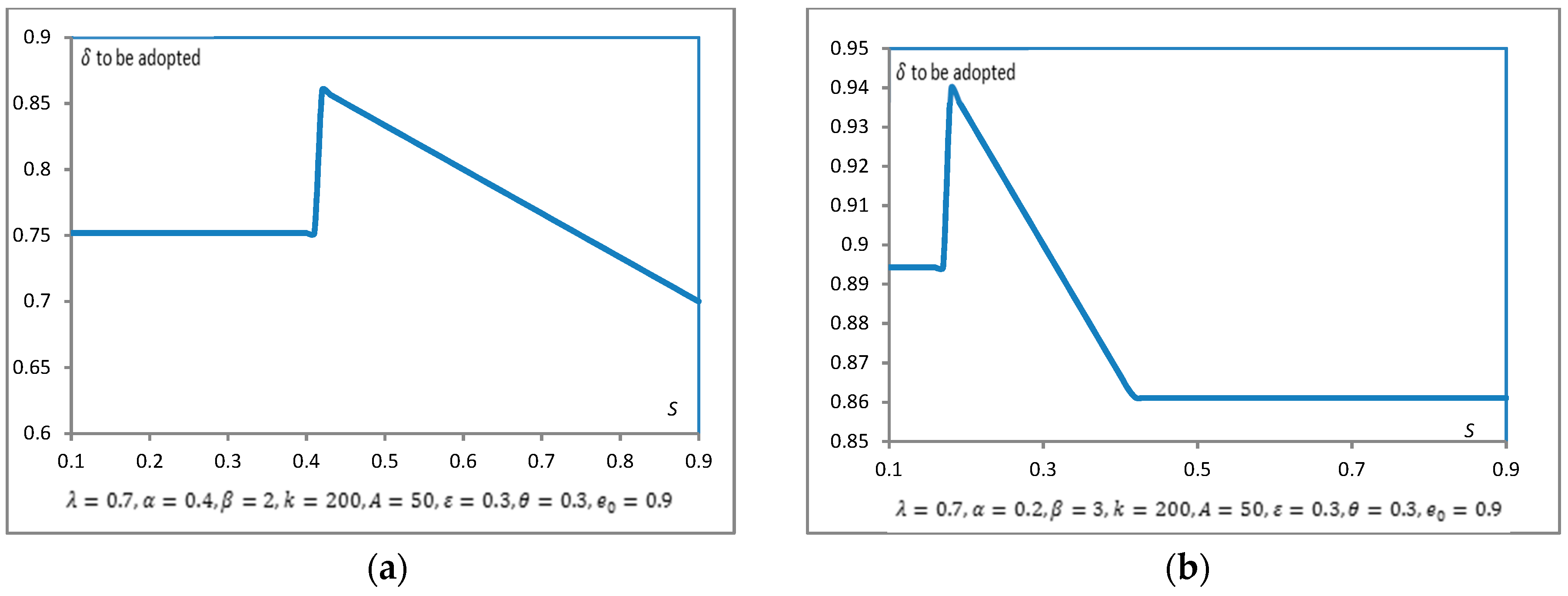
Proposition 4 and 5 can be further explained with the help of Figure 1 and Figure 2.

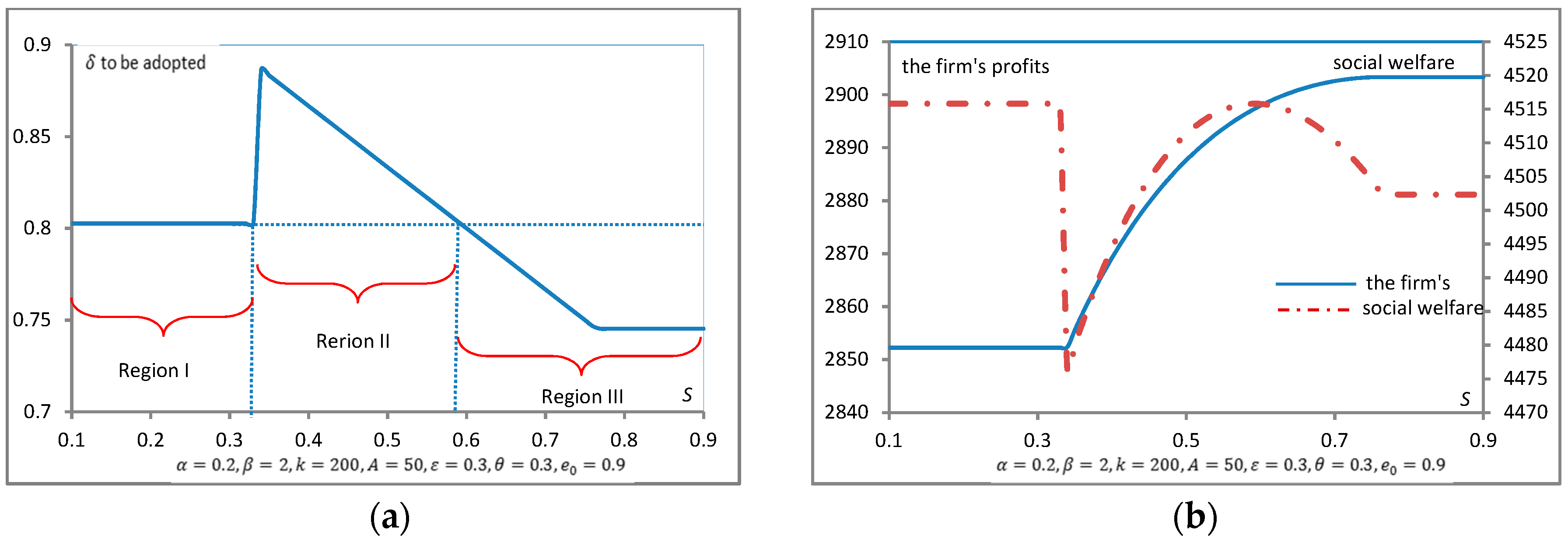
Figure 1 shows that when other parameters remain unchanged, the firm and the regulator will face three situations (identified by Region I, Region II and Region III in Figure 1 and Figure 2) along with the change of $S$. Region I indicates the case that the firm will not take the ETD incentive if $S$ is so strict that the benefits of tax deduction may not be sufficient to offset the higher cost for it. In Region II, the revenue increased by tax deduction for the firm can offset the additional investment to reach a higher $\delta$ which meets the ETD incentive threshold. However, for the regulator, the social welfare does not necessary increase when the firm switches from Region I to Region II with a cleaner technology, implying that to achieve a higher emission reduction level $\delta$ the whole society needs to pay the corresponding cost. In this case, although the firm needs more investment to achieve a higher green level, the government’s tax deduction and higher retail prices are enough to compensate for the costs since production does not react to the environmental tax, so the firm’s profits is increased. However, in the government profit function, investment in pollution reduction cannot be offset by the resulting reduction in pollution damage, resulting in a decline in social welfare. It is also showed that in Region II the highest profit of regulator is as much as that in Region I; however, the corresponding $\delta$ decreases to the same level as of that in Region I with the increase of $S$. Region III is the case where $S$ is too high to persuade the firm to switch to a higher $\delta$ than that in Region I. In other words, the firm can enjoy the benefits of tax deduction without increasing the level of emission reduction, implying that Region III should not be a favorable case for the regulator.

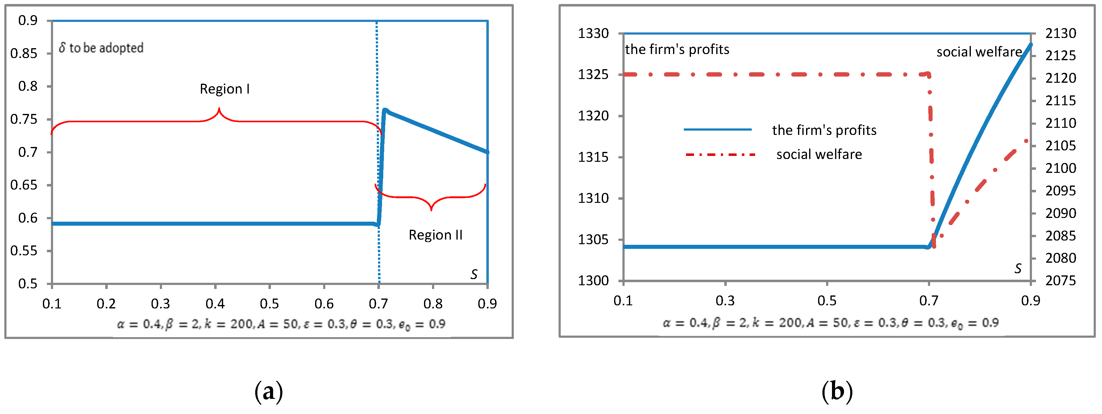
Specially, Figure 2 shows a scenario that the firm faces a more price-sensitive market ($\alpha =0.4$ compared to $\alpha =0.2$ in Figure 1), in which it is more difficult for regulator to convince the firm to choose the ETD option unless with a looser emission standard $S$. This is intuitive since a more price-sensitive market provides less room for the firm to invest in green technology to reduce pollution emissions.

4. Game with Decision Weights

4.1. Without ETD

In this section, the authors assumed the regulator assigns different decision weights to economic surplus and environmental damage. This is a reasonable assumption in reality as countries at different stages of development have different focuses on economy and environment. Some emerging economies like China may pay more attention to economic development at the initial stage, but now the regulator is increasingly concerned about environmental protection.

Based on this assumption, we denote $\lambda (0<\lambda <1)$ as the weight assigned to environmental objects and $1-\lambda$ to economic ones by the regulator. A higher $\lambda$ means the regulator has a higher degree of environmental concern/awareness. Then, the regulator’s profit would be given by:

$${\Pi }_r^{W\_B}=(1-\lambda )({{\displaystyle \int }}_0^{q}p(x,\delta )dx-qp(q,\delta )+{\Pi }_f)+\lambda (T-\epsilon {(q{e}_0(1-\delta ))}^2/2)$$

(12)

where ${\Pi }_f^B$ is given by (5) and $T\equiv qt{e}_0(1-\delta )$. ${\Pi }_r^{W\_B}$ in Equation (12) consists of two components, i.e., economic issue and environmental protection issue. Anticipating the firm’s reaction to the environmental policy, the regulator with a decision weight needs to solve the following optimization problem:

$$\underset{t}{\max }{\Pi }_r^{W\_B}=(1-\lambda )\left({{\displaystyle \int }}_0^{q}p(x,\delta )dx-qp(q,\delta )+{\Pi }_f\right)+\lambda (T-\epsilon {(q{e}_0(1-\delta ))}^2/2)$$

(13)

Let $\mathrm{L}\equiv \sqrt{{\lambda }^2{\beta }^2+4\lambda (1-\lambda )\epsilon k{e}_0{}^2}$, then we have the following propositions:

Proposition 6.

In case of $\frac{{\beta }^2}{2{\beta }^2+\epsilon k{e}_0{}^2}<\lambda <1$: (i) The regulator’s optimal $t^{*W\_B}$ and the firm’s corresponding ${\delta }^{*W\_B}$ are:

$$t^{*(W\_B)}=\frac{(3\lambda -2)\beta +L}{2(1-\lambda )e_0}$$

(14)

$${\delta }^{*W\_B}=1-\frac{8(1-\lambda )\alpha k}{(\lambda \beta +L)(A+\beta +\sqrt{H})}$$

(15)

In particular, $t^{*(W\_B)}=t^{*(B)}$ when $\lambda =0.5$.

(ii)The optimal $t^{*(W\_B)}$ increases with $\lambda$ and $\epsilon$, i.e., $\frac{d{t}^{*(W\_B)}}{d\lambda }>0$, $\frac{d{t}^{*(W\_B)}}{d\epsilon }>0$, and the optimal ${\delta }^{*W\_B}$ increases with $\lambda$, i.e., $\frac{d{\delta }^{*(W\_B)}}{d\lambda }>0$.

See Appendix D for the proof.

Besides, it is easy to check that $\frac{d{\delta }^{*(W\_B)}}{d\beta }>0$, $\frac{d{\delta }^{*(W\_B)}}{d{e}_0}>0$, $\frac{d{\delta }^{*(W\_B)}}{d\epsilon }>0$ and $\frac{d{\delta }^{*(W\_B)}}{d\alpha }<0$, and the proof is not mentioned here.

Proposition 7.

(i) In case of $\frac{2}{3}\le \lambda <1$, $\frac{d{t}^{*}}{d{e}_0}<0$, $\frac{d{t}^{*}}{d\beta }>0$. (ii) In case of $\frac{{\beta }^2}{2{\beta }^2+\epsilon k{e}_0{}^2}<\lambda <\frac{1}{2}$, $\frac{d{t}^{*}}{d{e}_0}>0$, $\frac{d{t}^{*}}{d\beta }<0$.

See Appendix E for the proof.

Since in this paper, the authors only considered tax policy ($t^{*(W\_B)}\ge 0$) regardless of the subsidy policy (denoted by the case of $t^{*(W\_B)}<0$), it can be seen from Proposition 6 that the regulator with an environmental concern weight can set a feasible tax rate only when his decision weight $\lambda$ is greater than $\frac{{\beta }^2}{2{\beta }^2+\epsilon k{e}_0{}^2}$. One can also infer from Proposition 6 that $t^{*(W\_B)}$ increases in $\lambda$. This conclusion is straightforward, because the more environmental concerns, the more the regulator tends to adopt higher tax levels. However, it should be noted that Proposition 7 presents two opposite situations. A regulator with high level of environmental concerns (denoted by the case of (i)) would be “merciful” to a dirtier firm (i.e., $\frac{d{t}^{*}}{d{e}_0}<0$) for knowing that the dirtier firm will pay more effort on pollution reduction (i.e., $\frac{d{\delta }^{*(W\_B)}}{d{e}_0}>0$), being more consistent with consumers’ arguments (i.e., $\frac{d{t}^{*}}{d\beta }>0$) for the fact that it left more room for the regulator to increase tax rate if consumers favor green products and are willing to pay extra costs for low-pollutant products; however, a regulator with low $\lambda$ (in the case of (ii)) opts for the opposite.

4.2. With ETD

Similar to Section 3, the regulator, who puts different decision weights on economic surplus and environmental damage, promises that if the firm’s per unit emissions $e_0(1-\delta )$ is below $\theta (0<\theta <1)$ percent of a given emission standard $S$, then the environmental tax can be reduced to $t^{*(W\_B)}(1-\theta )$. Considering this incentive, the firm will first examine whether his optimal reaction meets the requirements of (8) and will solve the following optimization problem:

$$\underset{q,\delta }{\max }{\Pi }_f^{W\_ETD}=q(p(q,\delta )-t^{*(W\_B)}(1-\theta )e_0(1-\delta ))-c(\delta ))$$

(16)

Similar to proposition 1, given an environmental tax $t^{*(W\_B)}(1-\theta )$, the optimal $\delta$ for the firm is:

$${\delta }^{*(W\_ETD)}=1-\frac{4\alpha k}{(\beta +t^{*(W\_B)}(1-\theta )e_0)(A+\beta +\sqrt{H})}$$

(17)

Proposition 8.

${\delta }^{*(W\_ETD)}$ will always be the firm’s reaction to the tax cuts if $\frac{8(1-\lambda )\alpha k{e}_0}{\theta (A+\beta +\sqrt{H})\left[(\lambda -3\theta \lambda +2\theta )\beta +(1-\theta )L\right]}<S<e_0$ holds.

Proof of proposition 8 follows directly by noting that ${\delta }^{*(W\_ETD)}<{\delta }^{*(W\_B)}$ and substituting (17) into (8) to fulfill the ETD threshold. Therefore, this proof is also not mentioned here.

However, if $S<\frac{8(1-\lambda )\alpha k{e}_0}{\theta (A+\beta +\sqrt{H})\left[(\lambda -3\theta \lambda +2\theta )\beta +(1-\theta )L\right]}$, it is implied that the firm must adopt a higher $\delta (\delta >{\delta }^{*(W\_ETD)})$ to meet the ETD policy threshold. Since the profit is decreasing with $\delta$ if $\delta >{\delta }^{*(W\_ETD)}$, the firm needs only to examine if the lower limit of $\delta$ in (8) is an acceptable solution.

Let ${\delta }^{\prime (W\_ETD)}=1-\frac{\theta S}{e_0}$, and by substituting ${\delta }^{\prime (W\_ETD)}$ together with $t^{*(W\_B)}$ and $q^{*(B)}$ into (16), we have:

$$\begin{gathered} {\Pi }_f^{\prime (W\_ETD)}=\frac{A+\beta +\sqrt{H}}{4\alpha }\left(\frac{3(A+\beta )-\sqrt{H}}{4}-\frac{\theta S((\lambda -3\theta \lambda +2\theta )\beta +(1-\theta )L)}{2(1-\lambda )e_0}\right) \\ +kln(\frac{\theta S}{e_0}) \end{gathered}$$

(18)

Proposition 9.

The regulator with a decision weight $\lambda$ on environmental damage may not be able to motivate the choice of ${\delta }^{\prime (W\_ETD)}$ through the ETD incentive policy unless $\mathsf{\Delta }{\Pi }_f{}^W= {\Pi }_f^{*(W\_ETD)}-{\Pi }_f^{*(W\_B)}\ge 0$ in case of $S<\frac{8(1-\lambda )\alpha k{e}_0}{\theta (A+\beta +\sqrt{H})\left[(\lambda -3\theta \lambda +2\theta )\beta +(1-\theta )L\right]}$.

Proof of proposition 9 is straightforward since the tax incentive makes no sense if $\mathsf{\Delta }{\Pi }_f{}^W= {\Pi }_f^{*(W\_ETD)}-{\Pi }_f^{*(W\_B)}<0$ for the firm.

Proposition 8 and 9 can be further explained with the help of Figure 3, Figure 4 and Figure 5.

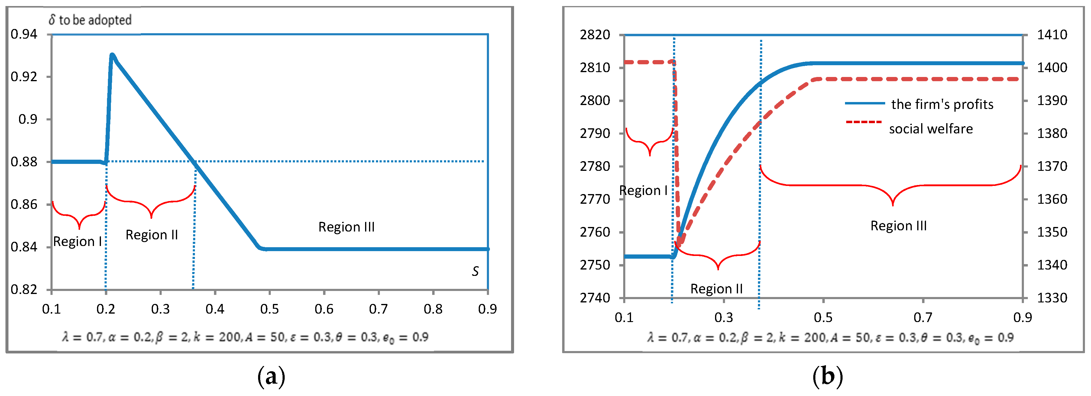
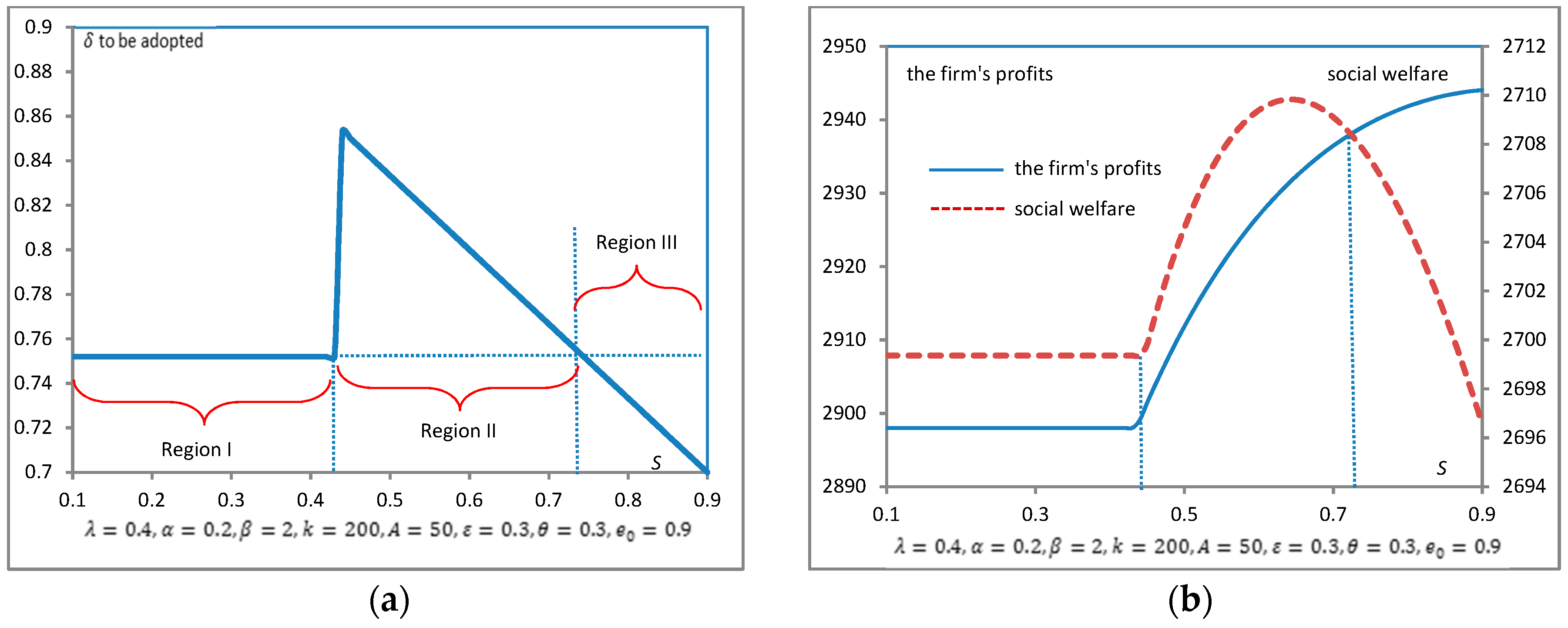
Compared with Figure 1a, in which case the decision weight of economic surplus and environmental damage is equal, Figure 3a and Figure 4a show that the firm will adopt a higher/lower emission reduction level when facing a regulator with a higher/lower degree of environmental concern ($\lambda =0.7$/$\lambda =0.4$). From Figure 3 and Figure 4, one could also notice that the regulator needs to exert a higher $S$ to induce the firm to switch to the ETD solution as $\lambda$ decrease. This is no surprise. When the regulator is not concerned about the environment, it will choose a lower environmental tax and consequently the ETD policy is unattractive to the firm since the tax deduction space has been reduced for a given $\theta$ and the firm is reluctant to invest money on green technology in exchange for tax reduction. From Figure 3 and Figure 4, It is also concluded that the firm’s profit and social welfare will both decrease as $\lambda$ increases. This can be interpreted mostly by our assumption of the green investment cost function, $c(\delta )$, implying that the firm’s profit margins will decrease sharply with the increase of $\delta$ which corresponds to a higher $\lambda$. However, Figure 4b shows that for the cases with moderate level of environmental concern and emission standard, the regulator can set an ETD incentive to motivate the choice of higher level of emission reduction and simultaneously increase social welfare.

Comparing Figure 5 with Figure 3, it would be deduced that the firm will be more reluctant to accept the ETD solution as the market becomes more price-sensitive (see Figure 3a with $\alpha =0.2$ and Figure 5a with $\alpha =0.4$). On the contrary, when the market’s environmental consciousness increases, it is easier for the regulator to guide the firm to adopt ETD solution (see Figure 3a with $\beta =2$ and Figure 5b with $\beta =3$). This is reasonable since a more price-sensitive market offers less room for the firm to finance green technology than a low-emission-sensitive market, and the firm cannot demand a higher price for his effort of emission improvement. Thus, the firm will not increase emission reduction level to reach the threshold of the tax incentive policy unless the emission standard is relaxed.

5. Discussion

In order to encourage the greener behavior of production firms through environmental tax deduction incentive, the authors investigated manipulation of Stackelberg game model between a firm and regulator. A look back at the existing literature reveals that the preceding researchers have found that: (i) the green technology level, environmental improvement coefficient and unit cost increase coefficient play important roles in the government environmental policy strategy and (ii) the firm’s reaction to an increase in taxes may be non-monotone while an initial increase in taxes may motivate a switch to a greener technology, and further tax increases may motivate a reverse switch (Krass et al. [14] and Bi et al. [22]). The current work partially corroborates with these two conclusions. However, it cannot be ignored that consumers’ environmental consciousness as well as regulator’s environmental concern are important factors in promoting enterprises’ green investment.

In a market with high environmental awareness, enterprises will adopt a higher level of green investment, while the government does not need to adopt a higher tax. Thus, the market driver can be most effective in any case.

In the current study, there indeed was a monotone relationship between the regulator’s tax and green investment level of the firm. However, the tax cannot be increased indefinitely, for which the optimal level is defined by other factors mainly including $\epsilon$, $k$, $\beta$ and $\lambda$. Nevertheless, this was not the focus of this study. This work’s emphasis was whether the regulator can further influence the green decision-making of the firm through an ETD policy.

The regulator’s environmental concern weight was another significant consideration in this work, which represents the regulator’s subjective tendency towards economic and environmental values, and thus determines the definition of social welfare. When the regulator adopts equal focuses on the economic and environmental aspects, some incentive policies to improve the green level of the firm do not seem to improve social welfare. However, if the regulator differentiates between economic and environmental welfare, it may find the best incentive policies to induce the firm’s green behavior as well as increase total social welfare.

The regulator tax policy will only affect the emission reduction level, but cannot influence the output of the firm. Based on the model of this research, the firm’s optimal production quantity mainly depend on three factors: $\alpha$, $\beta$ and $k$, and the result showed that the firm tends to produce less if consumers are sensitive to price, or emission reduction is difficult. However, if consumers have strong environmental awareness and are willing to pay extra costs for low-pollutant products, the firm will increase the output as well as the emission reduction level. As a result, improving consumers’ awareness of environmental protection is an effective way to promote green investment of firms. Although the government can guide enterprises to raise the level of emission reduction through increasing taxation, the optimal level of tax rate will be constrained by market and business operational factors.

6. Conclusions

The current paper investigated Stackelberg games between one profit-maximizing firm producing a particular product (followers), and a regulator, the leader that has the power to set the environmental tax, to induce green initiative by the firm. Two cases were addressed according to whether the regulator has a decision weight between economic and environmental profit or not. For each case, the researchers first examined the factors that affect the firm’s level of pollution reduction and the regulator’s tax rate in the equilibrium state. Then the impact of ETD option offered by the regulator on the firm’s green investment was discussed further. Through numerical analysis, different cases were investigated and the corresponding discussions were conducted to generate insight for decision-making bodies and involved stakeholders.

The analyses carried out here show that whether the firm accepts the regulator’s ETD incentive option depends on market and operational factors. The firm will be more reluctant to accept the ETD solution as the market becomes more price-sensitive. However, when the market’s environmental consciousness increases, it is easier for the regulator to guide the firm to adopt ETD solution. In any case, the firm will adopt ETD solution only if its gains exceed its cost. For the regulator, it is necessary to set an appropriate level of emission standards as too strict standards lead to ignoring the ETD incentive by the enterprise, and too loose standards may seem meaningless for motivation of the green initiative. The results also indicate that the regulator’s environmental concern is an important factor to induce the firm’s green behavior. The high level of environmental concern pushes the tax rate to a high level where the ETD option is more attractive to the firm. By contrast, when the regulator is not concerned about the environment, it will choose a lower environmental tax and consequently the ETD policy will be unattractive to the firm since the tax deduction space has been reduced and the firm is reluctant to invest money on green technology in exchange for tax reduction. However, even if the firm adopts a higher level of emission reduction solution, it does not necessarily mean that the whole social welfare will be raised.

In any case, it is worth noting that all these results should be explained in the context of the introduced model, which focuses on the impact of tax-only incentives on the firm’s efforts to reduce pollution emissions in a monopoly situation. In future work, the authors wish to discuss the situation of Cournot oligopoly. Other extensions can explicitly include uncertainty in demand, asymmetry in information, and the cost of technology. Furthermore, the presented stylized model here, does not take into account many of the implementation-related complexities, namely, how companies can accurately understand the environmental concerns of regulators, and the administrative costs of designing the best policy merit more meticulous investigation.