Article

Flow Analysis and Damage Assessment for Concrete Box Girder Based on Flow Characteristics

1
Faculty of Science and Engineering, Waseda University, Tokyo 169-8050, Japan
2
Graduate School of Engineering, Kyoto University, Kyoto 615-8540, Japan
3
Public Works Research Institute, Tsukuba 305-8516, Japan
*
Authors to whom correspondence should be addressed.
Sustainability 2019, 11(3), 710; https://doi.org/10.3390/su11030710
Submission received: 26 December 2018 / Revised: 21 January 2019 / Accepted: 21 January 2019 / Published: 29 January 2019

Abstract

:
For a system such as the concrete structure, flow can be the dynamic field to describe the motion, interactions, or both in dynamic or static (Eulerian description) states. Further, various kinds of flow propagate through it from the very start to the end of its lifecycle (Lagrangian description) accompanied by rains, winds, earthquakes, and so forth. Meanwhile, damage may occur inside the structure synchronously, developing from micro- to macro-scale damage, and eventually destroy the structure. This study was conducted to clarify the content of flow which has been implicitly used in the damage detection, and to propose a flow analysis framework based on the combination data space and the theory of dissipative structure theory specifically for nondestructive examination in structural damage detection, which can theoretically standardize the mechanism by which flow characteristics vary, the motion of the structure, or the swarm behavior of substructures in engineering. In this paper, a destructive experiment (static loading experiment) and a following nondestructive experiment (impact hammer experiment) were conducted. According to the experimental data analysis, the changing of flow characteristics shows high sensitivity and efficient precision to distinguish the damage exacerbations in a structure. According to different levels of interaction (intensity) with the structure, the information flow can be divided into two categories: Destructive flow and nondestructive flow. The method used in this research is named as a method of “flow analysis based on flow characteristics”, i.e., “FC-based flow analysis”.

1. Introduction

From some damage surveys [1,2,3] in Japan and the United States of America, bridges are deteriorated or damaged by material aging, overload, fatigue, temperature, corrosion, rust, and disasters such as earthquakes, hurricanes, and so forth. In addition to the natural factors, various kinds of damage may occur for the following reasons: (a) Nonconservative design, (b) severe service environment, and (c) improper construction or operation management maintenance. No matter whether the damage is caused by nonhuman factors or human factors, the damage usually initiates at a microscopic level, grows and extends to a macroscopic level, and eventually causes the collapse of a structure when the damage is not detected in time. The detection and evaluation of the potential damage and minimization of the probability of structural failures are keen issues for many countries in the world.
There are many damage detection methods. They can be majorly categorized into the destructive examination and nondestructive examination (NDE) [4]. NDE is a group of damage detection methods that do not affect or harm the test material, component, or system, such as ultrasonic testing (UT), radiographic testing (RT), infrared thermography (IT), and acoustic emission (AE), among others. In the laboratory experiment, the NDE is often conducted to test the damage after some static loading experiment (one kind of destructive experiments, which would cause damage to the structure). If we view the above methods from a general point, many of the NDE methods share a common concept to show the change of structural status: “dynamic field [5]” or otherwise named as “flow”. The dynamic field (flow) is a term defining a field with smooth uninterrupted movement or progress in physics, very commonly used in fluid mechanics nowadays, and also implicitly used in NDE methods; for example, the electromagnetic field in RT and the sound field in AE. Simultaneously, in the static loading experiment, there is a stress field [6] and crack-tip stress field [7] in the static stress–strain response.
According to Newton’s third law, in the research of damage detection, a global system consists of three parts: The target structure, the environment (referring to everything outside the target structure with a limit domain), and interactions (often described as one kind of flow). In the common sense, an equilibrium state is the state in which the system state variables remain unchanged, as originated from thermodynamics and applied in various departments. The equilibrium state is also commonly studied in dissipative structure theory [8] (one special kind of system theory for but not only restricted to nonequilibrium thermodynamics describing the system “far from equilibrium state”) and general system theory (the general system theory often concerns the system near “equilibrium state”), and exists in the water flow on dams and bridges, wind on buildings, rain on steel plants, and radiation in nuclear reactors, and so on; even for vibration in an ordinary concrete beam-like structure. For these systems, which can realize their new balance in self-organization [9] (a system can continuously reduce its entropy and improve its order by exchanging substance, energy, and information with the outside world), if the structures are nonlinear and nonstationary, there may be many equilibrium shifts (the process from one equilibrium to another, i.e., “the process from an equilibrium state to a nonequilibrium state, and then to another equilibrium state”, or “from an equilibrium state to another equilibrium state directly in a short time”). In the global systems, the state variables describing the flow characteristics in multiple equilibrium shifts may dynamically fluctuate. For the reason that it is almost impossible to describe the evolutions of equilibrium and nonequilibrium states chemically and physically for these highly complex structures [10], it is difficult to obtain an analytical solution for the problems within the dynamic field (for example, turbulent flow). Then, to understand the flow in terms of structural damage detection, the black-box methods involving only inputs and outputs or grey-box methods involving inputs, outputs, and certain structural features could be used. Moreover, in solid mechanics, the flow can be described as vibration by the Eulerian description, which concerns the change of the whole dynamic field and can be modeled as a function of time; also, the flow can be described as a wave by the Lagrangian description, which concerns the difference between one place and another when the wave is propagating and can be modeled as a function of space. Though time is concerned in the Lagrangian description, the main issue we are concerned with is more about the space.
In recent years, to identify the potential damage in civil structures, the information model of the structure [11] for health monitoring concerns many kinds of structural characteristics as damage indicators, including flexibility and stiffness [12], frequency [13], damping ratio change [14], and mode shape [15], among others, in a variety of works through modal analysis, hazard analysis [16], and so forth. However, for comprehensively understanding the structural system in decision-making, more attention should be paid to the global system’s characteristics rather than solely to the structure characteristics, in acknowledging that all structures are more or less interacting with their environment. Therefore, the characteristics of the structural environment [17,18], as well as kinds of characteristics to describe the flow (flow characteristics), should be considered.
In this research, two kinds of flow are defined and classified in this research: Physical flow and information flow. Concerning the information flow, it has four classes of basic characteristics describing the spread of flow, the channel for flow, the flow amount in the channel, and the expansion of flow in the system. When the structure has damage, the equilibrium of swarm behavior [19] of the flow may immediately be broken and its characteristics changed at the same time. By analyzing these changing but distinguishable characteristics (such as via AE [20] and local wavenumber technique [21]), it is possible to evaluate whether the structure is damaged or not. Further, measuring data used in flow analysis can be directly inherited from general static and dynamic damage detection experiments. In this paper, an offline case of global damage evaluation for a structure (girder with artificial damage) is discussed in flow analysis by conducting a static experiment (static loading experiment and tendon-cut) and dynamic experiment (impact hammer experiment) to simulate the accelerated destruction and nondestructive examination for flow analysis to evaluate and diagnose the existing structures.
The paper is organized as follows: Following this introduction, the basic concept of the present FC-based method is given in Section 2. A laboratory experiment is conducted on two nearly full-scaled box girders to test the present method and its details are given in Section 3. In Section 4, experiment results are presented and discussed, including quantitative study, qualitative study, comparative analysis, error analysis, and possible applications. Finally, several concluding remarks and future works are summarized.

2. Basic Concepts of Flow Analysis

2.1. Definition and Classification of Flow

Flow is often referred to via simulating the phenomena which are similar to the motion of fluid [22] with a continuous tendency of points in time or space. From the perspective of mathematics, flow can be described as the dynamic field as a set of changes over time or space [23], i.e., flow is described as a group action of the real number on a set; for instance, a vector flow is determined by a vector field. A flow can be modeled as the function of time or space (t) as a group action of the additive real numbers on X [24]. More explicitly, a flow is a mapping of φ [25] in time or space t using the iterated function [26]:
φ ( t ) : X × X
The mathematical definition of flow is used widely in computational fluid mechanics and may be mainly used in the experimental data processing later.
In engineering, according to the observation of flow, a flow system can be divided into two categories: Incoming flow and outgoing flow. Since the flow is described as the function of the time or space, the flow in the previous space (sa) or previous time (ta) is the incoming flow (or referred to the input of flow and denoted as flowin), and the flow in the later space (sb = sa + s) or later time (tb = ta + t) is the outgoing flow (or referred to the output of flow and denoted as flowout). Sometimes a third category is considered: The cycling flow between incoming and outgoing flow within s or during t.
In our classification, there are two kinds of flow in mechanical engineering. The first kind is the flow whose carrier or intermedium moves along with it, such as the water flow in the river (hydromechanics); the second kind is the flow whose carrier or intermedium does not move along with it, only using the dynamic field of some information (such as “force, energy, momentum”, etc.) to describe the integral motion of some kind of space (with the function of time) in the Eulerian description, or the information field describing the motion passing through the space in the Lagrangian description (in mechanics, it means the transferring of interaction between structure and environment, or among substructures, from one point to another, represented as the function of space). In this paper, we name the first kind of flow as the physical flow and the second kind as the information flow (the flow describing the physical information of the system or the structure). In the following chapters, the information flow will be mainly discussed, and both the Eulerian description and Lagrangian description will be used when conducting the experimental analysis. Further, there are some other methods to classify the information flow, such as destructive flow or nondestructive flow, according to the influence on the structure; the information flow can be of either scalar, vector, or tensor nature.
Furthermore, for a measurement of a system, there are three kinds of views: microscopic, mesoscopic, and macroscopic [27]; so, in deeply understanding these, the research of flow can have three corresponding views:
  • In the microscopic view, it mainly focuses on the phonon (a phonon is a quantum mechanical description of an elementary vibrational motion in which a lattice of atoms or molecules uniformly oscillates at a single frequency) and the formation mechanism of flow (here, wave and flow have the same meaning).
  • In the mesoscopic view, it mainly concentrates on the evolution mechanism of basic flow, and how the basic flow (wave) joins to a swarm (here, the flow is treated as the swarm behavior of simple harmonic waves).
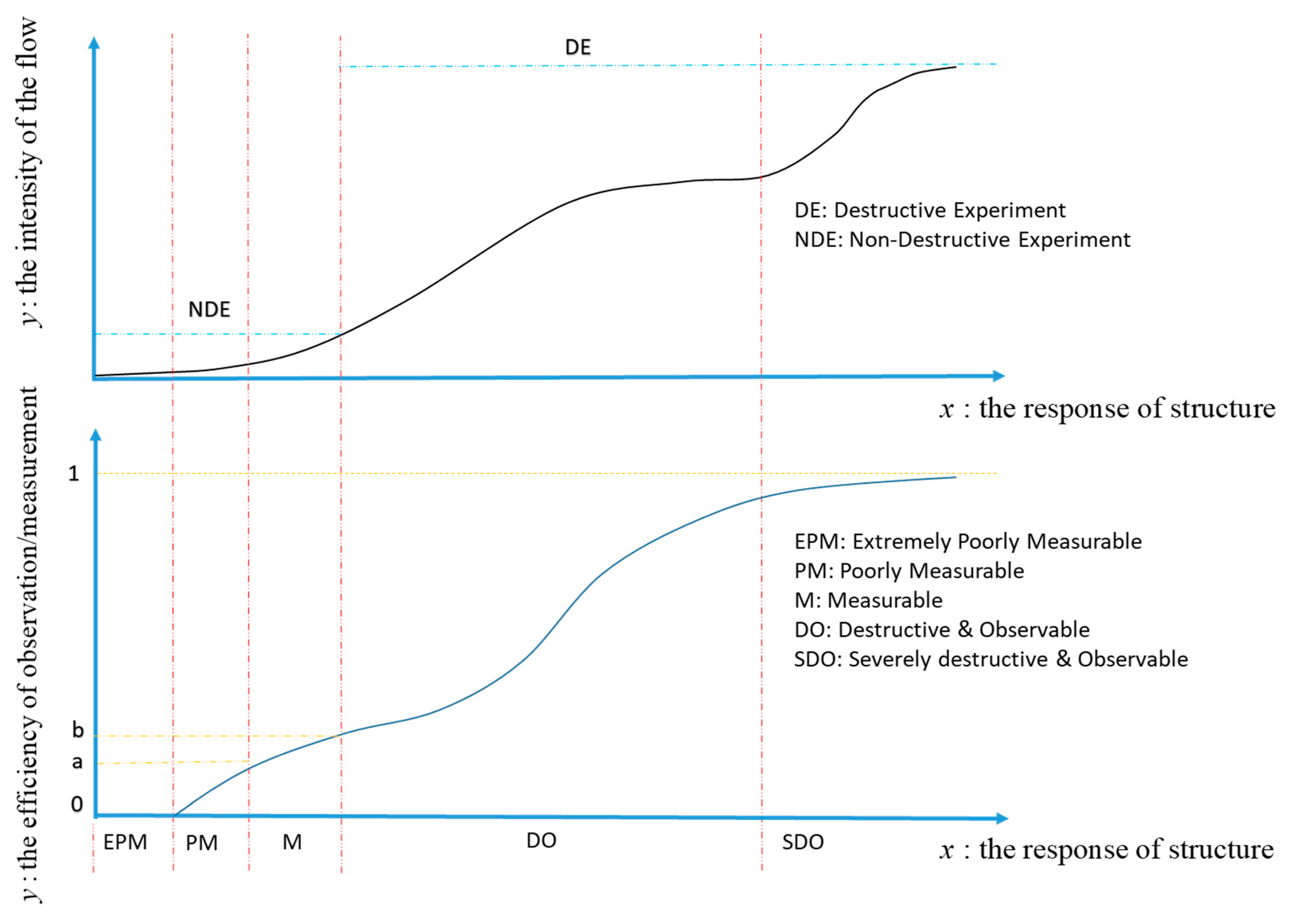
  • In the macroscopic view, the research is mainly for statistical mechanism and pattern recognition for the flow (usually, the flow is of turbulence, which is hard to describe using the analytical wave functions).
In this paper, the research aspects for the evaluation of a global system can be about structure, environment, and flow. For a specific environment in the measurement, suppose the data in any survey (recorded as time series, etc.) contain the information (i.e., some characteristics; according to the definition proposed by Wiener [28], information is a set of marks of a thing’s attributes) of the structure, environment, and flow simultaneously, more or less. This paper is trying to propose a new kind of damage analysis within a unified concept of flow.
In some sense, the interaction between environment and structure can be treated as the interactions between structure and flow, as well as between flow and the environment; the interactions among substructures can be converted as the interaction between substructures and flow. Analogous to the wave–particle duality [29] in physics, where the wave and particle are coexisting integrally, structure and flow are coexisting too, despite the description that particles show the system’s framework updating and the description that waves may reveal the system dynamically changing as well. Further, in some cases of statistical mechanics, it is more probable to know the behavior of the swarm rather than that of any individual; the statistical grouping parameters [30] of the motion of the waves can also be described as flow to show the trend of motion shown as the Lattice Boltzmann method (LBM) simulation in Figure A1 (Appendix A). To study the flow in the structure, in dynamics, flow analysis is to investigate the swarm behavior of the waves or vibrations (here, flow is equivalent to the swarm of waves in the structure from the view of space. Further, flow is equivalent to the swarm of vibrations in the structure from the view of time. Using different measuring equipment, the recorded data may be a time series of displacement, acceleration, velocity, etc.). In statics, flow analysis is used to investigate the field of force (here, flow is equivalent to a varying force field) or field of displacement (here, flow is equivalent to a varying displacement field), etc. However, in traditional structural mechanics for engineering, the structure itself (the particle perspective) is more likely to be concerned, such as for some structural characteristics in modal analysis, and the perspective of flow is often selectively ignored, and it is obviously insufficient. Moreover, if we consider the problem in damage analysis in the view of system, the structure and its environment are interacting (described by a dynamic field, i.e., flow) with each other continuously.

2.2. Flow Characteristics-Based (FC-based) Method

We often define the system Φ as a black box in many cases of damage detection. In the Eulerian description, for a field Θ existing in Φ and bounded by Φ, its status is denoted as φ ( t , Θ t 0 ) : A status of field depending on the time (t) and the initial condition Θ = Θ t 0   [31]. If φ ( t , Θ t 0 ) is a loop function (or its differential equals 0), the field may have a dynamic equilibrium corresponding to time. The interaction can described by field x, where x { μ , μ ˙ , μ ¨ , m μ ˙ , m μ ¨ , 1 / 2 m μ ˙ 2 } , in which μ is the displacement and m is the mass, and its status is   φ ( t , Θ t 0 ) ; this description of flow can be named as x-flow. Usually, the function of φ ( t , x t 0 ) is dependent on the nature of Φ. Further, the flow can be described in the Lagrangian description as the propagation in the system Φ; its change can originate from the Reynolds transport theorem as ψ ( s , Θ s 0 ) [32], which gives the flow’s propagation at point s and initial condition of Θ = Θ s 0 . If ψ ( s , Θ s 0 ) is near a constant in Φ, the medium of flow Φ is approximately homogeneous. In hydraulics, laminar flow is one such example. For a characteristic x to describe the field, its status is ψ ( s , x s 0 ) .
Combining two description methods, the input of the flow is defined as the initial condition   Θ t 0 , and output as the state of the flow Θ s t , where st is the point s in space at the point t in time.
In summary, the output of flow in time and space is influenced by the input ( Θ t 0   or Θ s 0 ) and intermedia (Φ). In the mechanical structure, the very simple but important example is the wave and vibration. The wave is the motion transmission in space from one point to another, and the vibration is a field varying in time from one moment to another. In Section 2.1, the flow in a vibrating structure is defined as the swarm of waves, as from the view of the Lagrangian description. In order to be closer to the concept of water flow in hydraulics, we will mainly continue using the Lagrangian description, but with some changes to meet our need to have a simple understanding of the vibration test data. Here are two assumptions:
  • Suppose for a system Φ, Φ is the surface of this system. The system can store or release the same flow as the flow of input, and the flow stored or released by Φ is flowΦ.
    flow in = flow Φ + flow out
  • h(t) and h(t,Φ) represent the input and output, respectively, and we record the input and output in the same period t , the effective input period [ t a 1 , t b 1 ] , and output period [ t a 2 , t b 2 ] :
    h ( t ) = t a 1 t b 1 ( Φ | j 1 | d ( Φ ) ) d t ; h ( t , Φ ) = t a 2 t b 2 ( Φ | j 2 | d ( Φ ) ) d t
    in which j1 and j2 are the flux at the differential surface d ( Φ ) of the input and output, respectively, which is the function of time and system, j = g ( t , Φ ) . For the same flow, the input lasts for ( t b 1 , t a 1 )   and the output lasts for ( t b 2 , t a 2 ) . Then, to calculate the flowΦ, here is its function, f (Φ):
    f ( Φ ) = h ( t , Φ ) h ( t )
Another comprehensive theoretical research work can be found on energy conservation law [33]. The change of the flow shows responses in the change of the system (intermedium) in turn. An infrastructure or any other open system [34] will have interaction with its environment in that the flow between the system and its environment is always changing but is often stable in statics by surveying data of times of measurement; the same relationships are seen among the interactions of different subsystems. However, in engineering applications, the process of flow propagation from the location of input to the location of output may often be impossible to investigate in practice, especially the sum of outputs in a structure with a complex shape of surface.
Then, the flow characteristics are suggested to approximately indicate the change of flow. For a specific system, if the flow can stably go through the system, these characteristics may not change as well. Furthermore, for the damage detection and identification, the FC-based method pays close attention to the damage spreading (e.g., the growth of cracks), structural integrity (e.g., structural disintegration process), signal propagation in the system (e.g., the change of frequency), migration of equilibrium between load effects, and resistance, etc. Kinds of structural parameters are also used to describe the change of flow in confined time or space [35], such as the changing of energy propagation or force distribution in a system. Sometimes in dynamics, flow can also be treated as the integration of waves. However, usually, in order to distinguish itself from other methods, the FC-based method mainly concerns the change of flow characteristics to evaluate the health of flow itself or indirectly diagnose the health condition of the system. According to the description of a general system, some basic concepts such as the development of interactions between a system and its environment, or among subsystems, frameworks, components or elements, boundaries, etc., will be considered [36,37]. Four classes of basic flow characteristics are proposed correspondingly to these four concepts of a general system:
Class 1:
Spread of flow: The characteristics to describe the spread of flow in the system, such as acceleration, speed, travel or propagation time, displacement, etc.
Class 2:
Channel for flow: The characteristics to describe the channel that the flow goes through. It is about the distribution of flow in the system and the route of flow in the system, such as its topology, hierarchy, fractal dimension, cross-sectional area, etc.
Class 3:
Flow amount in the channel of flow: The characteristics to describe the amount of flow, such as mass, quantity, intensity, strength, etc.
Class 4:
Expansion of flow in the flow system: The characteristics to describe the expansion of flow in a specific system or systems with or without clear boundaries, such as lifetime and propagation region (depth, width, or boundary).
Every flow has these four classes of characteristics, and according to some characteristics, flow can be classified conversely.
Of all criteria of differentiating kinds of flows, the intensity of flow is one simple standard. In a thought experiment, suppose there is an instrument with a certain accuracy which can be used to measure the response of the structure in any situation and there is a man who will observe the response of the structure with his naked eye. As the Figure 1 shows, when the flow’s intensity increases, the structural response, which directly influences the observability and measurability, may be more easily observed and measured such that the efficiency of observation and measurement will increase, and the damage detection will also transition from a nondestructive experiment (which is similar to the nondestructive examination) to a destructive experiment (which is usually different from the destructive examination, such as the chemical analysis of a core sample).
When the intensity grows from small to large, the response of the structure can be divided into EPM (extremely poorly measurable), PM (poorly measurable), M (measurable), DO (destructive and observable), and SDO (severely destructive and observable). Moreover, flow is not only the cause of structural damage which interacts with the structure and influences the state of structure, but also is influenced by the structural damage. As a result, once the state of the structure changes, the flow may change immediately.
In the general understanding of Figure 1, for the DO and SDO, the response of the structure to the flow can be linear and even at an exponential level; in such cases, the efficiency of measurement and observation can be much higher and even near 1, such that people can directly notice the state change of the structure with minimal error in observation. While for the M and the PM, the response of structure is nonlinear, even index or logarithmic, which cannot be observed by the naked eye directly, and how to define the exact value or the value of boundary efficiency a, b depends on the specific measurement or different standard.
For the EPM, the efficiency often equals 0, and the general tools of measurement are useless. In fact, the increased accuracy, recognition, and sensitivity of the experimental equipment could further expand the range of the observable and measurable. Further, for the cases of the DO and the SDO, the change of the response can be directly measured. Moreover, of all kinds, for the case of the PM, the corresponding flow is much more important in that it can help to detect more changes of the structure. So, in the design of the experiment, there are two aspects to be specially considered.
On the one hand, for the reason of the interaction between some flows and structures, the structural damage should be clearly observed along with the intensity of flow increasing. On the other hand, some flows can be used to detect the change or the damage of the structure independently. In the following chapters, for the static loading experiment (of the DO and the SDO, which bring great damage to the structure), the response of the structure is displacement, and for the impact hammer experiment, or named as the vibration experiment or impact tests (of the PM, which does not bring new damage or only brings small damage to the structure), the response of the structure is acceleration.

3. Experiment and Analysis of Artificial Damage

3.1. Introduction to the Experimental Design and Process

Since the experiment in this research is to check the structural healthy condition (with artificial damage), the structural artificial damage should continue to increase while the residual capacity of resistance should continue to decrease. In general, static research, the stress–strain curve shows the response of the structure to the flow, in that the change of the displacement field illustrates the intrinsic variation of the structural resistance. Further, in the modal analysis for dynamics, with high probability, one lower-order natural frequency of the structure will approximately decrease within a limited magnitude [38], while the damping ratio of this frequency will usually approximately increase [39] if there are some continuous damages. The structural characteristics for comparison in these studies include displacement, frequency, damping ratio, and so on. The whole experiment contains two subexperiments: The static loading experiment and the impact hammer experiment. The following is a brief introduction to the experimental preparation, experimental progress, and experimental numerical representation.
First, the preparation for the experiment is discussed. The survey paid attention to the common and same data used in other research, such as the loading (kN) and displacement (mm) in the static loading experiment, and acceleration (m/s2) in time series in the impact hammer experiment. Further, it was an indoor experiment so that the temperature and humidity would be in a controllable range that did not influence the process of the experiment.
Second, the experiment tested 3 nearly full-scale prestressed reinforced concrete open-section box girders (in short, box girder), named box girder 1, box girder 2, and box girder 3, by adding artificial damage. In this paper, only box girder 2 and box girder 3 (of the same design) were concerned especially for flow analysis. Both girders were in the same design, as shown by Figure 2 and Table 1: 8500 mm long, 2300 mm wide, and 1000 mm high. Further, there were 4 SDP-200 displacement meters, 8 SDP-100 displacement meters, and 10 ONOSOKKI-NP-2120 acceleration sensors set in different locations as shown in Figure 2, and the type of impact hammer used was the Brüel and Kjær type 8208.
The concentrated force was loaded at the middle of the structure. The impact hammer experiment was conducted in 9 stages (Table 2, Figure 3). Meanwhile, in every stage, the impact hammer experiment was after every experiment of static loading or tendon cut. A stage here means a series of tests of static loading experiment (or one time of tendon cut), impact hammer experiment, or both of them, and there is a series of increasing loading from 0 to the greatest loading in this stage, which then decreases to 0 with a series of loading steps, or one whole process of tendon cut. A step means a step change in force (maintained for a period of time). Every step of loading or tendon cut takes less than 15 min or 1 min, respectively.
The tendon cuts (in Figure 2) were conducted at stage 3 and stage 6, and the recovery after tendon cuts was at stage 4 and stage 7 for both box girder 2 and 3; for the tendon cuts of box girder 2, only 6 tendons were cut in total in the same side (the first time C1, C2, and C3; the second time C4, C5, and C6), while for the tendon cut of box girder 3, 12 tendons of both sides were cut; in the first time, they were C1, C2, and C3 in one side and C1, C2, and C3 in the other side; the second time they were C4, C5, and C6 in one side and C4, C5, and C6 in the other side.
Corresponding to the experiment, there are two kinds of damage: The damage caused by static loading and the damage caused by tendon cut. The crack development (Figure 4, the crack development in box girder 2) can be used to picture the damage development in the static loading. Since the damage happens inside the structure, we can only know that there is damage caused by the tendon cut but cannot observe it directly with the naked eye. However, we know that the damage is developing in the structure from stage 1 to 11 (or from steps 1 to 995 for box girder 2, and from steps 1 to 1150 for box girder 3).
Suppose the initial state of the structure is the healthy state (whose damage is 0), which means there is no damage, and the last state of the structure is a total failure (whose damage is 1), which means the system cannot satisfy its designed function. There is no need for us to know how much the damage is, and we just need to illustrate the increasing damage (from 0 to 1). If an indicator of damage can clearly indicate the damage development, it is qualified to be analyzed for the damage.
In this experiment, the acceleration sensors were located beneath the structure, while the same number of the hit points were designed further up the structure, directly above the corresponding sensors shown in Figure 5 (A1–A10).
Third, experimental numerical representation is discussed. There are 4 kinds of flow characteristics in data analysis.
(1) Intensity of distribution (IoD) in displacement flow (Figure 6): It means the displacement distribution in different locations for one step; in the analysis of the actual practical use, the reference step can be the step where the IoD corresponds to the load of 1/50–1/10 the design load.
Figure 7a shows the acceleration responses recorded by 10 acceleration sensors (corresponding to A1–A10). In the impact hammer experiment, there are another 3 kinds of characteristics for the acceleration flow shown in Figure 7b.
(2) Max-peak-time is from the first class of flow characteristics, i.e., spread of flow. In the acceleration time series, max-peak-time means the arrival time of “flood” (the max absolute value of amplitude in time series), starting from the time from the moment of the hit (contact between hammer and structure) to the moment of “flood”.
(3) Max-peak belongs to the third class of flow characteristics, i.e., flow amount in the channel of flow. The max value is the max peak of the amplitude (the max absolute value of amplitude) of the time series. It means the intensity of “flood”.
(4) Lifetime is classified in the fourth class of flow characteristics, i.e., expansion of flow in the flow system. The lifetime can be defined as the time from the moment of a hit to the moment of flow disappearance (the time from the moment when it is the end of the white noise to the moment when the flow vanishes and the new white noise begins again).
To investigate the whole system, we would take these data into a combined data space [40].
There, at every hit point, the impact hammer experiment would be repeated for many times. After many hits, a time distribution is found for those characteristics. Then, it is necessary to organize the data structure appropriately. In the following introduction, there are two kinds of matrices selected: The difference matrix for displacement flow and the combination matrix for acceleration flow.
On the one side, in the displacement flow, the static loading location is fixed at the right middle of the girder. There are 8 displacement meters of SDP-100, i.e., D2_UF, D2_UB, D2_LF, D2_LB, D5_UF, D5_UB, D5_LF, and D5_LB, located in different places. The record for meters is s = [s1, s2, s3,…, s8]. Then, a difference matrix is used to show the difference of displacement between every two meters. If the health condition of the structure is the same, the difference of displacement in the same situation (loading) may be the same, at least in a statistical sense. Then, the difference matrix is designed as:
s = [ s 1 , 1 s 1 , 2 s 1 , 3 s 1 , j s 1 , 8 s 2 , 1 s 2 , 2 s 2 , 3 s 2 , j s 2 , 8 s 3 , 1 s 3 , 2 s 3 , 3 s 3 , j s 3 , 8 s i , 1 s i , 2 s i , 3 s i , j s i , 8 s 8 , 1 s 8 , 2 s 8 , 3 s 8 , j s 8 , 8 ]
where si,j = sj,i means the absolute value of difference between displacements detected by the i - th and j-th meter (si,j=|si-sj|); i,j = 1,2,3,…,8. When si,j = 0, i = j.
On the other side, to evaluate the change of acceleration flow in different health conditions of the structure, the reasonable combination matrices for the flow characteristics should circumspectly involve the information of the locations of hit points and locations of sensors to logically show the change of the flow at the surface of the structure. (1) For the same health condition of the structure with a specific location of input (hit point), the record of sensors in different locations should be statistically the same; (2) for the same health condition of the structure with different locations of input (hit point), the record of sensor in the same location should be statistically the same as well. Then, the characteristic’s combination matrix contains both situations together, showing whether the structure is in the stabilization of the health condition or not. In our research, every expectation of max peak, max peak time, or lifetime (single value xi,j) are used to build every combination matrix. The impact hammer would strike on the structure from hit point 1 to 10, and for every hit, there are 10 sensors (j = 1,2,3,…,10) recording the data, and after 10 hits (I = 1,2,3,…,10) there are two time matrices: The max peak time (t) or lifetime (T) in the form of combination matrices.
t = [ t 1 , 1 t 1 , 2 t 1 , 3 t 1 , j t 1 , 10 t 2 , 1 t 2 , 2 t 2 , 3 t 2 , j t 2 , 10 t 3 , 1 t 3 , 2 t 3 , 3 t 3 , j t 3 , 10 t i , 1 t i , 2 t i , 3 t i , j t i , 10 t 10 , 1 t 10 , 2 t 10 , 3 t 10 , j t 10 , 10 ] & T = [ T 1 , 1 T 1 , 2 T 1 , 3 T 1 , j T 1 , 10 T 2 , 1 T 2 , 2 T 2 , 3 T 2 , j T 2 , 10 T 3 , 1 T 3 , 2 T 3 , 3 T 3 , j T 3 , 10 T i , 1 T i , 2 T i , 3 T i , j T i , 10 T 10 , 1 T 10 , 2 T 10 , 3 T 10 , j T 10 , 10 ]
where ti,j and Ti,j are the mean max-peak-time and lifetime of the i-th hit and j-th sensor, respectively. Meanwhile, the max-peak combination matrix is:
m = [ m 1 , 1 m 1 , 2 m 1 , 3 m 1 , j m 1 , 10 m 2 , 1 m 2 , 2 m 2 , 3 m 2 , j m 2 , 10 m 3 , 1 m 3 , 2 m 3 , 3 m 3 , j m 3 , 10 m i , 1 m i , 2 m i , 3 m i , j m i , 10 m 10 , 1 m 10 , 2 m 10 , 3 m 10 , j m 10 , 10 ]
where mi,j means the max peak of the i-th hit and j-th sensor.
Further, there are two kinds of data to indicate the change of the matrix in the acceleration matrix, value (such as the t, T, and m), and order. Each row of every matrix [xi,1, xi,1, xi,3,…, xi,10] means that in the i - th hit, all 10 sensors’ detection values get the ID of the sensor with the value from the maximum to the minimum or from the minimum to the maximum (this case will be used in this paper), or according to the specific requirement of the data processing. Here is an example:
n = [ n 1 , 1 n 1 , 2 n 1 , 3 n 1 , j n 1 , 10 n 2 , 1 n 2 , 2 n 2 , 3 n 2 , j n 2 , 10 n 3 , 1 n 3 , 2 n 3 , 3 n 3 , j n 3 , 10 n i , 1 n i , 2 n i , 3 n i , j n i , 10 n 10 , 1 n 10 , 2 n 10 , 3 n 10 , j n 10 , 10 ]
where ni,j means the order of max peak time of the i-th hit and j-th sensor. The example above shows the combination matrix of the order of max peak time, which means the sensors detect the signal one by one from the minimum value to maximum value.

3.2. Experimental Data Analysis

There are matrices of characteristic values or orders, such as s, t, T, m, and n in the research, for a general matrix M:
M = [ x 1 , 1 x 1 , 2 x 1 , 3 x 1 , j x 1 , a x 2 , 1 x 2 , 2 x 2 , 3 x 2 , j x 2 , a x 3 , 1 x 3 , 2 x 3 , 3 x 3 , j x 3 , a x i , 1 x i , 2 x i , 3 x i , j x i , a x b , 1 x b , 2 x b , 3 x b , j x b , a ] , { i = 1 , 2 , 3 , , a j = 1 , 2 , 3 , , b
where xi,j means the value at location (i, j); in our case, a = b.
To evaluate the data obtained in the experiment, there are six variables chosen to describe every matrix.
Note: The initial stage or reference is often selected as the first stage. Any two matrices describing the initial state (reference) and the state considered (test) are named Minitial and Mconsidered, respectively.
  • Determinant of the status matrix (if it is a square matrix)
    Determinant can be treated as the scaling factor of the transformation from a status matrix.
    For a column (n), row (n) matrix, its determinant can be defined by the Leibniz formula or the Laplace formula. Here in this paper, we use the Leibniz formula [41]:
    det ( M ) = δ S n sgn ( δ ) i = 1 n a i , δ i
    Here, all permutations δ are calculated as a summation of the set {1,2,3,…,n}.
  • Norm of the status matrix; the matrix norm extends the notion from vector norm to the matrix. For a matrix, when it meets these conditions, it can have the matrix norm:
    { | M | 0 ; every   matrix   belongs   to   ( R m × n )   vector   space | M | = 0 ;   if   and   only   if   M = 0 | α M | = | α | | M | ; every   α   is   in   ( R 1 × 1 )   vector   space   | M 1 + M 2 | | M 1 | + | M 2 | ;
    The calculation of status matrix norm is thus | M | = sup { | M x | ,   x ( R n × 1 ) ,   | x | = 1 } .
    In this research, we use the 2-order norm (Euclidean norm):
    | M | 2 = λ max ( M * M )   ; where M* is the conjugate transpose of M.
  • Max eigen or spectral radius of the status matrix, spectral radius: SR(M) = max(|λi|).
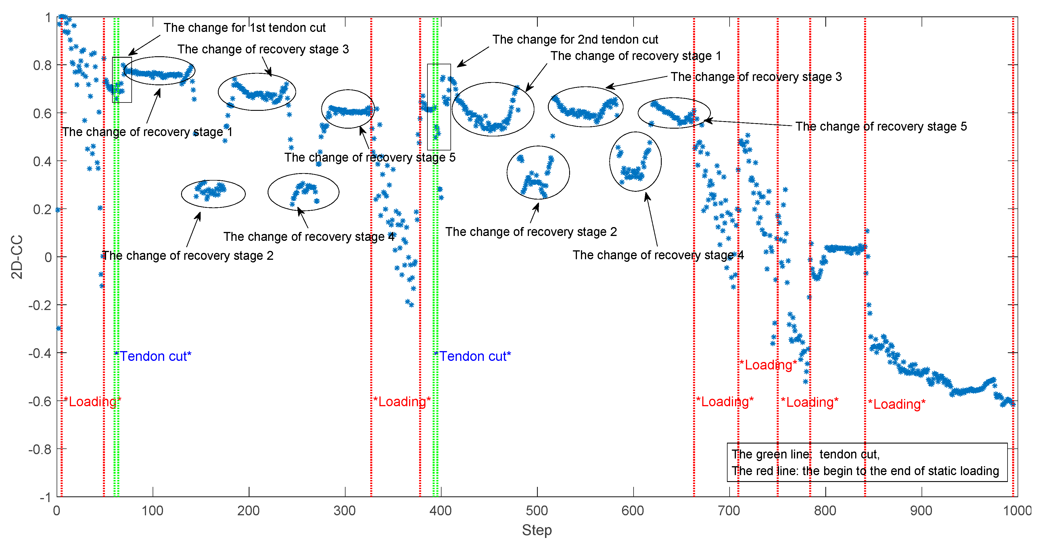
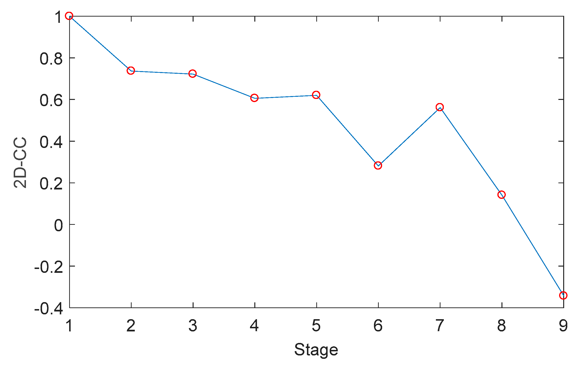
  • 2D correlation coefficient (2D-CC) between every considered status matrix and initial status matrix.
    The 2D-CC is usually used to distinguish the status matrix change between the initial state (reference) and the state considered (test) in this research. The definition of this technology is as follows:
    C = ( M initial T M ¯ initial T ) ( M considered M ¯ considered ) ( M initial T M ¯ initial T ) 2 ( M considered M ¯ considered ) 2
    where M ¯ initial = mean 2 ( M initial ) and M ¯ considered = mean 2 ( M considered ) ; mean 2 means the expectation of all data in this matrix (data at every row and column).
  • Distance between every considered status matrix and initial status matrix
    There are many methods to get the distance between two status matrices; here is an example:
    D = ( j = 1 M i , j initial i = 1 M i , j considered ) 2 ( i = 1 M i , j initial j = 1 M i , j considered ) 2 4
    where Mi,j means the data in the matrix of row i and column j.
  • Procrustes analysis between every considered status matrix and initial status matrix
The Procrustes analysis [42] shows some change from the considered shape matrix Mconsidered to its initial shape matrix Minitial.
In the 6 variables chosen to analyze the characteristic matrix changes, the variables from 1 to 3 are called as the intrinsic variables of the matrix, while variables from 4 to 6 are named the comparison variables (compared with the initial stage) of the matrix for convenience.
The data analysis processing of the experiment is shown in Figure 8.
1)
Start of the data analysis.
2)
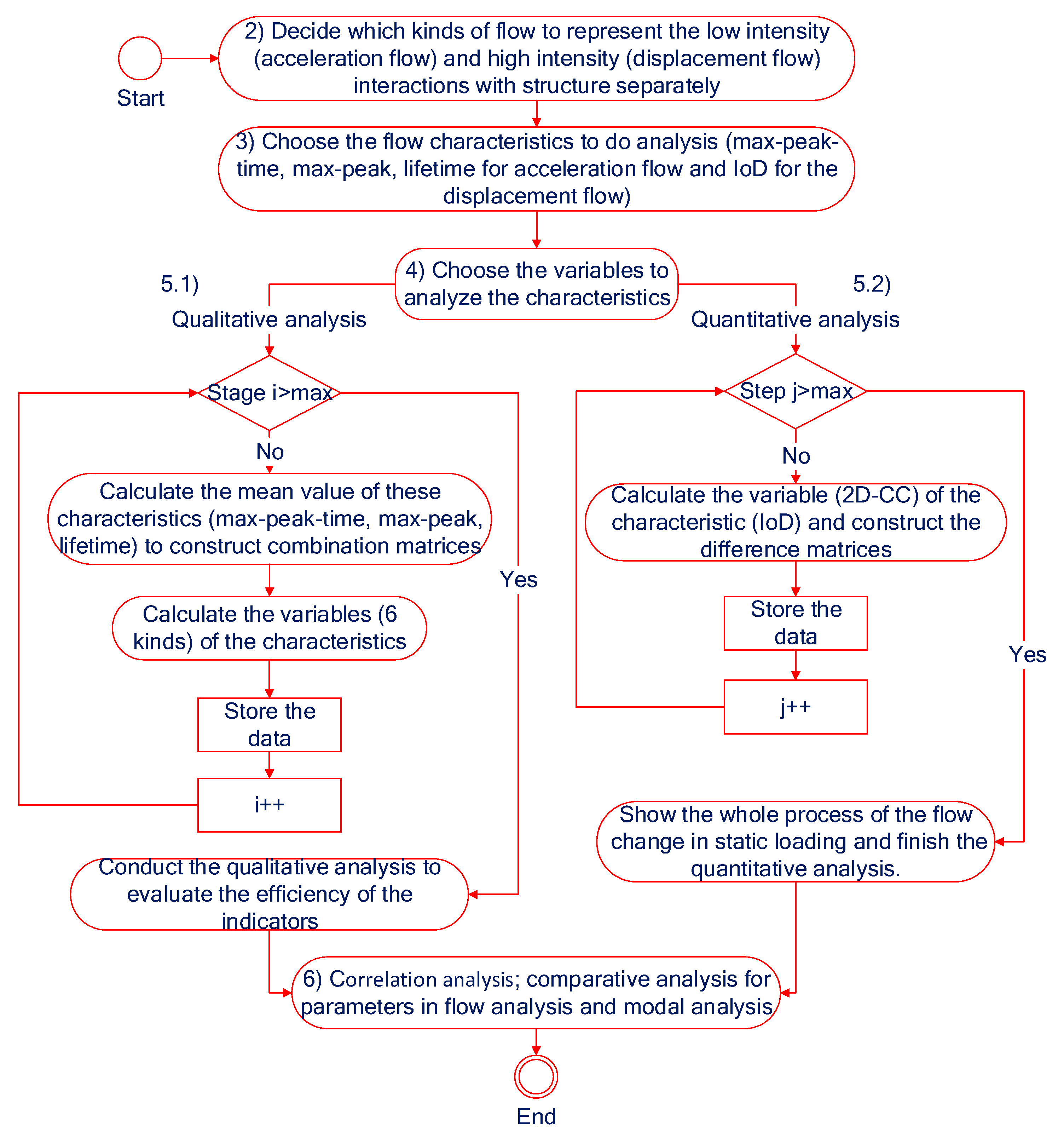
Choose the flows to analyze (in this paper, we choose the displacement flow to represent the flow of high intensity and the acceleration flow to represent the flow of low intensity, respectively).
3)
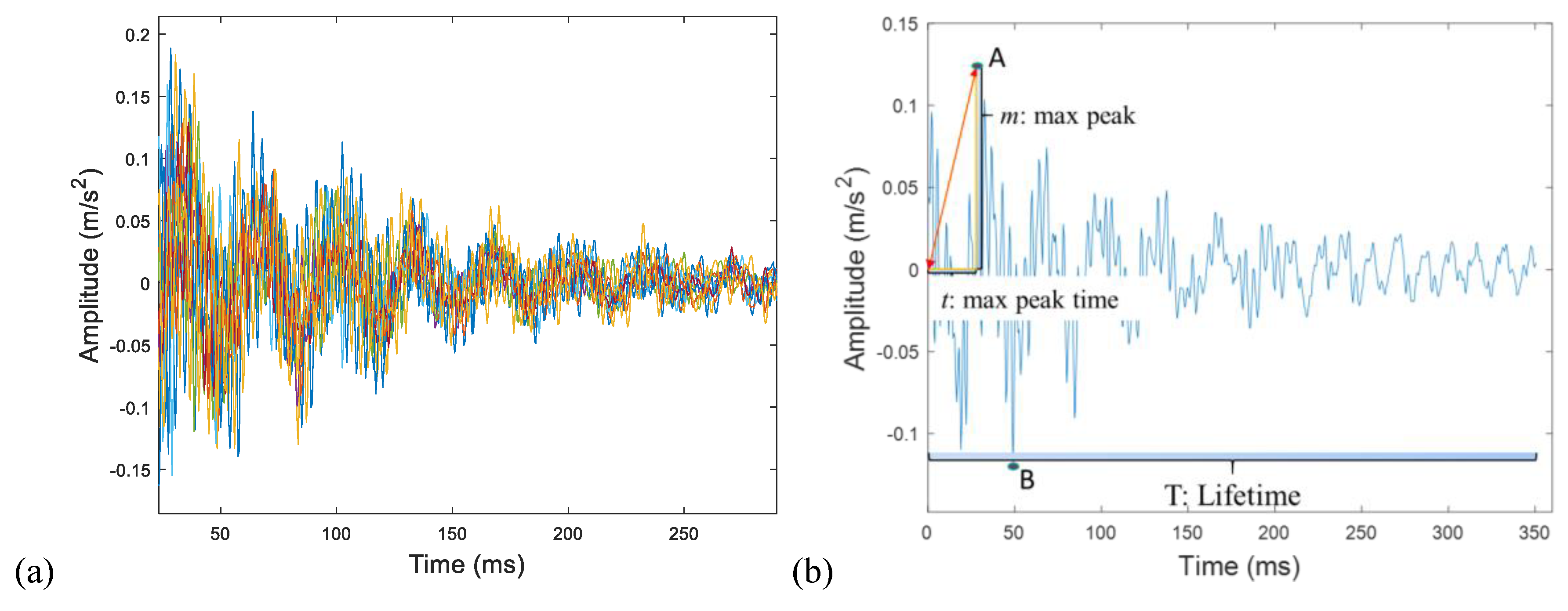
Choose the flow characteristics (max-peak-time from class 1, max-peak from class 3, and lifetime from class 4 are chosen for acceleration flow, and IoD from class 3 is chosen for displacement flow).
4)
Choose the variables to represent the flow’s characteristic matrices (6 kinds of variables will be used in the analysis, in which “determinant, norm, max eigen, 2D correlation coefficient, distance, Procrustes” are for acceleration flow and “2D correlation coefficient” is for displacement flow).
5)
Data analysis.
5.1)
Do the qualitative analysis for the acceleration flow. There are 9 stages (maximum amount = 9) in this data processing. Calculate the expectation of characteristics from the times recorded by different acceleration sensors. Construct the combination matrices. Calculate the variables to evaluate the characteristics. Conduct the qualitative analysis.
5.2)
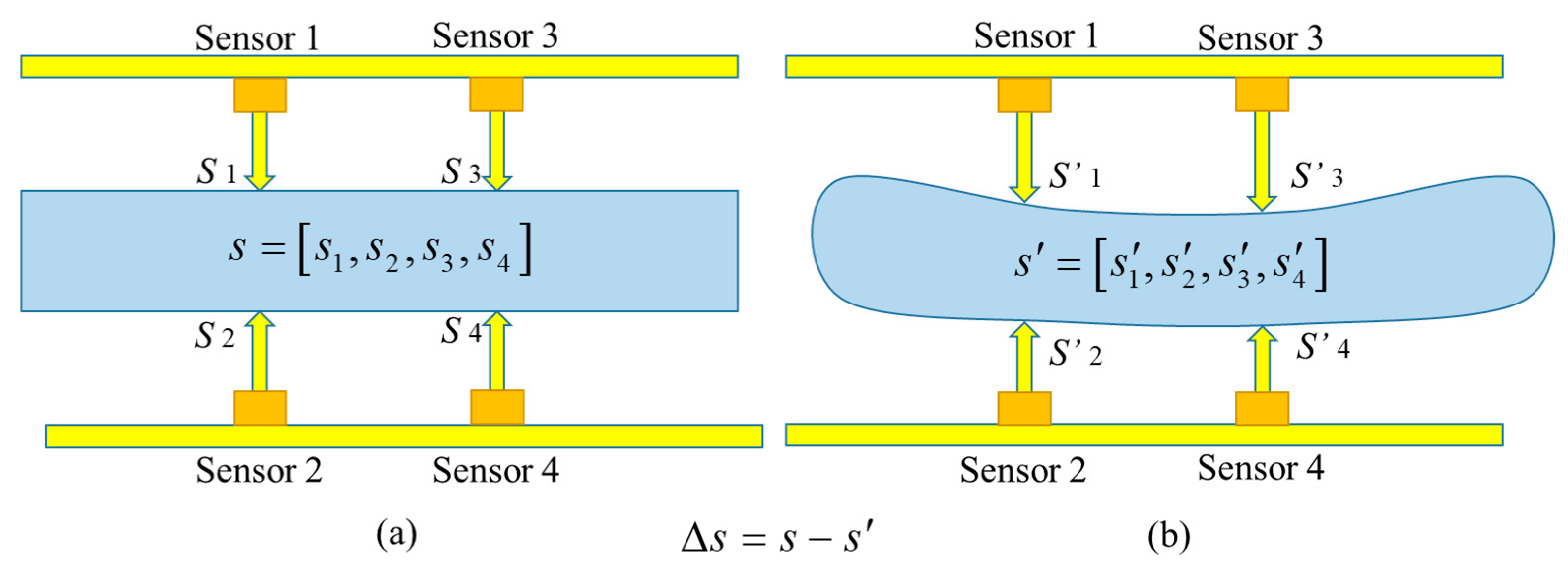
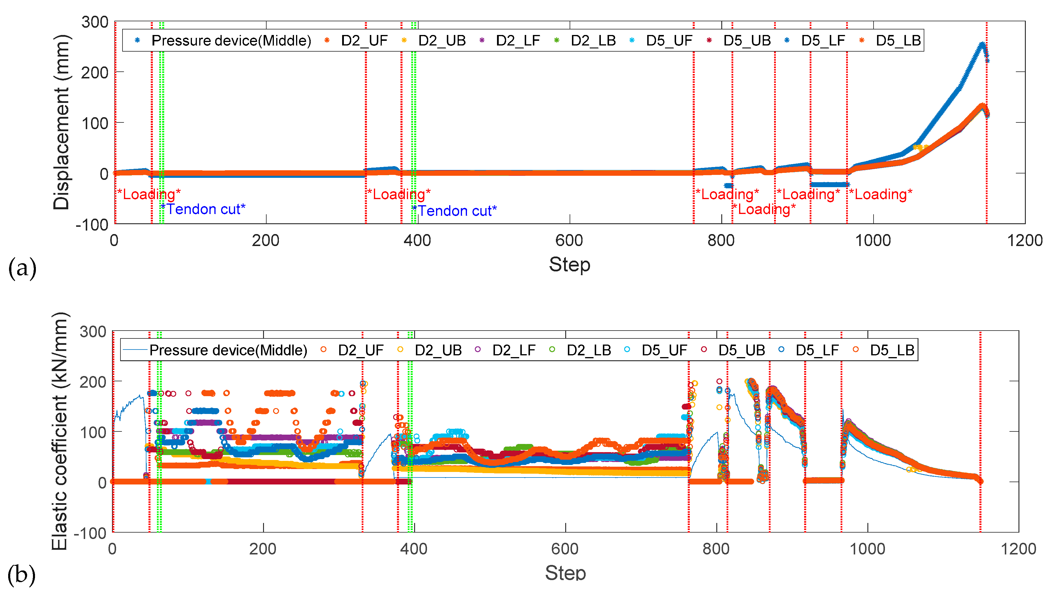
Do the quantitative analysis for the displacement flow. There are 11 stages (maximum amount = 11), or more than 1000 steps in this data processing. Collect the data recorded by different acceleration sensors at the same moment as arrays (loading ID, step). Construct the difference matrices. Calculate the variable (2D-CC) to evaluate the characteristics. Conduct the quantitative analysis.
6)
Conduct correlation analysis and comparative analysis with modal analysis.
6.1)
Calculate the correlation coefficient and conduct the correlation analysis for kinds of flow characteristics.
6.2)
Compare the (acceleration) flow characteristics with the structural characteristics in modal analysis. These characteristics of both flow and structure all are using the same original data.
7)
End of the data analysis.

4. Results and Discussions

4.1. Calculation Method of Variables for Characteristics Matrices

In the experimental data processing, some variables used to describe the characteristic matrices may change from the former stage to the latter stage in the structural artificial lifetime:
M initial = [ x 1 , 1    x 1 , 2       x 1 , j       x 1 , a x 2 , 1    x 2 , 2       x 2 , j       x 2 , a                x i , 1    x i , 2       x i , j       x i , a                x b , 1    x b , 2       x b , j       x b , a ] M considered = [ x ¯ 1 , 1    x ¯ 1 , 2       x ¯ 1 , j       x ¯ 1 , a x ¯ 2 , 1    x ¯ 2 , 2       x ¯ 2 , j       x ¯ 2 , a                x ¯ i , 1    x ¯ i , 2       x ¯ i , j       x ¯ i , a                x ¯ b , 1    x ¯ b , 2       x ¯ b , j       x ¯ b , a ]
Here is an example: A change of numerical value matrix:   [ 1 5 9 6 3 8 10 5 3 ] =>   [ 1 5.4 9.5 7.5 4 6.3 10 4 2.5 ] and its numerical order change: [ 1 2 3 2 1 3 3 2 1 ] => [ 1 2 3 3 1 2 3 2 1 ] . The results for both the order matrix and value matrix of determinant, norm, max eigen, 2D-CC, distance, and Procrustes are shown in Table 3 and Table 4.
Just as the example above indicates, the value of each variable has changed from the initial stage to the second stage (named the considered stage) in both value and order according to the categories in Section 3.2. Even though the initial order matrix can be directly derived from the ideal state, it is still hard to guarantee the same effectiveness in practice. It is found in this example that the value matrix has a higher sensitivity than the order matrix, and the comparison variables have higher sensitivity than the intrinsic variables. However, since the sensitivity is too high in some cases, the data tend not to show the signs of change.

4.2. Quantitative Study of the Displacement Flow

In this section, 2D-CC is used to show the similarity [43] between the reference matrix (in the initial health stage) and some considered matrix (in the considered stage), describing the change of the IoD in displacement flow within a very clear range of [−1,1].
Comparing Figure 9 and Figure 10 with Figure 11 and Figure 12, Figure 9a and Figure 11a show the original data of the “displacement VS step” of box girder 2 and box girder 3, respectively; Figure 10 and Figure 12 show the analysis results using 2D-CC for the difference matrices of IoD of displacements detected by meters (D2_UF, D2_UB, D2_LF, D2_LB, D5_UF, D5_UB, D5_LF, D5_LB) corresponding to the Figure 9a and Figure 11a, respectively.
Comparing Figure 9a with Figure 10 and Figure 11a with Figure 12, the variable of 2D-CC calculated according to Equation (7) is more sensitive than the displacement itself. In these figures, the reference matrix (initial) is set as some difference matrices at approximately 2–5% design load. From Figure 9a and Figure 11a, the relationship between the loads and the structure response (displacement) is very clear in that in the experiment, when the loads on the structure increased, the displacement of the structure increased as well. However, for more detailed information in the whole experimental process, it is a little harder. Comparing Figure 9b with Figure 10 and Figure 11b with Figure 12, it is known from the basic knowledge of structural mechanics that under a static load, if the basic shape is assumed to have not changed, the force applied to each part of the structure will be proportional to the force exerted by the loading device. Therefore, in Figure 9b and Figure 11b, the elastic coefficient is calculated by k = F/s, where F is the force of static loading and s is displacement, and it is not necessary to calculate the forces at different positions. The main change in this study is the plasticity change, so the elastic coefficient is always changing in the static loading experiment. After taking the absolute value, the elastic coefficient of the structure itself undergoes a series of changes without loading after tendon cut, which is consistent with the results obtained by flow analysis. This process is a rebalancing process of the structure, which is the restabilization of the structure itself under gravity after the tendon cut. Moreover, even the asymmetric temperature can also influence the redistribution of structural internal force [44].
In detail, in Figure 10 and Figure 12, for stages 2, 5, and 8–11 of static loading, the difference matrix of displacement detected by different meters in different locations of the structure may slowly change, since the loading increases on the structure and the 2D-CC decreases; since the damages have occurred differently, the 2D-CC can still be maintained at a stable level after the static loading experiment. Once the loading disappears, there is a sudden but great change. For the 3rd and 6th stages of tendon cut, the 2D-CC changes suddenly, signifying the severe redistribution of internal force in the structure. Since the damage increases from the 3rd stage to the 6th stage, the reaction of the 6th stage will be more severe. From the 2D-CC of the intensity distribution, every time after the tendon cut, there is a short time in which the structure can migrate to a new balance (a new development of the artificial damage and a new resistance condition), and the flow in the system will change with high uncertainty. For the 4th and 7th stages of the recovery period (almost 3 days) after the tendon cut, from comparing Figure 10 with Figure 12, it is very clear that different kinds of tendon cut will have different results. In the result of box girder 2, from the tendency in Figure 10, just after the tendon cut, suddenly, the 2D-CC of the difference matrix increases, which means the structure may have an enhancement within a short time, and perhaps the structure releases some of its residual resistance at once. Then, the structure will be in a series of changes of alternating cycles, enhanced or weakened, and then achieve new balances. There are two shapes of “W” in both recovery periods of 3 days, and the 2D-CC experiences 5 recovery stages. For the reason that the difference matrix S shows the difference of displacement detected every two meters, it can be used in a variety of transferring equilibria of the displacement swarm (detected by different meters) in the structural artificial lifetime. Since in the asymmetric cut of C1, C2, and C3 in box girder 2, there are 3 equilibria transferring, there exists a “far from equilibrium state” according to dissipative structure theory, such as the change of recovery stage 2 and recovery stage 4 as seen in Figure 10. Meanwhile, in Figure 12, the box girder 3 is symmetrically cut, and from the original data, it may not be easy to find such kind of changes. About this phenomenon, from the perspective of flow analysis, it may contain the linear change near the real balance state, i.e., the so-called “near equilibrium state”. After the tendon cut, the change of the system is possibly influenced by the action of environmental micro-perturbation, where the crack or the weak part in the structure slowly crept so that the structural damage occurred and developed in different locations, but due to the asymmetry of the tendon cut, the 2D-CC of the difference matrix can clearly indicate the damage effect for that the reference (initial) matrix is designed based on the initial symmetry structural state.
In summary, since the test beams have the symmetrical size and commonly used type in the field, the damage detection based on 2D-CC of the characteristic of the displacement flow can investigate the continuous damage caused by the static loading and the tendon cut. Especially for the tendon cut, the special “W” shape is clearly seen.

4.3. Qualitative Study of the Acceleration Flow

The qualitative study involves an understanding of a phenomenon, situation, or event which comes from exploring the totality of the situation [45]. In this study, the impact hammer experiment was carried out manually. It is almost impossible to collect raw data continuously in all loading instants, so flow analysis can only be conducted discretely at nine major stages. The results of limited stages can only give a trend to approximate the damage changes in the structural artificial lifetime. So, in the flow analysis for the impact hammer experiment, the qualitative study is the mainstay, supplemented by the quantitative study to evaluate this trend. Further, inspiration is taken from the tendency of stock market research or other fields, where an average directional index (ADX) or directional movement index (DMI) is an indicator used in technical analysis as an objective value for the strength of a trend [46], wherein one kind of qualitative directional index (QDI) is proposed to identify the effectiveness of the methods. When comparing the reasonable development tendency and the analytic result, every change of forward and backward development will be defined by +1 and −1, respectively.
QDI was calculated as follows: First, in a sequence, from one point to the next point, if the derivative (or value of the post value minus the previous value) of the broken line is positive, the value of change is “+”; if the derivative of the broken line is negative, the value of change is “−”; if the derivative (ki, i = 1,2,3,…,N) of the broken line is 0 or near 0 ( | k i | / | k i + 1 | ε ,   i = 1 , ( | k i | / | k i + 1 | ε ) ( | k i | / | k i 1 | ε ) ,   i = 2 , 3 , 4 , , N 1 , and | k i | / | k i 1 | ε ,   i = N ), where | k i 1 | , | k i | , | k i + 1 | are three adjacent derivative values and ε is a very small number, or usually just according to the resolution of the naked eye on figures or curves), the value of change is 0. Second, according to the QDIs of all variables of characteristics (sum of data, whose absolute value should be not less than γ , and γ in this paper is 2/8) of the tendency, delete the result which cannot be clearly distinguished. Then, assign the weight: For the order, 1, and for the value, 3. Meanwhile, get the sum of these value, and if it is positive, it is +1, and if negative, −1. Last, get the accumulation of the value over the total number of stages. For example, for the approximate steps in 2D-CC of IoD matrices for the time in different stages of the impact hammer experiment (Figure 13), its QDI is 6/8.
The indicators show the same tendency of damage development in the two girders using different kinds of variables. Take the 2D-CC, for instance. The characteristic matrices are introduced in Section 3.1, M, in which xi,j is the expectation of characteristic values of time series at one hit point.
All characteristics and variables to describe the characteristic matrices are analyzed by qualitative study, and the results are summarized in Table 5 and Table 6. In Table 5b, since the determinant, distance, and Procrustes will increase, here, we just multiply it by −1 in the results of these variables. In Table 6b, since the determinant, distance, Procrustes will increase, here, we just multiply it by −1 in the results of these variables.
The final QDI of the acceleration flow described by these characteristics and variables are 3/8 (by variables) and 4/8 (by characteristics) in Table 7 (referring Table 5a and Figure 13), respectively. Surveying these tables, different characteristics have different sensitivities to reveal the tendency of damage development; from Table 6, the max-peak-time has the best results from three selected characteristics. Overall, there are many equilibrium states of flow (stages 1–2, stages 2–7, and stages 7–9) from Figure 13 and Table 5 and Table 6 and at stage 2 and 7, there are large balance equilibria migrations, such that various characteristics will have larger differences than other stages.
Generally, but not strictly, [0, 0.3) means no correlation, [0.3, 0.5) is a weak correlation, [0.5, 0.8) is moderate correlation, and [0.8, 1.0] is a strong correlation. From Table 8 and Table A2, the coefficients of the sequence correlation between every two characteristics of acceleration flow have many strong relationships. Since the correlation coefficient is related to cosine similarity [47], it also shows that the different intensity of flow will have different responses of structure in Section 2.2. In the experimental data analysis, different from the data (the IoD) obtained from the static loading experiment (displacement flow), the data (max-peak-time, max-peak, and lifetime) obtained from the impact hammer experiment (acceleration flow) shown in Figure 10 only had a weak correlation in the tendency of change. However, from observation of the curve in Figure 13 and Figure 14, the QDI of displacement flow with 2D-CC is superior to any characteristic of acceleration flow in the impact hammer experiment with only 2D-CC in numerical value.
In summary, the damage indicators using flow analysis provide a new study of damage assessment. Although the results are not yet perfect, it is still possible to find that if the appropriate variables and characteristics are selected, satisfactory results can be obtained.

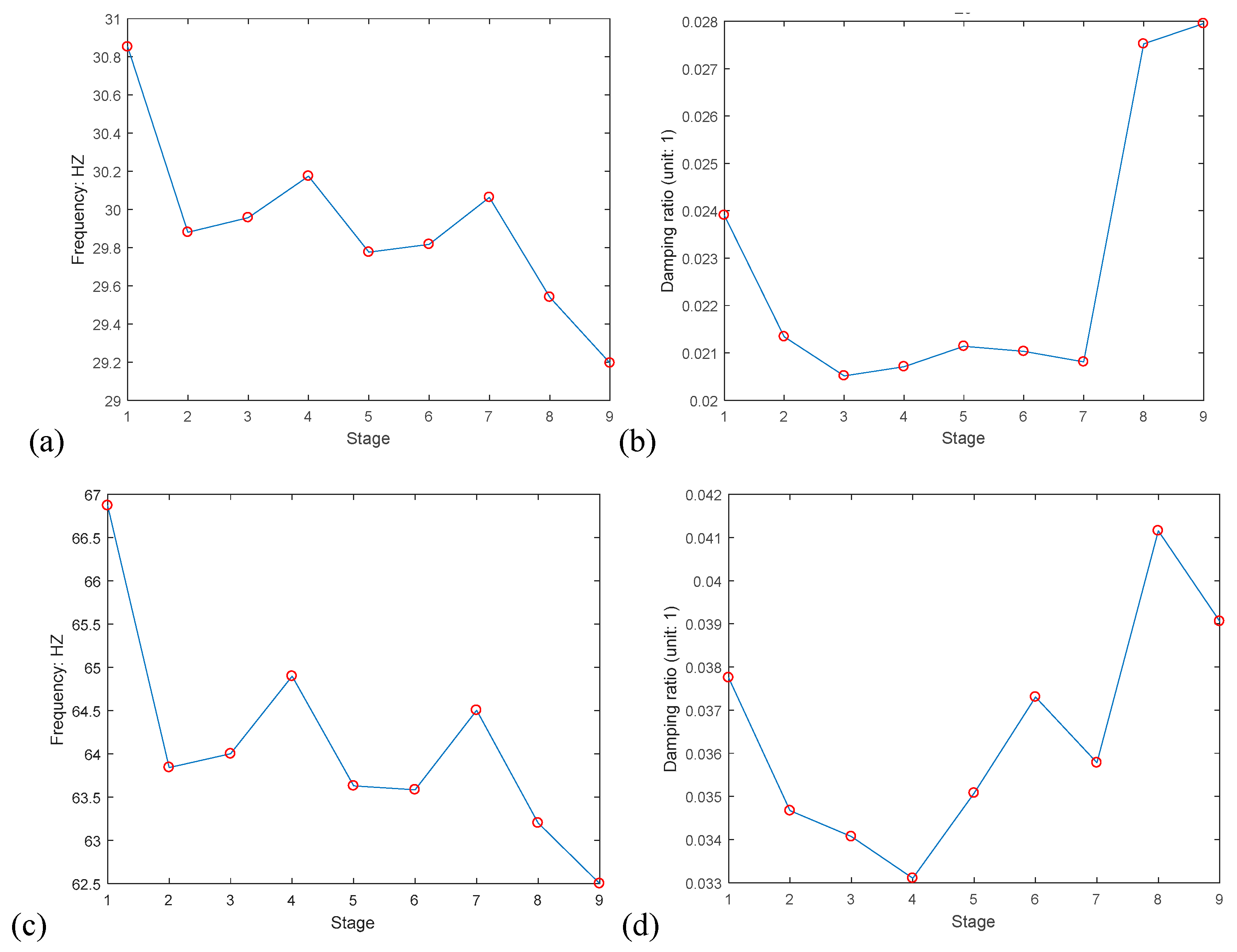
4.4. Comprehension between Flow Characteristics and Structural Dynamic Characteristics

The modal analysis and flow analysis can both be data analysis tools (Table A1), but even when analyzing the same data, they interpret structure and flow characteristics differently. Using the same data as the flow analysis, from the previous research, in all modes of modal analysis, the frequencies of lower modes (e.g., the 1st and 2nd bending modes in Figure 15 and Figure 16 using stochastic subspace identification (SSI)) may be adequate to evaluate the structural damage degree. The QDIs of both modes are shown in Table 9 and Table 10.
When the artificial damage gradually increases in the structure, the internal forces were redistributed, such that the cracks may be wider, deeper, and longer; the relationship between substructures may change; and the rate of energy dissipation may vary. The strength of associations among substructures will directly affect the occurrence and development of cracks. Then, the flow in the system may have different routes and rates of dissipation. There are some assumptions or presuppositions:
  • Once the crack has emerged, it will not disappear, and the depth and length will not shrink.
  • The redistribution of internal forces will change the strengths of associations among substructures as well as the width of cracks.
  • In statics, the energy dissipation is depending on the length of the route that the flow goes.
  • The natural frequency is determined by the structure itself, and the elastic modulus or coefficient of stiffness will directly influence the change of the natural frequency. Natural frequency in the experimental data processing using SSI is a holistic concept of the structure.
  • Global change is determined by the sum of the local changes.
In practice, the material characteristics of some systems are often nonlinear and nonstationary (for instance, the concrete box girder), and thus some structural characteristics may be ineffective. Further, the flow analysis of acceleration flow can be effective using the same original data of the modal analysis.
Comparing the results between modal analysis and flow analysis in Figure 14 and Figure 16, and from the qualitative study in Table 5, Table 6, Table 9 and Table 10, some observations can be made as follows: In the experiment, the overall size of the structure does not change visually, while the sizes of the existing cracks or new cracks, with their continuous development, will have undergone tremendous changes. From the results, the flow characteristics are more sensitive to the cracks’ depth and length, while the structural characteristics through modal analysis are more sensitive to the redistribution of forces or the width of the cracks; both are specially related to the topology of the flow channel in class 2 of flow characteristics. That is to say, despite the topology of the channel being hard to obtain, its change will bring about the change of max-peak and max-peak-time in other classes of characteristics (1st and 3rd) and the structural characteristics. Among three kinds of flow characteristics, the max-peak and max-peak-time are relating to the change of “flood” of flow and the change of the flow’s main part, respectively, while the lifetime is related to the whole process of the flow change in the structure. Put another way, the energy dissipation in the structure from the locations of input to the locations of output in the impact hammer experiment will follow different paths. When there is max flow (the max magnitude), it means there are “floods” in some locations.
As the natural frequency changes in Figure 16 shows, the coefficient of stiffness has changed for the reason of cracks change. To sum up, the natural frequency and the “max-peak and max-peak-time” have relatively strong coefficient correlations in Table 11. In Figure 16, in the process of every tendon cut and recovery after tendon cut (from stage 3 to stage 4 and from stage 6 to stage 7), the force may be redistributed again, the specific prestressing design leads to an increase in the elastic modulus of many positions, and the crack width becomes smaller, resulting in an increase of the low-order natural frequency and a decrease of the damping ratio. Through observation, the flow characteristics of max-peak and max-peak-time are not sensitive to the width of the cracks, thus they would not change abnormally. Concerning the damping ratio and the lifetime, they share the same idea that the intensity of the wave gradually decreases. In the assumption, the global change is determined by the sum of the local changes; one the one hand, the stiffness coefficient varies in different locations and differs from the global one, in that the different integrated methods (such as the modal parameters) will give different results, which will not correctly reflect the real damage of the structure; on the other hand, the flow analysis combined almost all original data space (data recorded at the surface of the structure) in different locations to investigate the change of public information and it can help get the result with higher precision. Furthermore, if we concern all kinds of structural characteristics, as well as many kinds of flow characteristics simultaneously, some better results may be obtained in the analytic hierarchy process.
In summary, through evaluating the order matrix and value matrix in flow analysis, both the intrinsic variables and comparison variables in different stages outperformed the modal characteristics (frequencies and damping ratios). By analyzing the correlation of two methods, it is obvious that both complement each other. If they are used in conjunction, some better structural damage assessment may be achieved, and then multi-criteria decision-making [48] can be conducted.

4.5. Measurement, Sampling, and Error

Generally, in order to know the behavior of flow in the structure, we measure the flow of import–export through the structure to indirectly assess the interaction (described as the dynamical field) between structure and environment. Moreover, this interaction can be formed between structure and flow, as well as between flow and environment. Further, in a global system, the measured data (often in time series) often contain information of structure, flow, and environment at the same time. For instances, for a time series, the natural frequency can be obtained from the modal analysis, the flow characteristics can be obtained from flow analysis, and some environmental characteristics can also be obtained from the error analysis, even when the whole environment is well controlled (e.g., in indoor experiments). Furthermore, every measurement might carry environmental update information. So, based on our assumption, inherent error analysis can also be partly treated as environmental analysis, although the experimental condition is strictly controlled in this indoor experiment.
In the data analysis, it is difficult to avoid some errors. To explain the reasons for these errors, besides the influence of the environment and random error of measurement, there are inherent errors in the data itself. Here, to explain the data accuracy, two possible reasons in this section are discussed.
Firstly, the arising phenomenon that causes the insufficient sampling rate of the experiment results is limited by the instrument [49].
Secondly, the assumed ideal situation and the situation in practice are sometimes totally different or the measurement error is so great that the information we want is hard to distinguish. In the construction and conservation period, this girder has experienced kinds of interactions with the environment, but also its own structural defects, and maybe there are numerous microcracks in the structure that cannot be observed with the naked eye, so the inner condition is not ideal.
Following is a pair of order matrices for acceleration flow with 7 input locations and 7 output locations in the initial stage: Real measurement versus the ideal situation (experiment in Figure 17):
[ 2 3 1 4 5 6 7 2 3 1 4 6 7 5 3 4 2 1 7 5 6 2 6 3 4 1 5 7 5 6 4 3 2 1 7 6 5 4 7 2 1 3 4 1 2 7 5 6 3 ]   VS .   [ 1 2 3 4 5 6 7 2 1 , 3 3 , 1 4 5 6 7 3 2 , 4 4 , 2 1 , 5 5 , 1 6 7 4 3 , 5 5 , 3 2 , 6 6 , 2 1 , 7 7 , 1 5 4 , 6 6 , 4 3 , 7 7 , 3 2 1 6 5 , 7 7 , 5 4 3 2 1 7 6 5 4 3 2 1 ]
For one input location, there may firstly be two possible sensors to detect the same prescriptive signal at the same time. For example (red font in the matrix above), for the input at hit 2, sensors 1 and 5 may detect this signal at the same time, but in the real measurement, either sensor 1 or 5 would detect the signal earlier rather than the two sensors detecting it at the same time.
Furthermore, in the quantitative study for the displacement flow, the unique data do not have statistical meaning. In the qualitative study for the acceleration flow, only investigating the expectation in statistics cannot provide the continuous and comprehensive change of the structural artificial lifetime. Further, in some cases, human error may also bring about some strange or wrong results. Fortunately, in this paper, the summarized results have a clear trajectory of change, which is enough to approximately show the overall change of the structure, and these indicators in flow analysis can be used to demonstrate the damage development.

4.6. The Application of the Flow Analysis in Practice

To apply the indicators of flow analysis to damage identification, there are several concerns, as follows.
First, the characteristics for decision-making should be carefully chosen. For different kinds of flow, how to select these characteristics properly depends on the structural types, materials, environment, and so on as well as the measurement practicability. Second, the experiment (detection or monitoring) should be well organized so that the data can carry enough information about the structure and flow. Third, if possible, multiple kinds of flow should be considered, which can aid in better analysis and comparison in practice. Last, besides flow analysis, other kinds of methods can also be conducted to help decision-making.
For the damage caused by static loading, if a structure is damaged, the structural equilibrium state may change. For example, in our case, about the quantitative study of the displacement flow, in stage 2, the structure firstly suffers a heavy loading and its inner structural rebalance occurs; after the loading, a permanent change appears in the curve “2D-CC versus step”. Moreover, after static loading in stage 7, the 2D-CC is near or smaller than 0, so the system becomes totally different from its formal equilibrium and there is a high likelihood that the structure has experienced great damage. Further, in the discussion about the qualitative study of the acceleration flow, there are 3 equilibria. The first equilibrium is from stage 1 to stage 2. The second equilibrium is from stage 2 to stage 7. From stage 2, the structure has suffered a series of changes, for which almost all the indicators tend to be in disorder of complex curve-changing to a certain extent. The third equilibrium is from stage 7 to stage 9. After stage 7, the change of all variables describing reunification of all characteristics occurs, indicating that the structure may suffer a strong weakening. In practice, if there is an anomalistic change for all curves of indicators, it means there is an equilibrium shift of flow and there may be a great damage in the structure such that it asks the decision-maker to pay more attention to whether there is a need to maintain the structure.
In the tendon-cut damage case, the broken tendon is mostly asymmetrical in real structures. In our research, it is shown that an asymmetrical tendon cut will have a serial of rebalances in the structure and that the flow in the structure will have a large number of states far from equilibrium in the vicinity of the equilibrium state, and finally, a new balance will be formed. This kind of special change will be used to indicate the tendon breakage or not. The tendon here is cut at the end. More experiments should be done, as there may exist different kinds of modes when the tendons are broken in different ways or locations of prestressed structures.
Further, only concrete box girders were tested in this study. More tests should be conducted with other styles of structures and damage.
Fortunately, according to the dissipative structure theory, all structural changes follow the same law in system theory on equilibrium state migration. Meanwhile, if there is a big change in the structure, the efficient indicators can identify such changes as well. Since the flow exists in every system and the change of structure is just reasoned as the interaction between the structure and the flow, then the flow characteristics should have some changes corresponding to the changes in the structure.
The experiment method applying flow analysis can also be used in the common health monitoring of bridges or other structures, such that the curve of the flow characteristic may have a clearer and more continuous tendency. For the real bridge, for the displacement flow, the damage caused by tendon cut and the loads (vehicles or humans) can be detected by a swarm of meters. For the acceleration flow, it may use the data of vibration caused by wind, rain, or interaction between bridge and vehicles to show the change of flow in different characteristics. The arrangement of sensors can be decided according to the specific problem, and the data style can be varied in practice. Besides this research, to use the flow analysis with the data obtained by other methods, the data should be well organized into swarm data. Then, the reconstructed data matrix or some other form of data may be used in flow analysis.

5. Conclusions

In the global structural system, the interaction between structure and environment can be transformed into the interactions between structure and flow and between flow and environment; the interaction among substructures can be transformed into the interaction between flow and substructures. Flow can destroy the structure and can also be used to evaluate the structure. Often, but not strictly, a strong flow might damage structures, while a weak flow can be used to detect the existence and the level of damage. The flow analysis is mainly about the stability of flow characteristics. By evaluating the change of these characteristics, it is possible to assess the damage of the structure when the structural condition changes.
The flow analysis defines a system as a dissipative structure, utilizes the combined data space, provides a general description (usually matrices) of the system, and compares the similarity among different system development stages which can precisely identify the minor changes in the system. Kinds of flow characteristics can have relatively clear tendencies in the artificial structural lifetime, which indicates that the flow characteristics can be used to evaluate the structure indirectly with a higher QDI than some structural characteristics in the modal analysis with higher sensitivity in the damage diagnosis.
The main experiment objects are two nearly full-scale girders, investigations of which have been rarely conducted in past studies. In the experiment, two kinds of information flow were investigated in data analysis: Displacement flow and acceleration flow. The continuous aggravating damage was applied to the structure in different stages. In this process, the change of the flow characteristics can approximately indicate the tendency of the increasing damage, while some modal parameters (in modal analysis) failed to distinguish the change of structure, which shows the swarm behavior of displacement and the swarm behavior of waves, indicating the multistage redistribution of force and cracks in the structure.

Author Contributions

Conceptualization, X.-F.Y.; methodology, X.-F.Y.; validation, X.-F.Y., C.-W.K. and K.-C.C.; formal analysis, X.-F.Y., K.-C.C.; investigation, X.-F.Y.; resources, O.S.L.V., Y.O.; data curation, X.-F.Y.; writing—original draft preparation, X.-F.Y.; writing—review and editing, X.-F.Y., K.-C.C., C.-W.K., H.O., Y.O., O.S.L.V.; visualization, X.-F.Y.; supervision, C.-W.K., H.O.

Funding

This research received no external funding.

Acknowledgments

The first author would like to express his appreciation for the support from the China Scholarship Council in both life and research. This study was partly supported by a Japanese Society for Promotion of Science (JSPS) Grant-in-Aid for Scientific Research (B) under Project No. 16H04398. That financial support is gratefully acknowledged.

Conflicts of Interest

The authors declare no conflict of interest.

Appendix A

Table A1. Wave characteristics for damage diagnosis.
Wave Characteristics (Flow)Damage Diagnosis
Sound (Voice, Song)Wave (Flow)Analyzing Methods Data Processing
LoudnessAmplitude/wavelengthFlow characteristics,
Structural characteristics,
etc.
Frequency response,
Time–history response,
etc.
Extreme analysis,
pattern recognition,
analysis of similarity/difference, etc.
The data in flow analysis are often in a matrix, evaluated by determinant, norm, max eigen, 2D correlation coefficient, distance, and Procrustes;
for statistics: expectation,
variance, mode, median;
For other data forms, there are some other evaluation methods.
Acoustic pressureDistance, sound pressure or intensity, damping
Auditory impressiondirection and speed of sound (velocity)
ToneFrequency
Musical sound or noiseHarmonic wave
TimbreWave pattern
Pitch intervalWave interval
Concerto, SymphonyPrincipal component analysis, association analysis, etc.
Table A2. The characteristics of modal analysis and flow analysis.
MethodStageStage 1Stage 2Stage 3Stage 4Stage 5Stage 6Stage 7Stage 8Stage 9
Modal AnalysisFr_2930.852029.880129.957330.174729.776129.817330.063129.540329.1955
Fr_6566.870363.842864.000564.897663.630363.585364.504263.201262.5008
DR_29−0.0284−0.0241−0.0229−0.0240−0.0238−0.0242−0.0240−0.0311−0.0314
DR_65−0.0493−0.0486−0.0502−0.0474−0.0496−0.0535−0.0492−0.0584−0.0577
Flow Analysis
using
2D-CC
IoD1.00000.73680.72230.60590.61990.28110.56120.1408−0.3431
Max-peak1.00000.79290.79510.77220.65940.71460.71840.72390.6980
Max-peak-time1.00000.94530.93590.94610.94530.94560.92230.93990.9467
Lifetime1.00000.19360.21280.25120.0047-0.02760.25020.44850.3660
Note: Fr_29 and Fr_65 denote the frequency around 29 Hz and 65 Hz, respectively, while DR_29 and DR_65 are the damping ratios corresponding to frequency around 29 Hz and 65 Hz, respectively. Flow analysis (2D-CC) is applied on the difference matrix of IoD of displacement flow and the value matrix of max-peak-time, max-peak, and lifetime of acceleration flow.
Figure A1. Simulation by the Lattice Boltzmann method (LBM) for the flow in the space in different stages (A, B, C, and D), in which A1, B1, C1, D1 simulate the line–crack barrier, while A2, B2, C2, and D2 simulate the round hole barrier. The flow is imported into the system with a limited boundary continuously.
Sustainability 11 00710 g0a1
Note for Figure A1: There are three basic methods to simulate the flow for different fineness: the graph method and element method (finite element method, FEM, and boundary element method, BEM, etc.), responding to the macroscale or LBM (Lattice Boltzmann method) responding to mesoscale (multiscales); and the field method, responding to the microscale. Based on the element method and LBM, the flow in systems can be shown up figuratively. Further, the graph method is often used in the search for the propagation path for energy flow in structures or systems that have clear boundaries, and the method using field theory to describe the flow more mathematically, which is an important aspect in fluid mechanics, wind mechanics, gravitation, and geomagnetics, etc.

References

  1. Enright, M.P.; Frangopol, D.M. Survey and evaluation of damaged concrete bridges. J. Bridge Eng. 2000, 5, 31–38. [Google Scholar] [CrossRef]
  2. Okeil, A.M.; Cai, C.S. Survey of Short and Medium-Span Bridge Damage Induced by Hurricane Katrina. J. Bridge Eng. 2008, 13, 377–387. [Google Scholar] [CrossRef]
  3. Watanabe, E.; Furuta, H.; Yamaguchi, T.; Kano, M. On longevity and monitoring technologies of bridges: A survey study by the Japanese Society of Steel Construction. Struct. Infrastruct. Eng. 2014, 10, 471–491. [Google Scholar] [CrossRef]
  4. Ph Papaelias, M.; Roberts, C.; Davis, C.L. A review on non-destructive evaluation of rails: State-of-the-art and future development. Proc. Inst. Mech. Eng. Part F J. Rail Rapid Transit 2008, 222, 367–384. [Google Scholar] [CrossRef]
  5. Bayraktar, A.; Türker, T.; Tadla, J.; Kurşun, A.; Erdiş, A. Static and dynamic field load testing of the long span nissibi cable-stayed bridge. Soil Dyn. Earthq. Eng. 2017, 94, 136–157. [Google Scholar] [CrossRef]
  6. Song, W.; Chunguang, X.U.; Pan, Q.; Song, J. Nondestructive testing and characterization of residual stress field using an ultrasonic method. Chin. J. Mech. Eng. 2016, 29, 365–371. [Google Scholar] [CrossRef]
  7. Stepanova, L.; Roslyakov, P. Multi-parameter description of the crack-tip stress field: Analytic determination of coefficients of crack-tip stress expansions in the vicinity of the crack tips of two finite cracks in an infinite plane medium. Int. J. Solids Struct. 2016, 100, 11–28. [Google Scholar] [CrossRef]
  8. Prigogine, I. Moderation et transformations irreversibles des systemes ouverts. Bull. De La Cl. Des Sci. Acad. R. Belg 1945, 31, 600–606. [Google Scholar]
  9. Nicolis, G.; Prigogine, I. Self-Organization in Nonequilibrium Systems; Wiley: New York, NY, USA, 1977. [Google Scholar]
  10. Prigogine, I.; René, L. Theory of dissipative structures. In Synergetics; Vieweg+ Teubner Verlag: Wiesbaden, Germany, 1977; Volume 1973, pp. 124–135. [Google Scholar]
  11. Jeong, S.; Hou, R.; Lynch, J.P.; Sohn, H.; Law, K.H. An information modeling framework for bridge monitoring. Adv. Eng. Softw. 2017, 114, 11–31. [Google Scholar] [CrossRef]
  12. Khajavi, R. A novel stiffness/flexibility-based method for euler–bernoulli/timoshenko beams with multiple discontinuities and singularities. Appl. Math. Model. 2016, 40, 7627–7655. [Google Scholar] [CrossRef]
  13. Ralbovsky, M.; Flesch, S.D.R. Frequency changes in frequency-based damage identification. Struct. Infrastruct. Eng. 2010, 6, 611–619. [Google Scholar] [CrossRef]
  14. Dammika, A.J. Experimental-Analytical Framework for Damping Change-Based Structural Health Monitoring of Bridges. Ph.D. Thesis, Saitama University, Saitama, Japan, 2014. [Google Scholar]
  15. Pei, C.; Qi, S.; Tang, J. Structural damage identification with multi-objective DIRECT algorithm using natural frequencies and single mode shape. Soc. Photo-Opt. Instrum. Eng. 2017, 10170, 101702H. [Google Scholar]
  16. Manuele, F.A. Hazard Analysis and Risk Assessment. In On the Practice of Safety, 3rd ed.; John Wiley & Sons, Inc.: Hoboken, NJ, USA, 2005; pp. 251–271. [Google Scholar]
  17. Fadeyi, M.O. The role of building information modeling (BIM) in delivering the sustainable building value. Int. J. Sustain. Built Environ. 2017, 6, 711–722. [Google Scholar] [CrossRef]
  18. Bajzecerová, V.; Kanócz, J. The Effect of Environment on Timber-concrete Composite Bridge Deck. Procedia Eng. 2016, 156, 32–39. [Google Scholar] [CrossRef] [Green Version]
  19. Armbruster, D.; Martin, S.; Thatcher, A. Elastic and inelastic collisions of swarms. Phys. D Nonlinear Phenom. 2017, 344, 45–57. [Google Scholar] [CrossRef]
  20. Sagasta, F.; Zitto, M.E.; Piotrkowski, R.; Benavent-Climent, A.; Suarez, E.; Gallego, A. Acoustic emission energy b-value for local damage evaluation in reinforced concrete structures subjected to seismic loadings. Mech. Syst. Signal Process. 2018, 102, 262–277. [Google Scholar] [CrossRef]
  21. Mesnil, O.; Leckey, C.A.; Ruzzene, M. Instantaneous and local wavenumber estimations for damage quantification in composites. Struct. Health Monit. 2014, 14, 193–204. [Google Scholar] [CrossRef]
  22. Wang, T.; Cheng, I.; Basu, A. Fluid vector flow and applications in brain tumor segmentation. IEEE Trans. Biomed. Eng. 2009, 56, 781–789. [Google Scholar] [CrossRef]
  23. Metzger, R.J. The ergodic theory of Axiom A flows. Invent. Math. 2000, 29, 181–202. [Google Scholar]
  24. Gottschalk, W.H. A survey of minimal sets. Ann. Inst. Fourier 1964, 14, 53–60. [Google Scholar] [CrossRef]
  25. Glasner, S. Proximal Flows//Proximal Flows; Springer: Berlin/Heidelberg, Germany, 1976; pp. 17–29. [Google Scholar]
  26. Iseli, A.; Wildrick, K. Iterated function system quasiarcs. Conform. Geom. Dyn. Am. Math. Soc. 2017, 21, 78–100. [Google Scholar] [CrossRef] [Green Version]
  27. Sloan, E.D. Clathrate hydrate measurements: Microscopic, mesoscopic, and macroscopic. J. Chem. Thermodyn. 2003, 35, 41–53. [Google Scholar] [CrossRef]
  28. Wiener, N. Cybernetics or Control and Communication in the Animal and the Machine; MIT Press: Cambridge, MA, USA, 1961. [Google Scholar]
  29. Selleri, F. (Ed.) Wave-Particle Duality; Plenum Press: London, UK, 1992. [Google Scholar]
  30. Shapiro, A.H. The Dynamics and Thermodynamics of Compressible Fluid Flow; John Wiley & Sons: Hoboken, NJ, USA, 1953. [Google Scholar]
  31. Galbis, A.; Maestre, M. Vector Analysis Versus Vector Calculus; Springer: New York, NY, USA, 2012. [Google Scholar]
  32. Reynolds, O. Papers on Mechanical and Physical Subjects, Volume 3, The Sub-Mechanics of the Universe; Cambridge University Press: Cambridge, UK, 1903. [Google Scholar]
  33. Pascal, J.C.; Carniel, X.; Li, J.F. Characterisation of a dissipative assembly using structural intensity measurements and energy conservation equation. Mech. Syst. Signal Process. 2006, 20, 1300–1311. [Google Scholar] [CrossRef]
  34. Von Bertalanffy, L. The theory of open systems in physics and biology. Science 1950, 111, 23–29. [Google Scholar] [CrossRef] [PubMed]
  35. Haag, M.G.; Haag, L.C. The Reconstructive Aspects of Class Characteristics and a Limited Universe // Shooting Incident Reconstruction; Elsevier Inc.: Amsterdam, The Netherlands, 2011; Volume 2011, pp. 35–54. [Google Scholar]
  36. Von Bertalanffy, L. General System Theory; George Braziller, lnc.: Manhattan, NY, USA, 1968; Volume 41973, p. 40. [Google Scholar]
  37. Blanchard, B.S.; Fabrycky, W.J.; Fabrycky, W.J. Systems Engineering and Analysis; Prentice Hall: Englewood Cliffs, NJ, USA, 1990. [Google Scholar]
  38. Hassiotis, S. Identification of Stiffness Reductions Using Natural Frequencies. J. Eng. Mech. 1995, 121, 1106–1113. [Google Scholar] [CrossRef]
  39. Yamaguchi, H.; Matsumoto, Y.; Kawarai, K.; Dammika, A.J.; Shahzad, S.; Takanami, R. Damage detection based on modal damping change in bridges. In Proceedings of the ICSBE’12, Kandy, Sri Lanka, 14–16 December 2013. [Google Scholar]
  40. Ye, X.F.; Ogai, H.; Kim, C.W. Discrepancy Analysis of Load–Displacement in the Combination Space for Concrete Box Girder Assessment. Strength Mater. 2018, 50, 695–701. [Google Scholar] [CrossRef]
  41. Poole, D. Linear Algebra: A Modern Introduction; Brooks/Cole: Boston, MA, USA, 2011. [Google Scholar]
  42. Goodall, C. Procrustes methods in the statistical analysis of shape. J. R. Stat. Society. Ser. B 1991, 1991, 285–339. [Google Scholar] [CrossRef]
  43. Tao, L.; Wang, H.B. Detecting and locating human eyes in face images based on progressive thresholding// IEEE International Conference on Robotics and Biomimetics. IEEE Xplore 2008, 2008, 445–449. [Google Scholar]
  44. Xu, Z.D.; Wu, Z. Simulation of the effect of temperature variation on damage detection in a long-span cable-stayed bridge. Struct. Health Monit. 2007, 6, 177–189. [Google Scholar] [CrossRef]
  45. Ho RT, H.; Ng, S.M.; Ho DY, F. The Sage Handbook of Qualitative Research// The SAGE Handbook of Qualitative Research; Sage Publications: Newcastle upon Tyne, UK, 2005; Volume 2005, pp. 277–279. [Google Scholar]
  46. Chong, O.; Sheng, O. Investigating Predictive Power of Stock Micro Blog Sentiment in Forecasting Future Stock Price Directional Movement. In Proceedings of the International Conference on Information Systems, Icis 2011, Shanghai, China, 4–7 December 2011. [Google Scholar]
  47. Wang, D.; Lu, H.; Bo, C. Visual tracking via weighted local cosine similarity. IEEE Trans. Cybern. 2017, 45, 1838–1850. [Google Scholar] [CrossRef] [PubMed]
  48. Wang, J.Q.; Wu, J.T.; Wang, J.; Zhang, H.Y.; Chen, X.H. Multi-criteria decision-making methods based on the hausdorff distance of hesitant fuzzy linguistic numbers. Soft Comput. 2016, 20, 1621–1633. [Google Scholar] [CrossRef]
  49. Princen, J.; Bradley, A. Analysis/synthesis filter bank design based on time domain aliasing cancellation. IEEE Trans. Acoust. Speechand Signal Process. 1986, 34, 1153–1161. [Google Scholar] [CrossRef]
Figure 1. The relationship of a possible diagrammatic sketch between flow intensity and the structural response which directly influences the observability and measurability, or in other words, the efficiency.
Sustainability 11 00710 g001
Figure 2. (a) The top view, side view, and section view of the experimental girder; also, the layout of displacement meters and acceleration sensors. (b) The real structure corresponding to (a) and the tendons marked by the red curve; (c) the reinforced bars and tendons, with C1, C2, C3, C4, C5, and C6 corresponding to the tendons marked by the red curve in (b). (d) The real operation of tendon cut.
Sustainability 11 00710 g002
Figure 3. The experimental process corresponding to Table 1 for box girder 2.
Sustainability 11 00710 g003
Figure 4. The subfigures show the evolution of the cracks, according to the real measurement of the cracks in the process of the experiment with box girder 2 in Table 1 at stage 2 (1), stage 5 (2), stage 8 (3), stage 9 (4), stage 10 (5), and stage 11 (6–8). Note for the control of loading, there are two methods: The first, in the notation x-a kN for stages 2, 5, 8, and 9, x denotes the ID of stage and a denotes the loading magnitude at this stage. For example, 2–760 kN in (1). The second, in the notation x-b mm for stage 11, x denotes the ID of stage and b mm denotes the average displacement by meters at this stage: D3_F, D3_B, D4_F, D4_B (D: Displacement, F: Front, B: Back). For example, 10–7 mm in (5).
Sustainability 11 00710 g004
Figure 5. Diagrammatic sketch of the 3-dimensional layout of 10 hit points and 10 sensors, referring to Figure 2. The lines indicate the flow paths.
Sustainability 11 00710 g005
Figure 6. An example of the intensity of distribution (IoD) in displacement flow in (a) the initial reference stage, s, and (b) the test stage, s’, and the change of the IoD is △s.
Sustainability 11 00710 g006
Figure 7. (a) An example of time series measured by the 10 sensors; (b) the diagrammatic sketch of max-peak, max-peak-time, and lifetime for one response time series, where amplitude A is greater than B.
Sustainability 11 00710 g007
Figure 8. Flowchart of data analysis, in which “max” means the maximum stages for acceleration flow or maximum steps for displacement flow. 2D-CC: 2D correlation coefficient.
Sustainability 11 00710 g008
Figure 9. (a) The measured displacement and (b) elastic coefficient at displacement meters (loading device: D2_UF, D2_UB, D2_LF, D2_LB, D5_UF, D5_UB, D5_LF, and D5_LB) in every loading step of box girder 2. The green vertical line indicates tendon cut, and the red vertical line indicates the start to the end of static loadings.
Sustainability 11 00710 g009
Figure 10. Max value of 2D-CC of the IoD matrix of box girder 2 between every considered step to every initial step at approximately 2–5% design load: 51 kN, 74 kN, 97 kN, and 118 kN (steps 4–7, respectively). The green vertical line indicates tendon cut, and the red vertical line indicates the start to the end of the static loading experiment.
Sustainability 11 00710 g010
Figure 11. (a) The measured displacement and (b) elastic coefficient at displacement meters (loading device: D2_UF, D2_UB, D2_LF, D2_LB, D5_UF, D5_UB, D5_LF, and D5_LB) in every loading step of box girder 3. The green vertical line indicates tendon cut, and the red vertical line indicates the start to the end of static loadings.
Sustainability 11 00710 g011
Figure 12. Max value of 2D-CC of the IoD matrix of box girder 3 between every considered step to every initial step at approximately 2–5% design load: 50 kN, 73 kN, 87 kN, and 117 kN (steps 3–6, respectively). The green vertical line indicates tendon cut, and the red vertical line indicates the start to the end of the static loading experiment.
Sustainability 11 00710 g012
Figure 13. 2D-CC obtained in impact hammer experiments at step {X, 51, 67, 310, 380, 399, 650, 730, 770}, where X is any element from set {4, 5, 6, 7} in Figure 10 corresponding to stages 1–9 of the impact hammer experiment on box girder 2.
Sustainability 11 00710 g013
Figure 14. The mean value change of the 2D correlation coefficient between the test (considered) stage and reference (initial) stage matrix ((a), max-peak-time; (b), max-peak; (c), lifetime) in 9 stages, the top image of a, b, and c is the characteristic’s order matrix, while the bottom is the characteristic’s value matrix. In every figure, the y-axis has no unit, and the x-axis is the ID of the stage.
Sustainability 11 00710 g014
Figure 15. (a) The 1st bending mode, at around 29 Hz (29–31 Hz) and (b) the 2nd bending mode of box girder 2, at around 65 Hz (62–67 Hz). Different shades of color indicate changes in mode at different stages. Purple indicates sensors 1–5, and blue indicates sensors 6–10. Uniformity is indicated at the locations of sensors 2–6 in figures as well as at sensors 1 and 7 (if there is no sensor, assume the mode as 0).
Sustainability 11 00710 g015
Figure 16. The mean value of (a) frequency and (b) damping ratio of the 1st bending mode and the mean value of (c) frequency and (d) damping ratio of the 2nd bending mode.
Sustainability 11 00710 g016
Figure 17. Two-dimensional layout of 7 hit points and 7 sensors on a beam.
Sustainability 11 00710 g017
Table 1. The description of the sensors.
SensorType (Max Value)NumberPurposeDirection and Location
Displacement meterSDP-200 (200 mm)4For deflection VerticalUnder the girder
SDP-100 (100 mm)8For deflection VerticalBoth under and up the girder
SDP-25 (25mm)4Subsidence at the fulcrumVerticalFulcrum of the girder
Acceleration sensor 10Vibration at the fulcrumVerticalUnder the girder
Table 2. Static loading and impact hammer experiment (stages 1–9) on box girder 2 and 3.
ObjectLoading StagePretestInitial LoadIntermediate LoadDamage Load
Box Girder 2Stage1234567891011
Loading (kN)-816.1--840.1--838.4973.91033.41427.3
Box Girder 3Stage1234567891011
Loading (kN)-804.0--776.5--816.3980.41051.001351.7
Table 3. Evaluation of the characteristic matrix of order using kinds of variables (to 3 decimal places).
StageDeterminantNormMax Eigen2D-CCDistanceProcrustes
Initial Stage12.0006.0596.0001.0000.0000.000
Considered Stage12.0006.0596.0000.8331.4140.1875
Table 4. Evaluation of the characteristic matrix of value using kinds of variables (to 3 decimal places).
StageDeterminantNormMax Eigen2D-CCDistanceProcrustes
Initial Stage279.00016.94616.6901.0000.0000.000
Considered Stage124.32516.91016.5950.9484.1790.060
Table 5. Qualitative study of the flow analysis of acceleration flow from the viewpoint of the variables. (a) Qualitative study of the flow analysis of acceleration flow for 2D-CC for Figure 14. (b) Qualitative study for normalization of all “averages” for all variables.
(a)
CharacteristicMatrix TypeStageSum Data
1223344556677889QDI
Max-peak-timeOrder−1−1+1−10–1+1–13/8
Value−30−3−3+3−30−34/8
Max-valueOrder−1−1−1+1−1−1−1+14/8
Value−3−3+3−30−3+3+31/8
LifetimeOrder−1−1−1+1+1+1+1−10/8
Value−300−3−3+3+3−32/8
Average-−1−1−1−10−1+1−1-
Accumulation-−1−2−3−4−4−5−4−55/8
(b)
VariableOriginal TrendStageSum Data
1223344556677889QDI
DeterminantIncrease−1−1−1−10+1−1−15/8
NormDecrease−1−1−1+1−1+1002/8
Max eigenDecrease−1−1+1+1−1−1+1+11/8
2D-CCDecrease−1−1−1−10−1+1−15/8
DistanceIncrease−1−1−1−1+1+1+1−12/8
ProcrustesIncrease−1−1+1−1+1+10−11/8
Average-−1−1−1−10+1+1−1
Accumulation-−1−2−3−4−4−3−2-3final QDI 3/8
Table 6. Qualitative study of the flow analysis of acceleration flow from the viewpoint of the characteristics. (a) Qualitative study of the flow analysis for the characteristic of max-peak-time. (b) Qualitative study for normalization of all “averages” for all characteristics.
(a)
VariableMatrix Type and
Original Trend
StageSum Data
1→22→33→44→55→66→77→88→9QDI
DeterminantOrder (Increase)–1−1+1−1−1+1−1+12/8
Value (Increase)−3−3−3−3+3+3−3−34/8
NormOrder (Decrease)+1−1+1−1+1−1+1−10/8
Value (Decrease)−3−3−3+3−3+3−3+33/8
Max eigenOrder (Decrease)000000000/8
Value (Decrease)−3+3−3+3−3+3−3+30/8
2D-CCOrder (Decrease)−1−1+1−10−1+1−13/8
Value (Decrease)−30−3−3+3−30−34/8
DistanceOrder (Increase)−1−1+1−1−1+1−1+12/8
Value (Increase)−3−3−3−3+3+3−3−34/8
ProcrustesOrder (Increase)−1+1−1+1−1+1+1−10/8
Value (Increase)−3−30+3−30002/8
Average-−1−1−1−1−1+1−1−1
Accumulation-−1−2−3−4−5−4−5−6QDI 6/8
(b)
Variable StageSum Data
1→22→33→44→55→66→77→88→9QDI
Max-peak-time −1−1−1−1−1+1−1−16/8
Max-peak −1−1+1−1−1−1+1−14/8
Lifetime −1−1+1−1−1+1−1−14/8
Average −1−1+1−1−1+1−1−1
Accumulation −1−2−1−2−3−2−3−4final QDI is 4/8
Table 7. Comparison between acceleration flow in Table 5a and displacement flow in Figure 13 in qualitative study (variable: 2D-CC).
Type of flowStageSummary
1→22→33→44→55→66→77→88→9QDI
Acceleration Flow−1−1−1−10−1+1−15/8
Displacement Flow−1−1−10−1+1−1−15/8
Table 8. Correlation coefficients between every two characteristics in acceleration flow and displacement flow using the analysis data of the box girder 2 experiment by 2D-CC in Table A2.
Type of FlowCharacteristicsDisplacement FlowAcceleration Flow
IoDMax-peak-timeMax-peakLifetime
Displacement FlowIoD1.0000 0.6257 0.3700 0.2325
Acceleration FlowMax-peak-time0.6257 1.0000 0.8175 0.8221
Max-peak0.3700 0.8175 1.0000 0.7663
Lifetime0.2325 0.8221 0.7663 1.0000
Table 9. Qualitative study of two selected modal parameters of the 1st bending mode.
VariableStageQDI
1→22→33→44→55→66→77→88→9
Frequency−1+1+1−1+1+1−1−10/8
Damping Ratio−1−1+1+1−1−1+1+10/8
Table 10. Qualitative study of two selected modal parameters of the 2nd bending mode.
VariableStageQDI
1→22→33→44→55→66→77→88→9
Frequency−1+1+1−1−1+1−1−12/8
Damping Ratio−1−1−1+1+1−1+1−1−2/8
Table 11. The correlation coefficient between every two characteristics in the acceleration flow of box girder 2 by 2D-CC and frequency and damping, referring to Table A2.
MethodCharacteristicsDisplacement FlowAcceleration Flow
Fr_29Fr_65DR_29DR_65Max-peak-timeMax-peakLifetime
Modal AnalysisFr_291.0000 0.9861 0.3227 0.8637 0.8255 0.6292 0.5490
Fr_650.9861 1.0000 0.1858 0.7919 0.8564 0.6910 0.6575
DR_290.3227 0.1858 1.0000 0.6102 −0.0929 −0.3238 −0.5776
DR_650.7067 0.6379 0.7949 0.8552 0.3604 0.1273 −0.0547
Flow Analysis
using 2D-CC
Max-peak-time0.8255 0.8564 −0.0929 0.6257 1.0000 0.8175 0.8221
Max-peak0.6292 0.6910 −0.3238 0.3700 0.8175 1.0000 0.7663
Lifetime0.5490 0.6575 −0.5776 0.2325 0.8221 0.7663 1.0000
Note: Fr_29 and Fr_65 mean the frequency around 29 Hz and 65 Hz, respectively, while DR_29 and DR_65 are the damping ratio corresponding to the frequency around 29 Hz and 65 Hz, respectively.

