Uniform Parallel Machine Scheduling with Dedicated Machines, Job Splitting and Setup Resources

Abstract

We examine a uniform parallel machine scheduling problem with dedicated machines, job splitting, and limited setup resources for makespan minimization. In this problem, machines have different processing speeds, and each job can only be processed at several designated machines. A job can be split into multiple sections and those sections can be processed on multiple machines simultaneously. Sequence-independent setup times are assumed, and setup operations between jobs require setup operators that are limited. For the problem, we first develop a mathematical optimization model and for large-sized problems a constructive heuristic algorithm is proposed. Finally, we show that the algorithm developed is efficient and provides good solutions by experiments with various scenarios.

1. Introduction

In recent manufacturing industries, increasing productivity and minimizing production costs are essential for a sustainable business. Thus, scheduling is becoming more important to minimize production costs by reducing production completion times and allocating resources efficiently. Furthermore, manufacturing industry is directly relevant to energy sustainability. For instance, energy consumption in manufacturing industry accounts for a huge proportion of total energy consumption in the world; in China, about 50% of energy is consumed by manufacturing industry [1]. From this perspective, scheduling has been considered as a viable and effective way to improve both productivity and energy efficiency, and hence there have been many recent studies applying scheduling at the interface with sustainability in various areas (see, e.g., [2,3,4,5]).

In this study, we consider a uniform parallel machine scheduling problem with dedicated machines, job splitting properties, and limited setup resources, which can be easily observed in practice. In uniform parallel machines, all jobs can be processed on machines in parallel, but machines have different speeds. Dedicated machines enforce that a certain job can only be processed on a set of designated machines. Jobs can be split into multiple sections that can be processed on several machines simultaneously. When a job type is changed in a machine, a setup is needed by one of the operators who are generally insufficient in number to set up all of machines at the same time. The setup time for a job is sequence-independent, which indicates the setup time only depends on the job to be processed, whereas sequence-dependent setup times are determined by the combination of preceding and next jobs. The objective of our problem is to minimize the maximum of machine completion times, typically denoted as $C_{max}$.

This problem is motivated from real systems that manufacture fan or equipment filter units (FFUs or EFUs), automotive pistons, bolts and nuts for automotive engines, textiles, printed circuit boards, and network computing [6,7]. FFUs are used to supply purified air to clean rooms, laboratories, and medical facilities by removing harmful airborne particles from recirculating air. The factory we consider in Korea is producing many different types of FFUs and EFUs for semiconductor, automotive, and food industry companies such as Samsung Electronics, SK Hynix, LG, Texas Instruments, and so on. The factory mainly assembles outsourced components and tests the assembled products before delivering them to customers. There are five assembly lines; two of them are automatic and the others are manual, where automatic lines are faster than manual ones. FFUs or EFUs can be assembled in one of dedicated machines, and setups are performed when job types are changed, which are sequence-independent and require a setup operator. In addition, since many units are made for each type of FFUs or EFUs, they can be split into arbitrary sections.

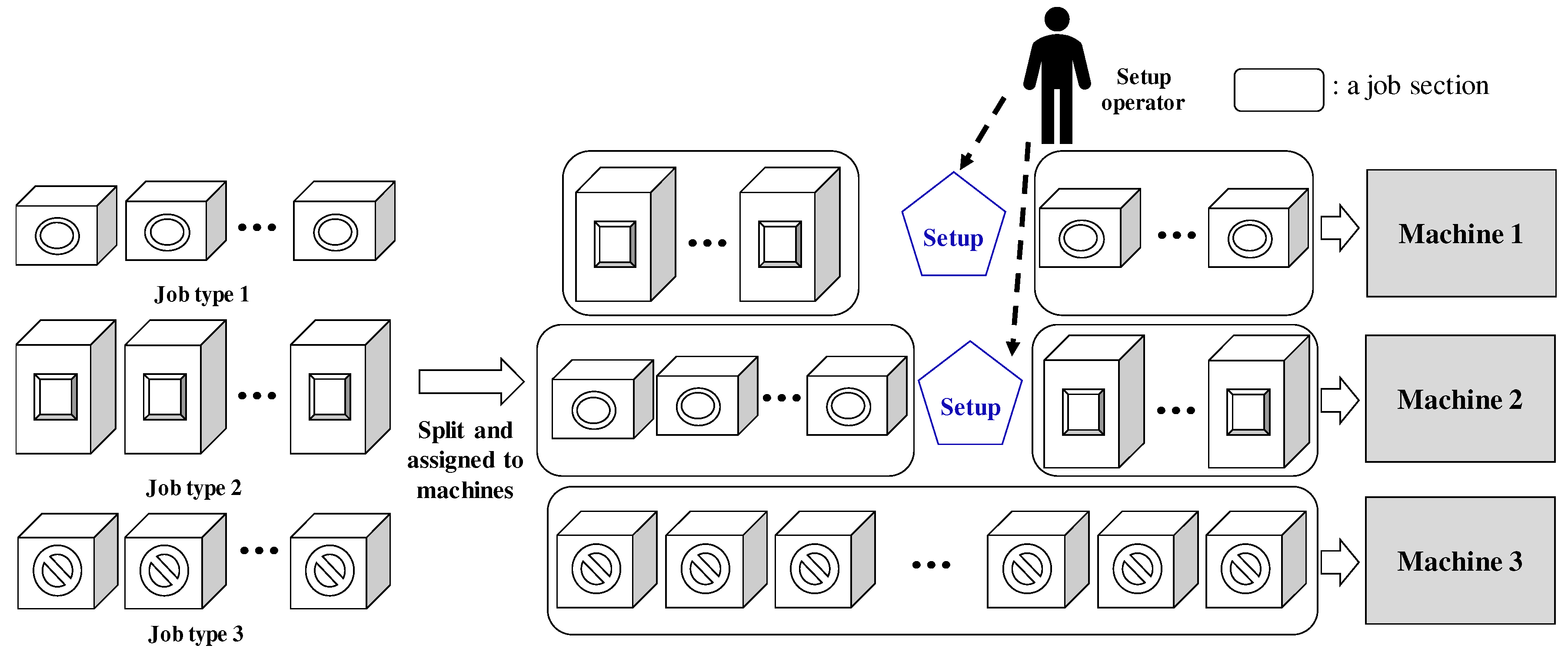
Figure 1 illustrates a simplified example in FFU manufacturing. In the example, there are three job types; many FFUs of Types 1–3 (see the left part of Figure 1). Jobs of each job type can be slit into multiple job sections, and they are assigned to machines. In this example, jobs of Types 1 and 2 can be processed on Machines 1 and 2, and jobs of Type 3 can only be processed on Machine 3 due to the dedicated machine constraint. In each machine, when job types change, a setup is required and it is performed by a human operator, as shown in Figure 1. In the example, there is only one human operator for setups and at most two setups can be required at the same time. In that case, one of two setups should be delayed, which makes the scheduling problem complicated.

Another factory we introduce is producing automotive pistons for Hyundai Motor Group, BMW, GM, and so on. Automotive pistons are first cast from aluminum alloys in uniform parallel machines, and then go through machining and assembly process steps. The multiple parallel machines for casting processes are classified into automatic, semi-automatic, and manual machines, and each of them can handle a set of certain piston types because machines are equipped with different tools and some pistons have specific process requirements. In addition, high quality pistons should be tracked in each unit so that all process parameters for each unit are checked. In this case, pistons for those customers should be processed on the machines that have the tracking system, which introduces dedicated-machine constraints. A piston type consists of thousands of units so that they can be divided into several lots, and multiple piston types are produced at the same time. Setups when product types change are performed by an operator, and the setup times do not depend on the preceding product type.

As introduced, the problem considered in this paper has many real applications and is constrained by various scheduling requirements such as parallel machines with different speeds, dedicated machines, and limited setup operators. To the best of our knowledge, no study has considered this problem. Therefore, this paper is intended to contribute to this end by presenting a mathematical optimization model and developing efficient heuristic algorithms.

2. Literature Review

In this section, we review papers related to our problem. Since a uniform parallel machine scheduling problem with dedicated machines, job splitting, and setup resources is considered, relevant literature can be classified into three groups: studies considering parallel machines, job splitting, and resources.

First, there have been numerous papers on scheduling identical parallel machines. Many early studies have analyzed list schedules and the longest processing time (LPT) first rule with the makespan minimization measure on either identical or uniform parallel machines [8,9,10,11,12,13]. The authors of [8,9] analyzed the worst-case bound of an arbitrary list schedule and the LPT rule on identical parallel machines. In the work by Garey and Graham [10], bounds of list schedules on identical parallel machines with a set of resources where each job requires specified units of each resource at all times during its execution were provided. In the paper by Gonzalez et al. [11], the performance of the LPT schedules on uniform parallel machines was analyzed, and the study by Friesen [12] provided tighter bounds for the same problem. The work by Cho and Sahni [13] analyzed the worst-case bound of list schedules for uniform parallel machine scheduling problems. All of them assumed the nonpreemptive schedules for minimizing the makespan. From these papers, we can have insights to develop priority rules for heuristic algorithms presented in this paper.

For uniform parallel machine scheduling, the work by Dessouky et al. [14] developed many efficient algorithms with scheduling criteria that are nondecreasing in the job completion times, such as makespan, total completion time, maximum lateness, and total tardiness. The study by Dessouky [15] proposed a branch and bound algorithm for uniform parallel machine scheduling with ready times in order to minimize the maximum lateness. The work by Balakrishnan et al. [16] examined uniform parallel machine scheduling problems with sequence-dependent setup times in order to minimize the sum of earliness and tardiness costs. They provided a mixed integer formulation that has substantially small 0-1 variables for small-sized problems. In the study by Lee et al. [17], two heuristic algorithms for uniform parallel machine scheduling were developed to derive an optimal assignment of operators to machines with learning effects in order to minimize the makespan. The work by Elvikis et al. [18] also considered a uniform parallel machine scheduling problem with two jobs that consist of multiple operations, and derived Pareto optima with makespan and cost functions. In the study by Elvikis and T’kindt [19], the problem with multiple objectives related with the job completion times was investigated by developing a minimal complete Pareto set enumeration algorithm. The work by Zhou et al. [20] considered a batch processing problem on uniform parallel machines with arbitrary job sizes in order to minimize the makespan. They developed a mixed integer programming model and an effective differential evolution-based hybrid algorithm. In the work by Jiang et al. [21], a hybrid algorithm that combines particle swarm optimization and genetic algorithm was developed for scheduling uniform parallel machines with batch transportation. The study by Zeng et al. [22] examined a bi-objective scheduling problem on uniform parallel machines by considering electricity costs under time-dependent or time-of-use electricity tariffs. All of these studies are not directly applicable to our problem since we consider more complicated problem settings. However, some ideas and approaches used in this paper were inspired by these previous works.

One of the important features of our problem is job splitting. Some papers have considered the job splitting property on parallel machines. Several polynomial time algorithms for scheduling parallel identical, uniform, and unrelated machines with job splitting were developed in order to minimize maximum weighted tardiness [23]. In the work by Yalaoui and Chu [6], an efficient heuristic algorithm for parallel machine scheduling with job splitting and sequence-dependent setup times was proposed and its performance was evaluated. They transformed the problem into a traveling salesman problem and solved with Little’s method. It was further analyzed with a linear programming approach [24]. Kim et al. [7] developed a two-phase heuristic algorithm for parallel machine scheduling with job splitting where an initial sequence is constructed by an existing heuristic method for parallel machine scheduling in the first phase and then the jobs are rescheduled by considering job splitting in the second phase. Shim and Kim [25] further analyzed the same problem by developing a branch and bound algorithm with several dominance properties. In the study by Park et al. [26], heuristic algorithms for minimizing total tardiness of jobs on parallel machines with job splitting were presented. Wang et al. [27] also examined a parallel machine scheduling problem with job splitting and learning with the total completion time measure, and used a branch and bound algorithm for small-sized problems and heuristics for large-sized ones. Even though most of these previous studies considering job splitting assume simpler manufacturing environment than that of our problem, they provide an idea of algorithm design for the heuristics developed in this paper.

Lastly, many papers have also considered resources in scheduling parallel machines, which is an important scheduling requirement of our problem. In the work by Kellerer and Strusevich [28], a parallel dedicated machine scheduling problem with a single resource for the makespan minimization was examined. They analyzed the complexity of different variants of the problem and developed heuristic algorithms employing the group technology approach. Kellerer and Strusevich [29] further considered the problem with multiple resources, and developed polynomial-time algorithms for special cases. In the study by Yeh et al. [30], several metaheuristic algorithms for uniform parallel machine scheduling were developed given that resource consumption cannot exceed a certain level. These studies assumed that resources are required to process jobs on machines. For setup resource constraints, the study by Hall et al. [31] dealt with nonpreemptive scheduling of a given set of jobs on several identical parallel machines with a common server was considered. In detail, they considered many classical scheduling objectives in this environment and proposed polynomial or pseudo-polynomial time algorithms for each problem considered. The work by Huang et al. [32] addressed a parallel dedicated machine scheduling problem with sequence-dependent setup times and a single server. Several papers have examined two-parallel machine scheduling problems with a server and proposed efficient heuristic algorithms [33,34,35]. The study by Cheng et al. [36] considered a common server and job preemption in parallel machine scheduling with the makespan measure and provided a pseudo-polynomial time algorithm for two machine cases and analyzed the performance ratios of some natural heuristic algorithms. Hamzadayi and Yildiz [37] also considered the same problem with sequence-dependent setup times and derived metaheuristic methods to minimize the makespan. For multiple servers, the study by Ou et al. [38] examined a parallel machine scheduling problem where servers perform unloading tasks of jobs and proposed a branch and bound and heuristic algorithms. Unlike the problem in this paper, most of studies considering resources in scheduling parallel machines assume a single resource (or server) or do not take into account other scheduling requirements considered in this paper such as job splitting and dedicated machines. Therefore, methods developed in the previous papers cannot be applied to our problem. For interested readers, reviews on parallel machine scheduling can be found in [39,40,41].

In summary, even though there have been numerous papers on parallel machine scheduling, no study has been performed for our problem; uniform parallel machine scheduling with dedicated machines, job splitting, and setup resource constraints. As explained above, this problem is motivated from real-world systems, and there are many other applications in which the proposed approach can be useful. We first describe the problem in detail and develop a mathematical programming model for the first time. We then provide four lower bounds and propose efficient heuristic algorithms. The performance of the algorithms is evaluated by comparing with lower bounds. An application of our algorithm to a real problem from industry is also introduced.

3. Problem Description & Analysis

In this study, we consider a uniform parallel machine scheduling problem with dedicated machines, job splitting properties, and limited setup resources, which can be easily observed in practice. In uniform parallel machine scheduling, n jobs are processed on m machines in parallel, but machines can have different speeds. The processing speed of machine i where $i\in M$, $M=\{1,2,..,m\}$, is denoted by $v_i$, which can be regarded as relative speeds. For example, if $v_1=2\times v_2$, Machine 1 is twice as fast as Machine 2. Job j, $j\in N$, $N=\{1,2,...,n\}$, has the processing time of $p_j$ if the machine speed is 1. Therefore, in general, the processing time of job j on machine i is $\frac{p_j}{v_i}$. When all machines have the same speed, e.g., $v_i=1$ for all i, the environment is the same as identical parallel machine scheduling which is a special case of our problem. Dedicated machines enforce that job j can only be processed on a set of designated machines, denoted as $M_j$, and can be split into multiple sections that can be processed on several machines simultaneously. When a job type is changed in a machine, a setup is needed by one of r ($<m$) operators that are generally insufficient to set up all of m machines at the same time (see Figure 1). The setup time for job j, $s_j$, is sequence-independent; that is, the setup time is not affected by the preceding job, and it only depends on the job to be processed. The objective is to minimize the maximum of machine completion times, $C_{max}$ where $C_{max}={max}_i{C}_i$ and $C_i$ indicates the completion time of machine i.

The problem considered in this paper can be easily proven to be NP-hard because parallel machine scheduling problems with two machines, which are a special case of our problem with $v_i=1$ for all $i\in M$, $r=m$, $s_j=0$ for all $j\in N$, and $M_j=M$ for all $j\in N$, are proven to be NP-hard [42]. We assume that jobs processed on machines for the first time do not require setup operations. This is because once all jobs are completed for a given period, mostly one or several weeks, preventive maintenance for machines is performed and then they are set up for the next desired states [6]. Setup times are not affected by different speeds of machines since they are performed by setup operators. The lengths of jobs processed on each machine and their sequence should be determined by considering setup resources and dedicated machines with different speeds in order to minimize the makespan. For a better understanding, we provide the following example.

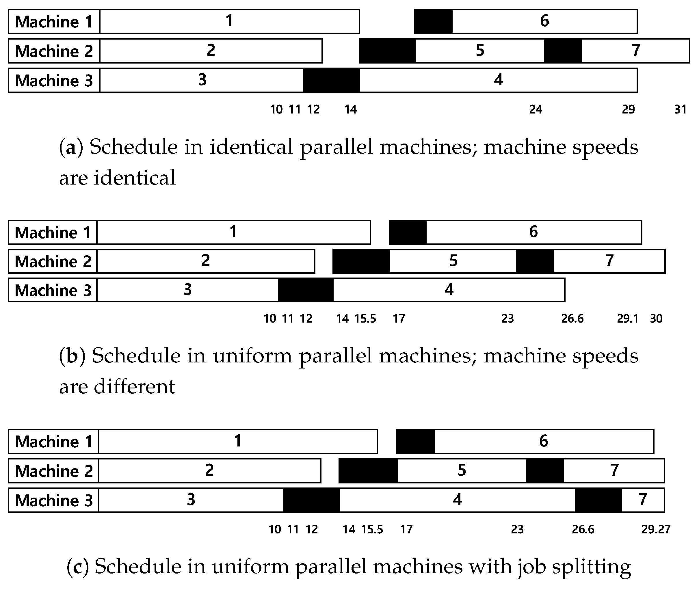
Example 1.

Suppose that there are three machines and seven jobs where $(p_j,s_j)$ for all j where $1\le j\le 7$ are given as $(14,5),(12,4),(11,4),(15,3),(7,3),(10,2),(5,2)$. Figure 2 shows three Gantt charts for production schedules in identical or uniform parallel machines with one setup operator. In the Gantt chart, numbers in white bars indicate job indices, and black bars represent setup operations. Numbers in the bottom denote time stamps; for example, in Figure 2a, Machine 2 finishes at 31 while completion time of Machines 1 and 3 is 29. Assume that jobs are processed in their index order, the jobs processed for the first time on each machine do not require setups, and there is no dedicated machine constraint. When jobs are processed on identical parallel machines, their makespan is 31, as illustrated in Figure 2a. However, when the machines have different speeds, i.e., $v_1,v_2$, and $v_3$ are 0.9, 1, and 1.1, respectively, the schedule becomes the same as the Gantt chart in Figure 2b, and the makespan is 30. In this case, the schedule can be improved by splitting Job 7 into two sections and assigning one section with the processing time of 0.73 to Machine 3. Since $v_3$ is 1.1, it takes 0.66 for the section to be completed on Machine 3 and the makespan becomes 29.27. If Job 7 can only be processed on Machines 1 and 2, i.e., $M_7=\{1,2\}$, splitting the job cannot improve the schedule. Hence, special considerations on scheduling uniform parallel machines with dedicated machines, job splitting, and setup resource constraints are required.

We now propose a mathematical programming model for uniform parallel machine scheduling with dedicated machines, job splitting, and setup resources for the first time.

Table 1. Symbols and descriptions for the mathematical programming model.

Symbol	Description
$C_{max}$	maximum completion time of machines
H	scheduling horizon; a given parameter
$x_{ijt}$	1 if a setup for job j starts on machine i at time t, and 0, otherwise
$y_{ij}$	1 if a section of job j is processed on machine i, and 0, otherwise
$L_{ij}$	length of a section of job j processed on machine i
$z_{ijk}$	1 if a section of job k is processed right after a section of job j on machine i, and 0, otherwise
$R_{ijt}$	1 if machine i is under the setup for a section of job j between t and $t+1$, and 0, otherwise
$p_j$	processing time of job j when the machine speed is 1
$v_i$	relative processing speed of machine i
$s_j$	setup time for job j; sequence-independent
N	set of jobs; $\left\{1,\cdots ,n\right\}$
$M_j$	set of machines that can process job j
$J_i$	set of jobs that can be processed on machine i

lists the symbols and their descriptions used in the following mathematical programming model. Especially, H indicates a given scheduling horizon which can be determined by $\frac{{\sum }_{j\in N}{p}_j}{{min}_{i\in M}{v}_i}+{\sum }_{j\in N}{s}_j$.

$$\mathrm{Minimize}{C}_{max}$$

(1)

$$\mathrm{Subject}\mathrm{to}\sum _{t=0}^H{x}_{ijt}\le 1,j\in N,i\in M_j$$

(2)

$$\sum _{i\in M_j}\sum _{t=0}^H{x}_{ijt}\ge 1,j=1,2,...,n$$

(3)

$$\sum _{t=0}^H{x}_{ijt}=y_{ij},j\in N,i\in M_j$$

(4)

$$\sum _{t=0}^{H}t{x}_{ijt}+(\frac{L_{ij}}{v_i}+s_j)y_{ij}+D(z_{ijk}-1)-z_{i0j}{s}_j\le \sum _{t=0}^{H}t{x}_{ikt}j\in N,i\in M_j,k\in J_i$$

(5)

$$C_{max}\ge \sum _{t=0}^{H}t{x}_{ijt}+(\frac{L_{ij}}{v_i}+s_j)y_{ij}-z_{i0j}{s}_j,j\in N,i\in M_j$$

(6)

$$\sum _{t=0}^H{x}_{ijt}=\sum _{k\in J_i\cup \{n+1\}}{z}_{ijk},j\in N,i\in M_j$$

(7)

$$\sum _{t=0}^H{x}_{ikt}=\sum _{j\in J_i\cup \left\{0\right\}}{z}_{ijk},k\in N,i\in M_k$$

(8)

$$\sum _{k\in J_i}{z}_{i0k}=1,i\in M$$

(9)

$$\sum _{j\in J_i}{z}_{i,j,n+1}=1,i\in M$$

(10)

$$z_{ijj}=0,j=1,2,...,n,i\in M_j$$

(11)

$$\sum _{i\in M_j}{L}_{ij}=p_j,j\in N$$

(12)

$$y_{ij}\le L_{ij},j=1,2,...,n,i\in M_j$$

(13)

$$y_{ij}\ge \frac{L_{ij}}{p_j},j\in N,i\in M_j$$

(14)

$$(x_{ijt}-z_{i0j})s_j\le \sum _{u=t}^{t+s_j-1}{R}_{iju},j\in N,i\in M_{j}t=0,1,...,H-\underset{j}{max}{s}_j$$

(15)

$$\sum _{t=0}^H{R}_{ijt}\le s_j\sum _{t=0}^H{x}_{ijt},j\in N,i\in M_j$$

(16)

$$\sum _{t=0}^H{R}_{ijt}\le s_j(1-z_{i0j}),j\in N,i\in M_j$$

(17)

$$\sum _{j=1}^n\sum _{i\in M_j}{R}_{ijt}\le r,t=0,1,...,H$$

(18)

$$x_{ijt},z_{ijk},y_{ij},R_{ijt}\in \{0,1\},L_{ij}\in {\mathbb{Z}}^{+}$$

(19)

The objective is to minimize $C_{max}$, which indicates the maximum completion time of machines. The constraint in Equation (2) is used for ensuring that a section of job j can be assigned to machine i, $i\in M_j$, only once; multiple assignments of sections of the same job type to a certain machine are not allowed. The constraint in Equation (3) is developed for job splitting property, which indicates that multiple sections of job j can be processed on different machines in $M_j$. The constraint in Equation (4) associates $x_{ijt}$ and $y_{ij}$ so that if a section of job j is assigned to machine i, $y_{ij}$ and the sum of $x_{ijt}$ for all t should be the same. In the constraint in Equation (5), when a section of job j starts to be processed on machine i, the next job k in $J_i$ should start after $t+\frac{L_{ij}}{v_i}+s_j$ time units where D is a large number. The term $z_{i0j}{s}_j$ is used to eliminate the setup time of the first job on machine i. The objective, $C_{max}$, is obtained with the constraint in Equation (6). Once a section of job j is processed on machine i, it should have its succeeding and preceding jobs as indicated by the constraints in Equations (7) and (8), respectively. The constraints in Equations (9) and (10) ensure that dummy jobs 0 and $n+1$ are the first and last jobs, respectively, on each machine. Since a section of job j cannot precede or success the same job type, $z_{ijj}=0$ as in the constraint in Equation (11). The sum of processing times for job j on machines in $M_j$ should be equal to $p_j$ from the constraint in Equation (12), and a section of job j is assigned to machine i, then $L_{ij}$ should be larger than 0 from the constraints in Equations (13) and (14). The constraints in Equations (15)–(18) are used for the setup resource constraints. If a section of job j starts to be processed on machine i at time u, $R_{ijt}$ should be 1 for all t where $u\le t\le u+s_j-1$, which is constrained by the constraints in Equations (15) and (16). The constraint in Equation (17) is used for the first jobs on machines because setup times for those jobs are ignored. Since there are r setup operators, the sum of $R_{ijt}$ at each time t should be less than or equal to r. Since $L_{ij}{y}_{ij}$ is nonlinear, we introduce $G_{ij}$, $G_{ij}=L_{ij}{y}_{ij}$, which indicates the length of a section of job j that is actually processed on machine i. Then, the commercial solvers such as CPLEX can be used to obtain optimal solutions with the proposed formulation. The following inequalities are added where D is a large number:

$$G_{ij}-L_{ij}\le D(1-y_{ij}),j\in N,i\in M_j$$

(20)

$$G_{ij}-L_{ij}\ge D(y_{ij}-1),j\in N,i\in M_j$$

(21)

$$G_{ij}\le D{y}_{ij},j\in N,i\in M_j$$

(22)

Optimal solutions from the mathematical formulation can be used to evaluate the performance of the proposed algorithm. However, large size problems cannot be solved within an acceptable time even with three machines and four jobs as our problem is NP-hard. Thus, lower bounds are derived and used for the performance evaluation. We define a job set $N_1$ as one that contains m jobs so that ${\sum }_{j\in N_1}{s}_j$ is maximized and those m jobs in $N_1$ can be assigned to m machines one by one while satisfying dedicated machine constraints. Suppose that there are two machines and three jobs, and $s_1$, $s_2$, and $s_3$ are 2, 1, and 3, respectively. If $M_1=M_3=\left\{1\right\}$ and $M_2=\{1,2\}$, $N_1$ contains Jobs 2 and 3 instead of Jobs 1 and 3 even though $s_2+s_3<s_1+s_3$ because Jobs 1 and 3 must be processed on Machine 1. A job set $N_2$ includes jobs that are in $N\backslash N_1$. We used the Hungarian method to obtain set $N_1$ with n jobs and n machines (m machines + ($n-m$) dummy machines) [43]. $S_l$ indicates a set of jobs that have the same set of dedicated machines, i.e., $M_j=M_k$ if jobs j and k are in $S_l$. In the above example, Jobs 1 and 3 are in the same set. We now present several lemmas to derive lower bounds.

Lemma 1.

A job-based lower bound $L{B}_1$ is ${max}_j\frac{p_j}{{\sum }_{i\in M_j}{v}_i}$.

Proof. 

Since job j can only be processed on machines in $M_j$, the minimum time required to complete job j is $\frac{p_j}{{\sum }_{i\in M_j}{v}_i}$. Hence, the maximum value among $\frac{p_j}{{\sum }_{i\in M_j}{v}_i}$ becomes a job-based lower bound. ☐

Lemma 2.

A machine-based lower bound $L{B}_2$ is $\frac{{\sum }_{j=1}^n{p}_j}{{\sum }_{i=1}^m{v}_i}+{\sum }_{j\in N_2}\frac{s_j}{m}$.

Proof. 

For a basic parallel machine scheduling problem, a lower bound is $\frac{{\sum }_{j=1}^n{p}_j}{m}$. In our problem, since m machines have different speeds, it takes at least $\frac{{\sum }_{j=1}^n{p}_j}{{\sum }_{i=1}^m{v}_i}$ to complete all of n jobs. In addition, the setup time of ${\sum }_{j\in N_2}{s}_j$ for $n-m$ jobs is required. Hence, a machine-based lower bound is $\frac{{\sum }_{j=1}^n{p}_j}{{\sum }_{i=1}^m{v}_i}+{\sum }_{j\in N_2}\frac{s_j}{m}$. ☐

Lemma 3.

A resource-based lower bound $L{B}_3$ is $\frac{{\sum }_{j\in N_2}{s}_j}{r}$.

Proof. 

Except the first m jobs assigned, $n-m$ jobs require setups that take at least ${\sum }_{j\in N_2}{s}_j$ as we defined previously. Since those setups are performed by r operators, a resource-based lower bound is $\frac{{\sum }_{j\in N_2}{s}_j}{r}$. ☐

Lemma 4.

A job set-based lower bound $L{B}_4$ is ${max}_{S_l}\{\frac{{\sum }_{j\in S_l}{p}_j}{{\sum }_{i\in M_{S_l}}{v}_i}+{\sum }_{j\in S_l^{\prime }}\frac{s_j}{|M_{S_l}|}\}$ where $M_{S_l}$ is a set of machines that can process jobs in $S_l$, and $S_l^{\prime }$ is a set of jobs in $S_l$ that does not contain $|M_{S_l}|$ jobs with the largest setup times among jobs in $S_l$.

Proof. 

For each job set, $S_l$, a lower bound can be obtained similarly as $L{B}_2$ in Lemma 2. Jobs in $S_l$ can only be processed on machines in $M_{S_l}$, which takes at least $\frac{{\sum }_{j\in S_l}{p}_j}{{\sum }_{i\in M_{S_l}}{v}_i}$. The setups for $|S_l|$ jobs require at least as much as ${\sum }_{j\in S_l^{\prime }}{s}_j$ since $|M_{S_l}|$ jobs can start at first on $|M_{S_l}|$ machines. Hence, the maximum value among $\frac{{\sum }_{j\in S_l}{p}_j}{{\sum }_{i\in M_{S_l}}{v}_i}+{\sum }_{j\in S_l^{\prime }}\frac{s_j}{|M_{S_l}|}$ for all $S_l$ becomes a job set-based lower bound. ☐

Corollary 1.

A lower bound of the makespan of the problem, $LB$, is $max\{L{B}_1,L{B}_2,L{B}_3,L{B}_4\}$.

4. Heuristic Algorithms

Since no setup is required for the first jobs on machines, assigning jobs with large setup times as the first ones can lead to the makespan reduction. However, sorting jobs in order of nonincreasing setup times and assigning the first m jobs to m machines may not be feasible or may lead to less setup time reductions due to the dedicated machines. Hence, we assign m jobs in $N_1$ to m machines so that the sum of setup times of those jobs is maximized. As mentioned above, the optimal assignment of m jobs to m machines can be found with the Hungarian method. In the method, $n-m$ dummy machines are made and setup times of n jobs on those machines are set to 0. The setup time of job j on machine i, $i\notin M_j$, is also set to 0. Then, the Hungarian method is applied with n jobs and n machines. It is known that the complexity of the Hungarian method is $O(n^3)$. With this method, we can maximize the sum of setup times of jobs that are first assigned to each machine.

After assigning m jobs, each time machines become available, jobs are chosen according to some of well-known priority rules. The first one is the least flexible job (LFJ) first rule. When machine i finishes processing a job, the job with the smallest $|M_j|$ among jobs in $J_i$ is chosen and assigned. The LFJ performs well for dedicated parallel machine scheduling. The second one is the LPT rule that selects the job with the largest processing time among jobs in $J_i$. After assigning all of n jobs, the loads of machines are balanced by splitting last jobs on each machine and assigning those sections to other machines by considering dedicated constraints and different speeds of machines.

We provide the procedures of the two priority rules for assigning $n-m$ jobs. Let $L_i$ as the earliest start time in which a job can be assigned to machine i by considering the setup resource constraints after assigning m jobs by the Hungarian method. The following rules are only applied to jobs in $N_2$.

LFJ rule

-

Step 1: For machine l where $l=arg{min}_{i\in M}{L}_i$, select job k in $J_l\bigcap N_2$ that has the smallest $|M_k|$ and assign the job to the machine. Ties are broken according to the LPT rule. Update $L_l$ to $L_l+s_k+\frac{p_k}{v_l}$, $N_2$ to $N_2\backslash \left\{k\right\}$, and $J_i$ to $J_i\backslash \left\{k\right\}$ where $i\in M_k$.

-

Step 2: If $N_2=\varnothing$, terminate. Otherwise, update $L_i$ for all $i\in M$ and go to Step 1.

LPT rule

-

Step 1: For machine l where $l=arg{min}_{i\in M}{L}_i$, select job k in $J_l\bigcap N_2$ that has the longest $p_k$ and assign the job to the machine. Ties are broken according to the LFJ rule. Update $L_l$ to $L_l+s_k+\frac{p_k}{v_l}$, $N_2$ to $N_2\backslash \left\{k\right\}$, and $J_i$ to $J_i\backslash \left\{k\right\}$ where $i\in M_k$.

-

Step 2: If $N_2=\varnothing$, terminate. Otherwise, update $L_i$ for all $i\in M$ and go to Step 1.

It is worth noting that another priority rule that combines the LPT and LFJ was also tested but provides a poor performance in the preliminary experiments; when a machine with a high speed becomes idle, a job is assigned according to the LPT rule, and, otherwise, the LFJ rule is applied to select a job.

We now propose a heuristic algorithm that combines the Hungarian method for assigning first m jobs, one of priority rules (LFJ or LPT) for assigning $n-m$ jobs and the load balancing step on machines. We tested the above two priority rules and show their performance in Section 5.

Algorithm 1: An iterative algorithm for uniform parallel machine scheduling

- Step 1: Using the Hungarian method, select m jobs and assign them to each machine so that the sum of setup times of such m jobs is maximized, and define a set $N_1$ that contains these first m jobs. - Step 2: Assign $n-m$ jobs in $N_2$ where $N_2=N\backslash N_1$ according to the LFJ or LPT rule. - Step 3: Select machine l where $l=arg{max}_{i\in M}{L}_i$. If maxReducibleTime(l)$>0$, assign a section of the last job on machine l to machine bestAssignableMachine(l) so that $L_l=L_{i^{*}}$ where $i^{*}=\mathbf{bestAssignableMachine}(\mathit{l})$, and repeat Step 3. Otherwise, go to Step 4. - Step 4: Consider $M_{k_l}$ where $l=arg{max}_{i\in M}{L}_i$ and $k_l$ is the last job on machine l. For each machine $i\in M_{k_l}$, update $L_i$ to $L_i-$maxReducibleTime(i) temporarily, and store its original value. If maxReducibleTime(l) $=0$, stop. Otherwise, let $j=$bestAssignableMachine(l) and restore $L_i$ to its original value. Assign a section of the last job on machine j to machine k where $k=$bestAssignableMachine(j) so that $L_j=L_k$, and go to Step 3.

Algorithm 2: Splitting jobs with long processing times to further improve solutions

- Step 1: Let both N and $N^{*}$ be the initial job list and $C_{max}=\infty$. - Step 2: Apply Algorithm 1 with jobs in N and update $C_{max}$ to the resulting makespan. If $C_{max}$ is equal to the lower bound, stop. Otherwise, go to Step 3. - Step 3: If $N^{*}=\varnothing$ or all of the jobs in $N^{*}$ have the processing time less than $ϵ$ ($ϵ$ is a very small positive real number to avoid an infinite loop), stop. Otherwise, select job l in $N^{*}$ according to the LPT rule. Split job l into two sections, $l_1$ and $l_2$, with the same processing time. Apply Algorithm 1 with jobs in $(N\backslash l)\cup \left\{l_1,l_2\right\}$. Let the makespan obtained with the updated N be $C_{max}^{{}^{\prime }}$. - Step 4: If $C_{max}^{{}^{\prime }}<C_{max}$, set $C_{max}=C_{max}^{{}^{\prime }}$ and update both N and $N^{*}$ by eliminating job l and adding jobs $l_1$ and $l_2$. Otherwise, update $N^{*}$ by eliminating l. Go to Step 3.

Function: maxReducibleTime($\mathit{l}$)

For a given machine l and its last job $k_l$, return $\Delta$ where $\Delta ={max}_{i\in M_{k_l}}\left[max\left\{\frac{L_l-L_i-d_{i,k_l}-s_{k_l}}{1+\frac{v_l}{v_i}},0\right\}\right]$.

Function: bestAssignableMachine($\mathit{l}$)

For a given machine l and its last job $k_l$, return machine i where $i=arg{max}_{i\in M_{k_l}}\left[\frac{L_l-L_i-d_{i,k_l}-s_{k_l}}{1+\frac{v_l}{v_i}}\right]$.

Assign m jobs with the Hungarian method and $n-m$ jobs with one of the priority rules in Steps 1 and 2, respectively. Then, the schedule is updated by balancing the loads of machines in Steps 3 and 4. In Step 3, the machine with the largest $L_i$ which currently determines the makespan is chosen, and for all other machines compute maximum reducible times by splitting and reassigning the last job of the machine with the largest $L_i$ to another machine. This step is repeated until there is no further improvement in makespan. Step 4 is specially designed to improve the solution under dedicated machine constraints. 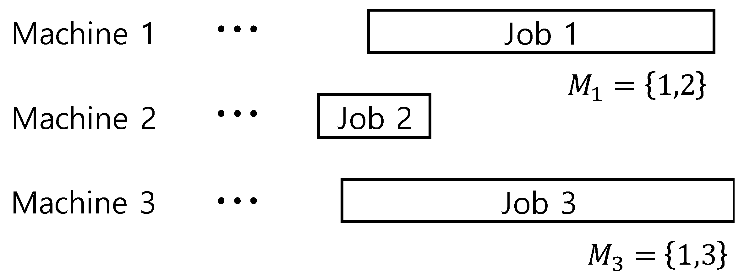Figure 3 shows an example where Step 4 of Algorithm 1 is effective. In Figure 3, Machine 3 has the longest completion time and the last job of Machine 3 is Job 3. In Step 3 of Algorithm 1, it is virtually impossible to have any improvement in makespan because Job 3 can be processed in Machines 1 and 3, but completion time of Machine 1 is almost the same as that of Machine 3. However, if the last job of Machine 1, Job 1, is split and reassigned to Machine 2 since $M_1=\left\{1,2\right\}$, the completion time of Machine 1 is decreased and thus we can have an additional chance to reduce the makespan. Based on this idea, Step 4 of Algorithm 1 is designed.

With Algorithm 1, we can obtain a feasible and acceptable solution. The solution is updated further by splitting jobs with long processing times at a time in Algorithm 2.

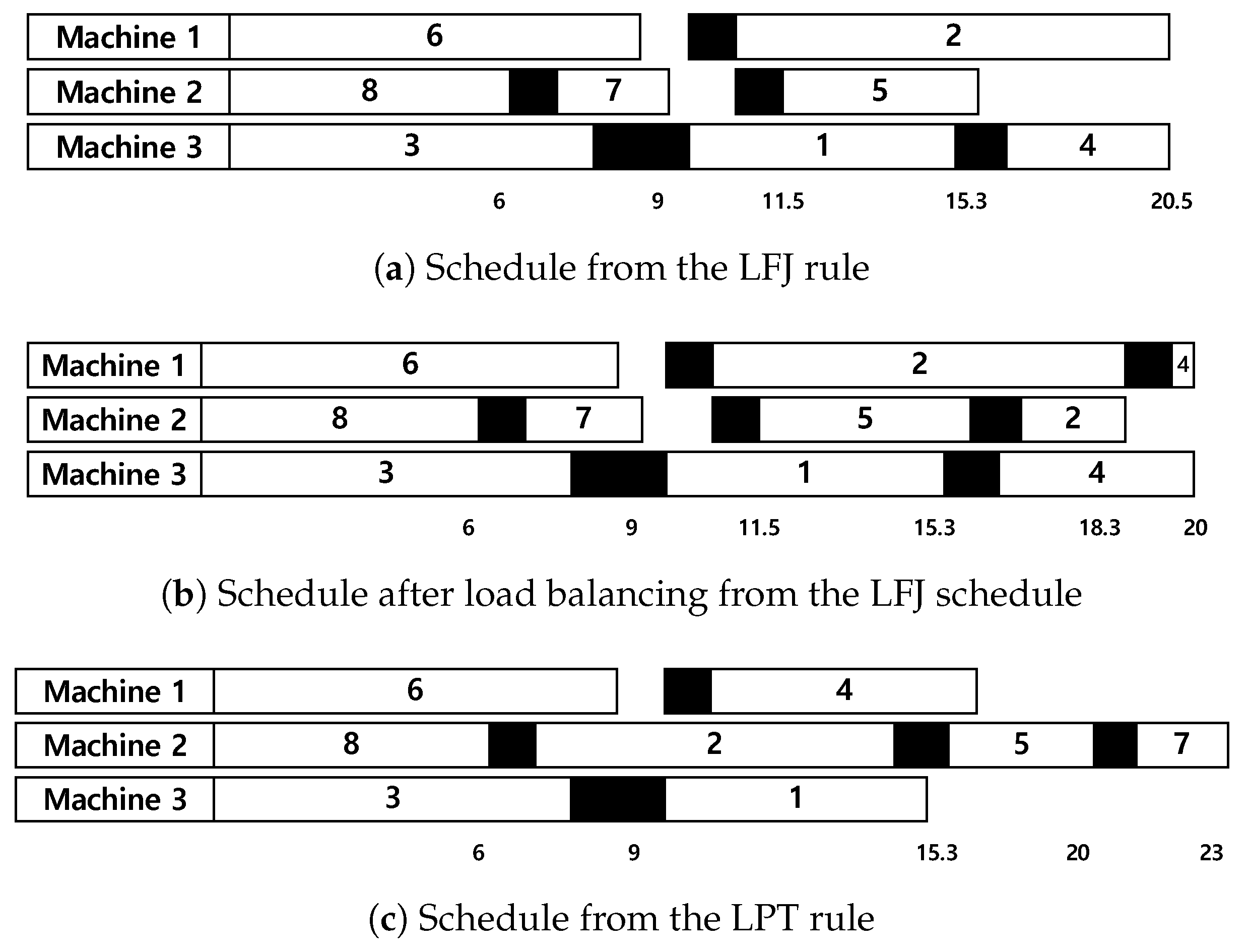
Example 2.

Suppose that there are three machines and eight jobs in which $v_1$, $v_2,$ and $v_3$ are 0.8, 1.0, and 1.2, respectively, and $(p_j,s_j)=(7,2),(8,1),(9,4),(5,1),(4,1),(7,4),(2,1),(6,3)$ for $1\le j\le 8$. Assume that $J_1=\{1,2,3,4,6,8\}$, $J_2=\{2,5,7,8\},$ and $J_3=\{1,3,4,5\}$. Figure 4a,c shows Gantt charts of schedules obtained from the LFJ and LPT rules, respectively, with r of 1. In Algorithm 1, the Hungarian method is first applied, and Jobs 6, 8, and 3 are assigned as the first jobs to Machines 1–3, respectively. Then, Machine 2 becomes idle at 6 time units, and Job 7 is selected since $|M_7|$ is the smallest one among jobs in $J_2$ according to the LFJ rule. After that, Machines 3 chooses Job 1 because all jobs in $J_3$ have the same value of $|M_j|$ where $j\in J_3$ and $p_1$ is the largest one. In a similar way, a complete schedule from the LFJ is obtained and its makespan is 20.5, as illustrated in Figure 4a. When the LPT rule is applied, Job 2 is first selected after Job 8 on Machine 2, and then Jobs 1 and 4 are assigned to Machines 3 and 1, respectively. The makespan is 23 since $|M_j|$ is not considered in the LPT rule. In Figure 4a, the last job, Job 4, on Machine 3 cannot be processed on Machine 2, and splitting the job into two sections and assigning one section to Machine 1 cannot improve the makespan. Hence, Job 2 on Machine 1 is split into two sections, and one is assigned to Machine 2. The schedule is further updated by splitting Job 4 on Machine 3 and assigning one section to Machine 1, as illustrated in Figure 4b. In this schedule, the makespan is 20. The schedules from the LPT rule cannot be improved by splitting the last jobs on machines. After maintaining the schedule, Algorithm 2 is applied.

5. Experimental Results

The proposed algorithms were tested with various scenarios. The machine speed was determined randomly between 0.8 and 1.2, and the setup times for jobs were generated with $\alpha p_j$ where $\alpha$ was selected randomly within $[0.01,0.1],[0.1,0.2],$ and $[0.1,0.5]$. Processing times were generated between 10 and 100. There were three levels of machine dedications, namely high, medium (i.e., mid), and low, and, in each level, jobs could be processed on a machine with the probability of 50%, 50–90%, and 90%, respectively. The scenarios had 5, 10, and 20 machines, each of which had 40, 60, and 80 jobs, respectively. The four algorithms, Algorithm 1 with LFJ (A1 (LFJ)), Algorithm 1 with LPT (A1 (LPT)), Algorithm 2 with LFJ (A2 (LFJ)), and Algorithm 2 with LPT (A2 (LPT)), were compared with lower bounds from Corollary 1. Average gaps were computed as follows:

$$\frac{\mathrm{makespan}\mathrm{from}\mathrm{the}\mathrm{proposed}\mathrm{algorithm}-\mathrm{lower}\mathrm{bound}}{\mathrm{lower}\mathrm{bound}}\times 100(\%).$$

(23)

For each problem with a certain range of setup times, a dedication level, and the specific number of resources, 100 instances were generated, and the average gaps are shown. Note that the mathematical formulation model can only solve small instances with two machines and four jobs to optimality within 1 h. We do not think it is meaningful to compare with such very small-sized instances, and furthermore for such cases gaps between makespans from our algorithm and lower bounds are extremely small.

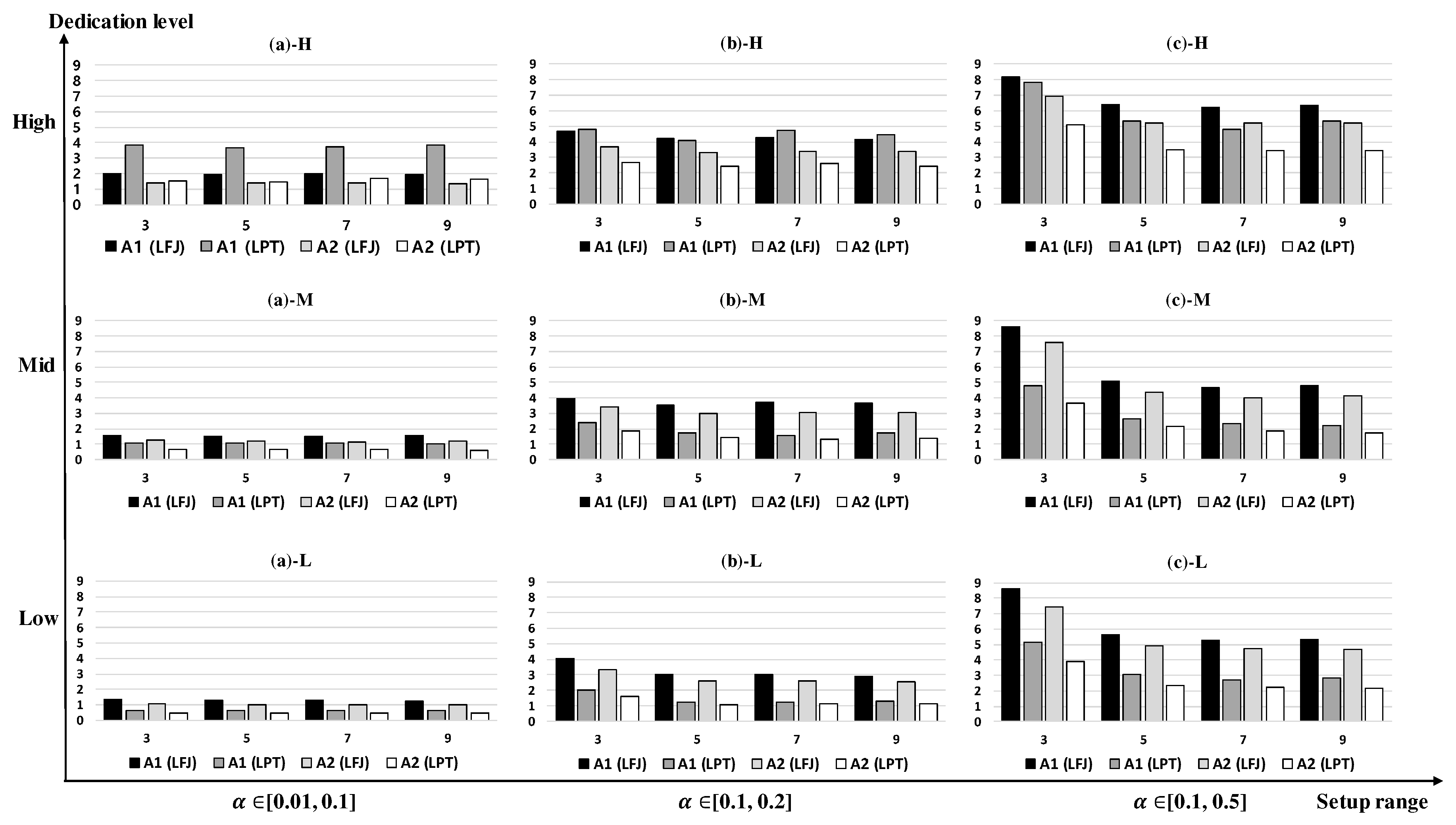
Figure 5, Figure 6 and Figure 7 show the experimental results with m of 10 and n of 40, 60, and 80, respectively. Each figure has nine graphs for the different setup time ranges and dedication levels. The graphs in those figures are labeled with (a), (b), (c) and H, M, and L according to setup ranges $\alpha \in [0.01,0.1]$, $\in [0.1,0.2]$, and $\in [0.1,0.5]$, and the dedication levels, respectively. For example, Figure 5a-H indicates the result with $\alpha \in [0.01,0.1]$ and the high dedication level. The number of servers, r, was set to be less than $\frac{m}{2}$ to reflect the resource constraints in the schedule. Each graph shows the average gaps of the four algorithms with r of 3, 5, 7, and 9. In Figure 5, the average gaps tend to increase as the setup time range is larger and the dedication level becomes high. In addition, as r becomes large, the gaps become smaller. A1 (LFJ) performs better than A1 (LPT) in Figure 5a-H,b-H whereas the average gaps of A1 (LPT) are smaller in other cases because LFJ rule works well with the high dedication level. In the case of Figure 5c-H, A1 (LPT) is slightly better than A1 (LFJ) because the machine loads may be well-balanced with LPT rule under the large setup times. When the machine dedication level is mid or low, A1 (LPT) is always better than A1 (LFJ). The average gap of A1 (LPT) is decreased significantly in Figure 5c-M compared to Figure 5c-H. The difference between A1 (LFJ) and A1 (LPT) becomes large under mid and low dedication levels as the setup time ranges increase whereas the difference is small with the high dedication. A2 (LFJ) and A2 (LPT) have patterns similar to A1 (LFJ) and A1 (LPT) in Figure 5. It is interesting to note that the average gaps of A1 (LFJ) and A2 (LFJ) in Figure 5c-M,c-L are slightly larger than those in Figure 5c-H, respectively, when r is small, whereas the average gaps are mostly large when the dedication level is high. This may indicate that when setup times are large and resource constraints are tight, LFJ rule provides good solutions with the high dedication level. This feature can also be found in Figure 6 and Figure 7. A2 (LPT) provides the smallest gaps among the four algorithms for all cases except Figure 5a-H. A2 (LPT) has the largest average gap of 3.88% in Figure 5c-H, and the smallest average gap of 0.48% in Figure 5a-L.

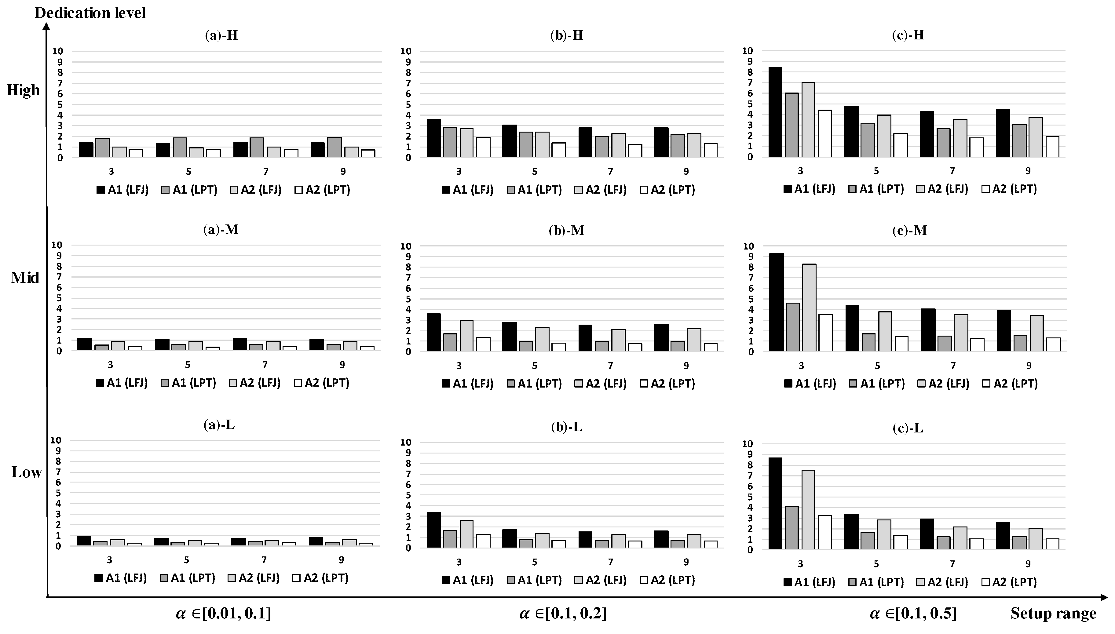
The nine graphs in Figure 6 have the features similar to those in Figure 5, but the average gaps are smaller as n increases. The large gaps are obtained when $\alpha \in [0.1,0.5]$ and r is small. A1 (LFJ) performs better than A1 (LPT) in Figure 6a-H but it is outperformed in all the other cases. A1 (LFJ) and A2 (LFJ) work poorly especially with large setup times and small resources compared to A1 (LPT) and A2 (LPT). A2 (LPT) performs well in most cases, and its largest and smallest average gaps are 2.57% and 0.29% in Figure 6c-H,b-L, respectively. 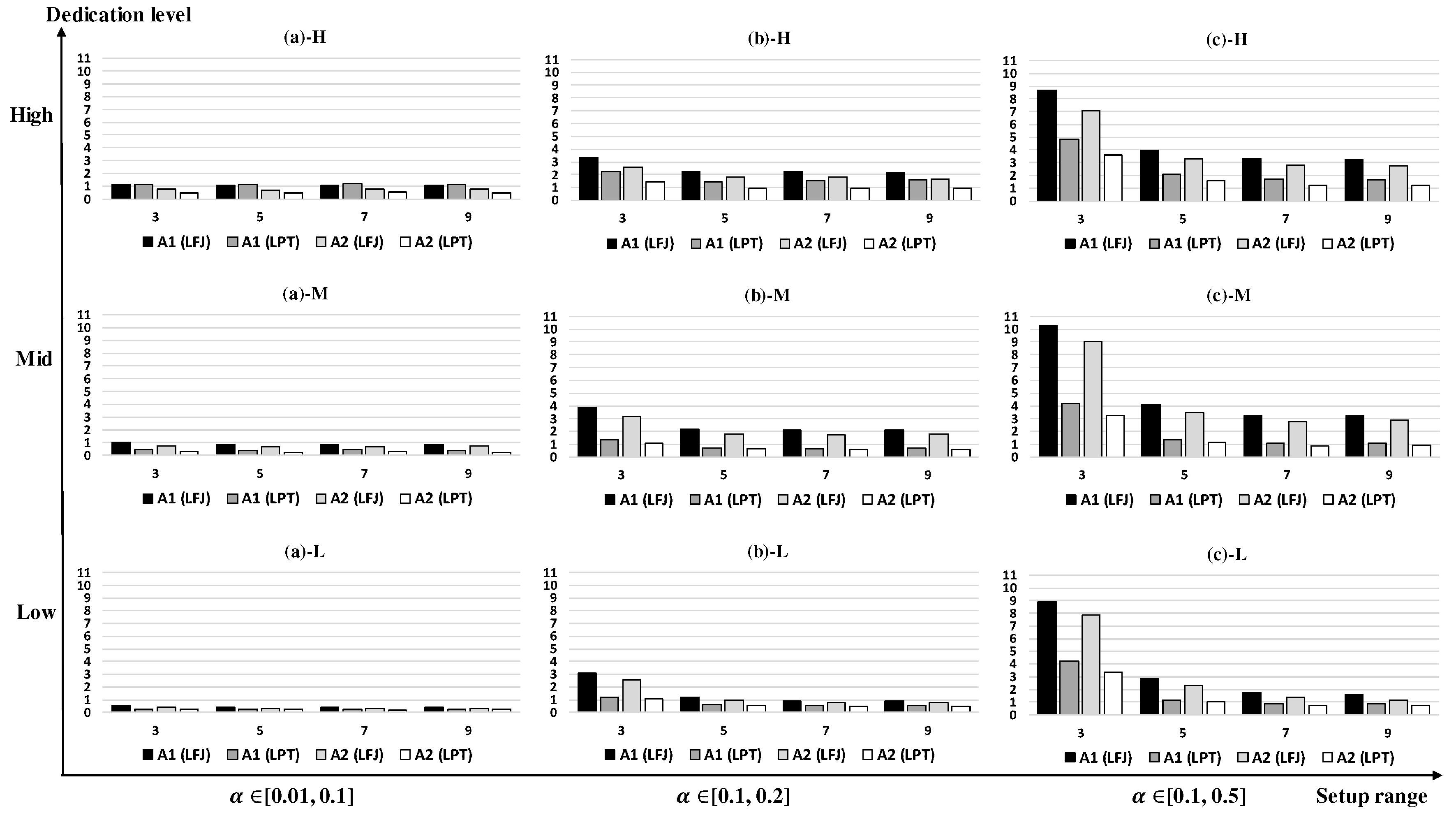Figure 7 shows the results with n of 80. We can see that A1 (LPT) performs better than A1 (LFJ) in Figure 7a-H unlike the previous results. The average gaps of the four algorithms are smaller than those in Figure 6 except for A1 (LFJ) with large setup times and small resources. This may indicate less tight lower bounds or poor performance of LFJ rule with large n. A2 (LPT) provides the largest and smallest average gaps that are 1.88% and 0.21% in Figure 7c-H and in Figure 7b-L, respectively. It is good to use A2 (LFJ) with small n, high machine dedication, and small setup times. Otherwise, A2 (LPT) is better.

Table 2. Summary of computational results with m of 10.

Instances		A1 (LFJ) (%)		A1 (LPT) (%)		A2 (LFJ) (%)		A2 (LPT) (%)
	Machine Speed	0.8–1.2	0.5–1.5	0.8–1.2	0.5–1.5	0.8–1.2	0.5–1.5	0.8–1.2	0.5–1.5
Dedication level	High	3.48	4.28	3.05	4.55	2.79	3.45	1.80	2.84
	Mid	3.28	3.86	1.52	2.30	2.80	3.29	1.17	1.90
	Low	2.58	3.24	1.25	2.00	2.16	2.71	1.02	1.74
Setup range	$\alpha \in [0.01,0.1]$	1.17	1.52	1.12	1.74	0.87	1.15	0.57	0.99
	$\alpha \in [0.1,0.2]$	2.87	3.63	1.74	2.77	2.35	3.03	1.21	2.08
	$\alpha \in [0.1,0.5]$	5.31	6.23	2.96	4.34	4.53	5.28	2.21	3.42
Resources	3	4.59	4.96	2.82	3.48	3.86	4.13	1.98	2.63
	5	2.77	3.48	1.70	2.87	2.28	2.88	1.17	2.05
	7	2.56	3.40	1.60	2.70	2.10	2.81	1.09	1.99
	9	2.54	3.33	1.64	2.75	2.10	2.77	1.08	1.97
No. of jobs	40	3.87	4.70	2.85	4.23	3.23	3.87	1.88	2.93
	60	2.94	3.58	1.71	2.56	2.42	2.97	1.20	1.94
	80	2.53	3.10	1.27	2.06	2.10	2.61	0.92	1.62

summarizes all of the results in Figure 5, Figure 6 and Figure 7 according to the different dedication levels, setup ranges, resources, and the number of jobs. Table 2 also shows the results with different machine speed ranges, 0.5–1.5. We can see that the average gaps tend to become smaller as the dedication level becomes lower, setup time ranges are smaller, the number of resources is larger, and the number of jobs becomes large. The average gaps of the four algorithms are 3.12%, 1.99%, 2.58%, and 1.33%, and hence we can obtain solutions close to optimal ones with A2 (LPT), respectively. The performances of A1 (LFJ) and A1 (LPT) are improved as much as 17% and 33% by using Algorithm 2, respectively. When the variation of machine speeds is larger, the average gaps also increase. Even if the machine speed is selected between 0.5 and 1.5, the average gaps are less than 5%. We note that the computation times of A1 (LFJ) and A1 (LPT) are less than 1 s, and it takes at most 61 s for A2 (LFJ) and A2 (LPT) with n of 80.

The detailed experimental results for m of 5 and 20 with n of 40, 60, and 80 are given in Appendix A.

Table 3. Summary of computational results with m of 5.

Instances		A1 (LFJ) (%)	A1 (LPT) (%)	A2 (LFJ) (%)	A2 (LPT) (%)
Dedication level	High	1.73	3.17	1.36	1.45
	Mid	1.40	1.20	1.12	0.73
	Low	0.85	0.71	0.70	0.59
Setup range	$\alpha \in [0.01,0.1]$	0.46	1.30	0.34	0.50
	$\alpha \in [0.1,0.2]$	1.18	1.54	0.95	0.83
	$\alpha \in [0.1,0.5]$	2.33	2.25	1.90	1.45
Resources	2	2.27	2.25	1.79	1.41
	3	1.17	1.60	0.94	0.82
	4	0.95	1.49	0.78	0.75
	5	0.91	1.44	0.74	0.71
No. of jobs	40	1.69	2.55	1.37	1.38
	60	1.24	1.45	0.98	0.78
	80	1.05	1.09	0.83	0.61

and

Table 4. Summary of computational results with m of 20.

Instances		A1 (LFJ) (%)	A1 (LPT) (%)	A2 (LFJ) (%)	A2 (LPT) (%)
Dedication level	High	5.14	3.85	4.29	2.76
	Mid	4.61	2.98	4.03	2.32
	Low	4.38	2.79	3.89	2.21
Setup range	$\alpha \in [0.01,0.1]$	2.05	1.55	1.61	1.02
	$\alpha \in [0.1,0.2]$	4.79	2.95	4.11	2.29
	$\alpha \in [0.1,0.5]$	7.30	5.13	6.49	3.98
Resources	7	4.86	3.38	4.20	2.54
	10	4.69	3.17	4.03	2.41
	13	4.65	3.16	4.02	2.38
	16	4.66	3.14	4.02	2.39
No. of jobs	40	5.94	5.32	5.11	4.01
	60	4.47	2.65	3.89	1.98
	80	3.72	1.66	3.21	1.30

show the summary of the results with m of 5 and 20, respectively, with the speed between 0.8 and 1.2. We can see the features similar to the results in Table 2. When m is 5, A1 (LFJ) and A2 (LFJ) have the largest average gaps when the number of resources is small, whereas A1 (LPT) and A2 (LPT) perform poorly when the dedication level is high. On the other hand, A1 (LFJ) and A2 (LFJ) provide the largest average gaps when the number of jobs is small as m increases. When m is 20, the average gaps of A1 (LPT) and A2 (LPT) are also large with n of 40 compared to other scenarios. By comparing the results in Table 2, Table 3 and Table 4, we can see that the average gaps tend to increase as m increases. The average gaps of the four algorithms with m of 5 and 20 are 1.33%, 1.70%, 1.06%, and 0.92%, and 4.71%, 3.21%, 4.07%, and 2.43%, respectively. The gaps are not large by considering the fact that they are computed with lower bounds not the optimal ones. The performance of Algorithm 1 is improved significantly by applying Algorithm 2. We can conclude that practical problems can be solved efficiently especially with A2 (LPT). The computation time for the scenarios with m of 20 and n of 60 is 89.43 s on average, and the maximum computation time is 100.17 s.

We further evaluated the four algorithms with extreme cases in which the number of resources is about 20% of the number of machines. In practice, r was set to be larger than 50% of m to increase the efficiency of the system. For each of setup time ranges, dedication levels, and the number of jobs, 100 instances were generated.

Table 5. Computation results of extreme cases.

Instances	n	A1 (LFJ) (%)	A1 (LPT) (%)	A2 (LFJ) (%)	A2 (LPT) (%)
	40	9.96	8.75	8.67	7.13
$m=5,r=1$	60	9.66	7.86	8.45	6.77
	80	9.02	7.23	7.81	6.29
	40	8.49	6.34	7.38	4.54
$m=10,r=2$	60	9.46	5.84	8.35	4.64
	80	10.20	5.86	9.08	4.89
	40	7.16	6.01	6.20	4.44
$m=20,r=4$	60	6.83	4.34	6.01	3.17
	80	7.47	4.48	6.60	3.25

shows the average gaps of the four algorithms with m of 5, 10, and 20. The large gaps are mostly obtained when $\alpha \in [0.1,0.5]$ and the dedication level is high. When m is 5, the gaps tend to decrease as n increases, whereas the gaps are large with the large number of jobs when m is 10, especially with A1 (LFJ) and A2 (LFJ). When m is 20, the instances with n of 60 provide the smallest gaps. We can see that, even in the extreme cases, A2 (LPT) provides the maximum average gaps of 7.13% when m and n are 5 and 40, respectively.

We finally tested our algorithms with a practical instance from an FFU factory in Korea. There were seven parallel machines in which three machines had the speed of 1.2 and the rest had the speed of 1. The setup times were not large, $\alpha \in [0.1,0.2]$. The number of jobs was 20, 30, and 40, each of which had processing times of 1–30, 1–20, or 1–10, respectively, to have a one-week production schedule. The number of setup operators was 2, and the dedication level was mid.

Table 6. Performance of the algorithm with a real application.

Instances	n	A1 (LFJ) (%)	A1 (LPT) (%)	A2 (LFJ) (%)	A2 (LPT) (%)
	20	6.40	5.35	6.02	3.68
$m=7,r=2,\alpha \in [0.1,0.2]$	30	5.01	4.24	3.91	2.61
	40	4.84	3.98	3.27	2.41

shows the results with m of 7 and n of 20, 30, and 40. We can see that the average gaps are less than 4% with the A2 (LPT). As shown in the table, A2 (LPT) provides very efficient solutions in this case.

6. Conclusions

We investigate a parallel machine scheduling problem for makespan minimization with various scheduling requirements such as different processing speeds of machines, dedicated machines, job splitting, and limited setup operators. We first present a mathematical model, which clearly describes our problem and can be used to obtain optimal solutions for small-sized problems. Since the problem considered is NP-hard, we develop an efficient heuristic algorithm for practical problems, which first obtains a feasible solution and then improves the solution in a constructive way. The performance of the algorithm was tested with various scenarios and a real problem from industry. Finally, we can conclude that the algorithm proposed is very efficient and provides highly acceptable solutions for most practical cases.

In future research, analytical results of the heuristic algorithm such as wort-case performance bounds need to be derived. In another direction, the problem can be extended to cover other scheduling requirements; for example, sequence-dependent setup times.