Renewable Energy Generation Assessment in Terms of Small-Signal Stability

Abstract

The popularity and role of renewable energy in the power grid are increasing nowadays as countries are shifting to cleaner forms of energy. This brings new challenges in maintaining a secure and stable power system, as renewable energy is known to be intermittent in nature and may introduce stability issues to the grid. In this paper, a screening framework of renewable energy generation scenarios is proposed to determine which power system conditions and scenarios will make the system unstable. The scenario screening framework is based on a sensitivity analysis of the system eigenvalues with respect to the renewable energy penetration to the system. The average scheduled renewable energy output, forecasting error standard deviation, average forecasting error, and bus location of the renewable energy source were used to define a renewable energy generation scenario. Depending on the amount and variability of renewable energy, there is a possibility for a critical eigenvalue to cross the imaginary axis. The estimated eigenvalue location resulting from the penetration of variable renewable energy is computed by adding the computed eigenvalue sensitivity to the initial operating point. If any of the estimated system eigenvalues cross the imaginary axis, the power system might be unstable in this scenario, so it requires more detailed simulations and countermeasures. Renewable energy forecasting was done using the long short-term memory model, and the proposed method was simulated using the IEEE 39-bus New England test system. The results of the proposed method were verified by comparing the simulation results to the eigenanalysis solution. The obtained results have shown that the proposed method can determine whether the renewable energy generation scenario is critical in power system operation.

1. Introduction

As the safe global warming limit has changed from 2 to 1.5$°$C above preindustrial levels [1], tightened policies and procedures from governments around the world are expected to be passed in order to eradicate CO₂ emissions and to shift fully to renewable energy (RE). Because of the heightened interest in integrating RE sources such as wind and solar energy in the power system, the need for integration studies of these renewable sources also increases. This is because of the intermittent nature that is associated with RE sources, a secure power system should be able to maintain stability, even with fluctuating RE output and be able to withstand the resulting contingencies or disruptions. Security assessment is done to determine if the power system can withstand disturbances without suffering a drop in the customer service level provided by the transmission and distribution companies [2]. Dynamic security assessment (DSA) is a type of security assessment that studies the security of the transient and dynamic responses to system disturbances in different timescales [3]. With the help of an online DSA [4,5], power system planners and operators can monitor the power system security in real-time, and they have the ability to act immediately in case of a critical disturbance occurring in the system. The transient energy function [6] and trajectory sensitivities [7] have both been used to analyze dynamic security assessments of the system. The difference between the two methods is that the analysis becomes more complex while using transient energy functions especially when dealing with big differential and algebraic equation (DAE) models of power systems [7]. The main features of an online DSA system include contingency screening, time simulations for stability assessment, calculation of power transfer limits, and concurrent processing of contingencies [4]. Contingency analysis is done on a single-base case scenario to determine how the system will react to any contingency event, which can be a planned or unplanned loss of a system element. The contingency screening function reduces the number of contingencies to be considered by the system operators by identifying the list of contingencies with a high likelihood of occurrence. Similarly, a scenario screening function identifies the base case scenarios that will be critical to the stability of the power system. There are different power system parameters in a base case scenario that can be analyzed, but for the purposes of this paper, scenarios will be limited to an analysis of RE generation scenarios.

Depending on the amount of RE generation forecasted for the next day, system operators will plan a day ahead which generators will be operated and at what generation output each generator is contracted to produce. During actual operations, the actual RE generation may differ from the forecasted RE output because of unforeseeable and uncontrollable external factors. The fluctuations in actual RE generation may result in a lower or higher total generated energy. This intermittency of RE can cause small disturbances to the power system because the power balance between the generated and distributed energy will not be equal. Small-signal stability refers to the ability of the power system to maintain synchronism when subjected to small disturbances [8].

In this paper, RE is considered as a small disturbance because the equations representing the power system can be linearized for the purpose of small-signal analysis [8]. In order to describe the small-signal stability of the power system for RE generation scenarios, eigenvalues of the power system must be analyzed. If an eigenvalue is found at the right-half of the complex plane, the system is unstable. Various methods were proposed to determine the trajectory of the eigenvalues as a system parameter is increased [9,10,11]. In [9], eigenvalue tracing is done by combining the invariant subspace method and the predictor–corrector scheme. An integration-based approach is used in [10] to trace critical eigenvalues and is combined with an index to determine which eigenvalues are considered critical. While in [11], the invariant subspace method is used with the projected Arnoldi method to trace the critical eigenvalues. The difference of trajectory tracing with the proposed method is that trajectory tracing involves a single parameter to be increased until a bifurcation occurs. This will not be applicable for scenario screening because each scenario is tested for its stability according to the small-signal stability rules. A more applicable approach is to determine the sensitivity of the eigenvalues. An eigenvalue sensitivity analysis was proposed in [12,13,14,15] to depict how the eigenvalues are affected by any change in the parameters of the power system. The method for determining the sensitivity of eigenvalues for sparse formulations of the power system equations has been presented in [12]. Eigenvalue sensitivity analyses, with respect to operating parameters [13] and power system parameters [14], have also been proposed in the literature. The augmented matrix using only dominant eigenvalues and their corresponding left and right eigenvectors were used in [15]. Lower-upper (LU) factorization, sparse matrices, and parallel computing techniques were used in computing the eigenvalue sensitivity of operating parameters [16]. Aside from power systems, the eigenvalue sensitivity was also used in parametric optimization. For instance, eigenvalue sensitivity was used to optimize the parameters of a doubly-fed induction generator (DFIG) wind turbine system [17,18]. Variation of different system parameters of microgrids with constant power loads was analyzed using eigenvalue sensitivity analysis in [19]. In the methods mentioned above, the screening of scenarios by analyzing the sensitivity of the eigenvalues with respect to the variation of RE has not been studied for power systems.

In daily operations, RE generation at each time period needs to be estimated based on day-ahead forecasting, so that operating points are established for security assessment. In the literature, several regression techniques have been adopted for RE forecasting. Autoregressive moving average (ARMA) and autoregressive integrated moving average (ARIMA) have become two of the most popular methods that can be used for linear time series analysis [20]. Aside from regression techniques, artificial intelligence (AI) techniques and hybrid methods were also proposed in the literature. For photovoltaic (PV) forecasting, the long short-term memory (LSTM) recurring neural network, which is a method under AI techniques, has become popular to implement because of its better performance compared to other conventional implementations [21]. This paper employs LSTM as the method for forecasting RE day-ahead generation because, aside from the historical PV output, historical cloud cover data are also utilized. Even though the accuracy of the forecasting techniques has improved over time, the actual generated output might still be different from the forecasted output because of the limitations of forecasting as well as unpredictable external sources affecting the generation of RE. Thus, for secure operation of the power system with RE resources, diverse RE generation scenarios need to be assessed in terms of several security issues. RE generation scenarios for examination are established for a specific time period using RE bus location, average forecasting error, forecasting error standard deviation, and average scheduled RE output. Depending on these factors, certain scenarios might be critical and result in insecure or unstable conditions. In order to keep the power system secure and stable under any circumstances, critical scenarios must be identified by power system planners to come up with countermeasures against the corresponding insecure phenomena.

This paper presents a framework for screening of RE generation scenarios in terms of small-signal stability, and it is based on eigenvalue sensitivity analyses with respect to RE generation. Eigenanalysis for the initial operating point is performed first, and sensitivities of critical eigenvalues with respect to RE variation are evaluated to estimate the movement of the eigenvalues and to check whether the resulting locations violate small-signal stability criteria. If some of the estimated eigenvalue locations are not in the acceptable region, the corresponding RE generation scenario is included in the critical scenario list and should be reassessed using a detailed stability analysis. The results of the proposed method were verified by comparing it with an eigenanalysis of the newly established operation with the corresponding RE generation scenario. Instead of performing an eigenanalysis for all possible operating points, the proposed screening framework can quickly determine whether each RE generation scenario might cause insecurity and instability. By implementing the proposed method in screening RE generation scenarios, only the critical scenarios need to be analyzed in depth by system operators for countermeasure determination. The contributions of this paper can be summarized as follows: (i) establishment of the framework to screen RE generation scenarios in terms of small-signal stability, (ii) inclusion of RE generation parameters such as average forecasting error, forecasting error standard deviation, and average scheduled RE output in the computation of the RE variability factor, (iii) application of eigenvalue sensitivity with respect to RE generation to determine small-signal stability, and (iv) formulation of the uncertainty of the real part of critical eigenvalues with respect to RE generation.

The paper is organized as follows: In Section 2, the mathematical background and the formulation of the system model, system state matrix and the eigenvalue sensitivity concept are presented. In Section 3, the proposed scenario screening framework based on the eigenvalue sensitivity analysis is presented. In Section 4, a day-ahead RE forecast is made using a LSTM model for RE generation scenarios. In the same section, the proposed method is applied to the New England Test System (IEEE-39 bus test system) to demonstrate its capability of determining the small-signal stability of the system for the five given scenarios. In Section 5, the conclusions of the study are presented.

2. Mathematical Background and System Formulation

This section presents the formulation and mathematical background of the system model, system state matrix, and the eigenvalue sensitivity concept used in this paper. The descriptions of the variables and parameters in the formulation of the system model are shown in

Table 1. Variables and parameters of the test system.

Variable/Parameter	Description
$\delta$	rotor angle [rad]
$\omega$	machine frequency [rad/s]
$E_q^{\prime }$	quadrature axis electromotive force (emf) [pu]
$E_d^{\prime }$	direct axis emf [pu]
${\omega }_{sys}$	system frequency [rad/s]
${\omega }_0$	system rated frequency [rad/s]
$P_m$	mechanical power generated by the prime mover [pu]
$D$	damping constant [pu]
$R_s$	armature resistance [pu]
$X_d$	direct axis synchronous reactance [pu]
$X_d^{\prime }$	direct axis transient reactance [pu]
$X_q$	quadrature axis synchronous reactance [pu]
$X_q^{\prime }$	quadrature axis transient reactance [pu]
$M$	inertia constant [pu]
$E_{fd}$	field winding voltage [pu]
$V_r$	automatic voltage regulator (AVR) output [pu]
$R_f$	exciter feedback [pu]
$T_{d0}$	time constant for the direct axis open circuit [s]
$T_{q0}$	time constant for the quadrature axis open circuit [s]
$T_e$	time constant for the exciter [s]
$T_a$	time constant for the AVR [s]
$T_f$	time constant for the feedback [s]
$K_e$	gain constant of the exciter [pu]
$K_a$	gain constant of the AVR [pu]
$K_f$	gain constant of the feedback [pu]
$V_{ref}$	reference voltage of the AVR [pu]
$P_m$	mechanical power output of the prime mover [pu]
$\mu$	generator steam valve opening [pu]
$T_{ch}$	time constant for the prime mover [s]
$T_g$	time constant for the speed governor [s]
$R$	droop constant [pu]
$P_{RE}$	RE generation [pu]

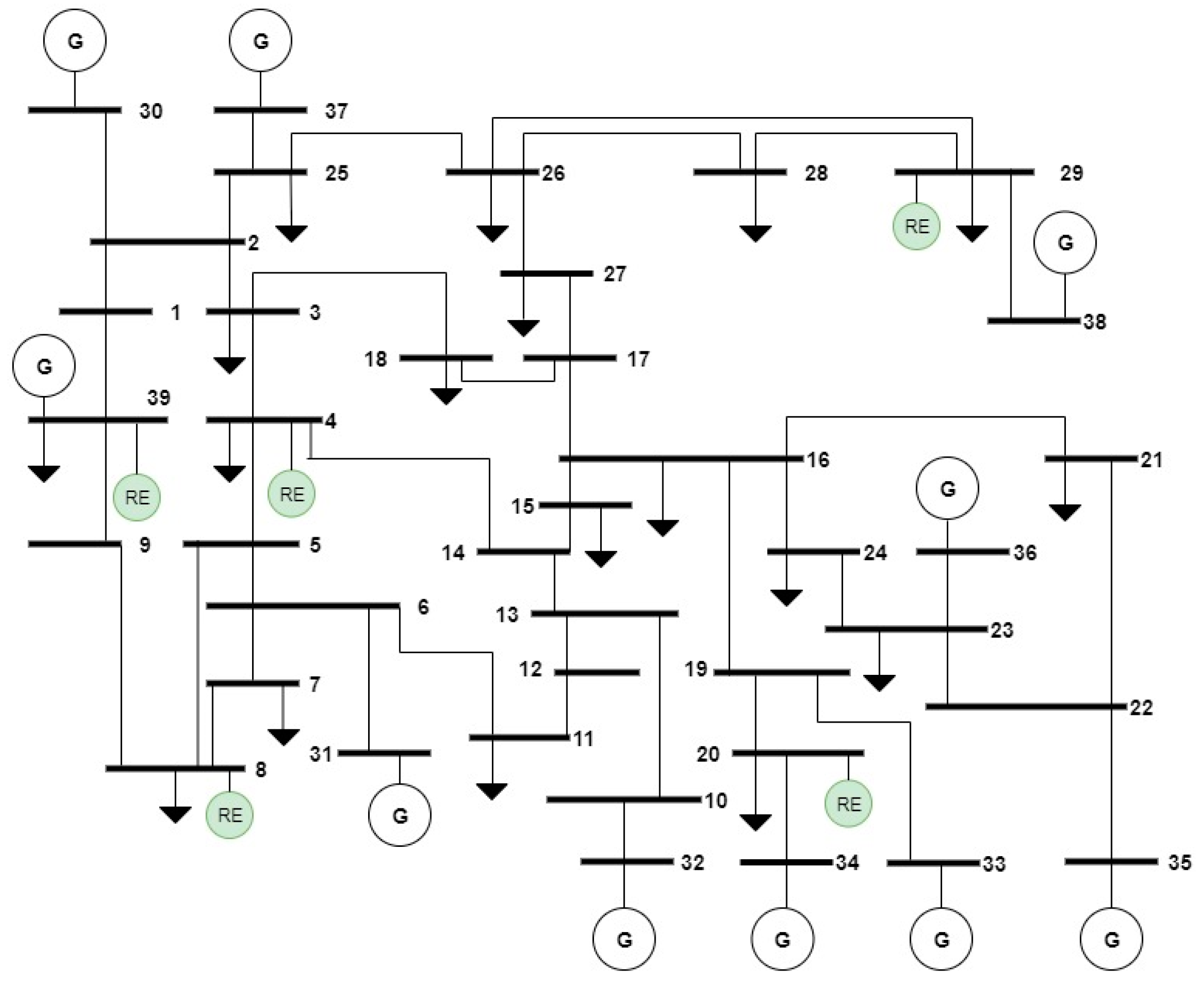
. The units of them are also given in Table 1. The test system used for this analysis was the modified New England 39 bus test-system including RE generation, the one-line diagram of which is shown in Figure 1. There are 39 buses and 10 synchronous generators in the New England test system. The five locations for the RE source that were considered in the simulations are also illustrated in Figure 1. The original case power flow without RE generation and dynamic data are provided in [22,23].

The state equations for each state variable are discussed in Section 2.1. The state equations are also called the differential equations of the system. The active and reactive power network equations for each bus are discussed in Section 2.2. The power network equations are also called the algebraic equations of the system. The formulation of the differential algebraic equations (DAEs) model of the system is shown in Section 2.3. From the DAE model, the system state matrix and the concept of eigenvalue sensitivity can be derived. This will serve as the foundation for the scenario screening framework that will be presented in Section 3.

2.1. State Variables

In this paper, each synchronous nonreference generator was represented by 10 state variables. The 10 state variables were rotor angle (${\delta }_i$), machine frequency (${\omega }_i$), quadrature axis emf ($E_{qi}^{\prime }$), direct axis emf ($E_{di}^{\prime }$), field winding voltage ($E_{fdi}$), AVR output ($V_{ri}$), exciter feedback ($R_{fi}$), prime mover mechanical power output ($P_{mi})$, and generator steam valve opening (${\mu }_i$). For reference generators, there will only be 9 state equations. There will be no state equation for the rotor angle of the reference generator since the rotor angles of the nonreference generators are referenced to the rotor angle of the reference generator.

The differential equations for the rotor angle (${\delta }_i$), machine frequency (${\omega }_i$), quadrature axis emf ($E_{qi}^{\prime }$), and direct axis emf ($E_{di}^{\prime }$) of the synchronous generators are written below [22]. The rotor angle of the mth generator is chosen as the reference angle of the system. In this paper, the generator in bus 39 was chosen as the reference generator.

$$\dot{{\delta }_i}=\left({\omega }_i-{\omega }_{sys}\right){\omega }_0,i = 1,\dots ,m-1;$$

(1)

$$\dot{{\omega }_i}=\frac{\left[P_{mi}-D_i\left({\omega }_i-{\omega }_{sys}\right)-\left(E_{qi}^{\prime }-X_{di}^{\prime }{I}_{di}\right)I_{qi}-\left(E_{di}^{\prime }+X_{qi}^{\prime }{I}_{qi}\right)I_{di}\right]}{M_i},i =1,\dots ,m;$$

(2)

$$\dot{E_{qi}^{\prime }}=\frac{\left[E_{fdi}-E_{qi}^{\prime }-\left(X_{di}-X_{di}^{\prime }\right)I_{di}\right]}{T_{d0i}},i =1,\dots ,m;$$

(3)

$$\dot{E_{di}^{\prime }} = \frac{\left[-E_{di}^{\prime }+\left(X_{qi}-X_{qi}^{\prime }\right)I_{qi}\right]}{T_{q0i}},i = 1,\dots ,m.$$

(4)

In the two-axis model shown in Equations (1)–(4), the stator transients were ignored. The machine direct axis ($I_{di}$) and quadrature axis currents ($I_{qi}$) are expressed [22] in the succeeding equations. $V$, $\theta$, and $\delta$ in the following equations refer to the bus voltage magnitude, bus voltage angle, and rotor angle respectively.

The nonreference generator ($i = 1,\dots ,m-1)$ is as follows:

$$I_{di} = \left[R_{si}{E}_{di}^{\prime }+E_{qi}^{\prime }{X}_{qi}^{\prime }-R_{si}{V}_i\sin \left({\delta }_i-{\theta }_i\right)-X_{qi}^{\prime }{V}_i\cos \left({\delta }_i-{\theta }_i\right)\right]/\left(R_{si}^2+X_{di}^{\prime }{X}_{qi}^{\prime }\right);$$

(5)

$$I_{qi} = \left[R_{si}{E}_{qi}^{\prime }-E_{di}^{\prime }{X}_{di}^{\prime }-R_{si}{V}_i\cos \left({\delta }_i-{\theta }_i\right)-X_{di}^{\prime }{V}_i\sin \left({\delta }_i-{\theta }_i\right)\right]/\left(R_{si}^2+X_{di}^{\prime }{X}_{qi}^{\prime }\right).$$

(6)

The reference generator ($i = m)$ is as follows:

$$I_{dm} = \left[R_{sm}{E}_{dm}^{\prime }+E_{qm}^{\prime }{X}_{qm}^{\prime }-R_{sm}{V}_m\sin \left(-{\theta }_m\right)-X_{qm}^{\prime }{V}_m\cos \left(-{\theta }_m\right)\right]/\left(R_{sm}^2+X_{dm}^{\prime }{X}_{qm}^{\prime }\right);$$

(7)

$$I_{qm} = \left[R_{sm}{E}_{qm}^{\prime }-E_{di}^{\prime }{X}_{dm}^{\prime }-R_{sm}{V}_m\cos \left(-{\theta }_m\right)-X_{dm}^{\prime }{V}_m\sin \left(-{\theta }_m\right)\right]/\left(R_{sm}^2+X_{dm}^{\prime }{X}_{qm}^{\prime }\right).$$

(8)

For the excitation control system of the synchronous generator, IEEE type DC-1 excitation system was used. The model for this excitation system [22] is shown in Equations (9)–(11). The following equations are for the field winding voltage ($E_{fdi}$), AVR output ($V_{ri}$), and exciter feedback ($R_{fi}$):

$$\dot{E_{fdi}} = \frac{\left[V_{ri}-\left[S_{ei}\left(E_{fdi}\right)\right]E_{fdi}\right]}{T_{ei}},i = 1,\dots ,m;$$

(9)

$$\dot{V_{ri}} = \frac{\left[-V_{ri}+K_{ai}\left(V_{refi}-V_i-R_{fi}\right)\right]}{T_{ai}},i = 1,\dots ,m;$$

(10)

$$\dot{R_{fi}} = \frac{\left[-R_{fi}-\left(K_{ei}+S_{ei}{E}_{fdi}\right)K_{fi}{E}_{fdi}{T}_{ei}^{-1}+K_{fi}{V}_{ri}{T}_{ei}^{-1}\right]}{T_{fi}},i = 1,\dots ,m.$$

(11)

The differential equation for the prime mover and speed governor model are shown in Equations (12) and (13) [22]. $P_{mi}$ refers to the prime mover mechanical power output, while ${\mu }_i$ is the mathematical expression for the physical representation of the generator steam valve opening. To compensate for any governor speed deviation from the reference speed (${\omega }_{ref})$, there is a corresponding change in ${\mu }_i$ depending on the speed difference and the droop constant ($R_i)$. The droop constant represents the speed governor inherent speed-droop characteristics [22]. A typical value for the droop constant is 5% droop.

$$\dot{P_{mi}} = T_{chi}^{-1}\left({\mu }_i-P_{mi}\right),i = 1,\dots ,m;$$

(12)

$$\dot{{\mu }_i} = T_{gi}^{-1}\left[P_{gsi}-\frac{{\omega }_i-{\omega }_{ref}}{R_i}-{\mu }_i\right],i= 1,\dots ,m.$$

(13)

2.2. Algebraic Variables

Consider a system with $n$buses, the network power equations for each bus of the system are shown as:

$$0=P_{gi}+P_{REi}-P_{li}-P_{ti},i = 1,\dots ,n;$$

(14)

$$0=Q_{gi}-Q_{li}-Q_{ti},i = 1,\dots ,n.$$

(15)

In this paper, the test system used was the New England test system and was composed of 39 buses. Since there is one algebraic equation each for the active power and reactive power, there will be 78 power network equations for this test system. By following this, a test system with n buses is expected to have 2n power network equations.

$P_{gi}$ and $Q_{gi}$ refer to the active power output and reactive power output of the generator at bus $i$. $P_{gi}$ and $Q_{gi}$ are zero if there is no generator in bus $i$. Otherwise, the equations for $P_{gi}$ and $Q_{gi}$ are shown below [22]. In (14), $P_{REi}$ stands for RE generation at bus $i$. In this paper, $P_{REi}$ was considered as a given parameter at a specific time period. Similar to the notation in the previous subsection, the variables $V$, $\theta$, and $\delta$ refer to the bus voltage magnitude, bus voltage angle, and rotor angle respectively.

The nonreference generator ($i = 1,\dots ,m-1)$ is as follows:

$$P_{gi} = I_{di}{V}_i\sin \left({\delta }_i-{\theta }_i\right)+I_{qi}{V}_i\cos \left({\delta }_i-{\theta }_i\right);$$

(16)

$$Q_{gi} = I_{di}{V}_i\cos \left({\delta }_i-{\theta }_i\right)-I_{qi}{V}_i\sin \left({\delta }_i-{\theta }_i\right).$$

(17)

The reference generator ($i = m)$ is as follows:

$$P_{gm} = I_{dm}{V}_m\sin \left(-{\theta }_m\right)+I_{qm}{V}_m\cos \left(-{\theta }_m\right);$$

(18)

$$Q_{gm} = I_{dm}{V}_m\cos \left(-{\theta }_m\right)-I_{qm}{V}_m\sin \left(-{\theta }_m\right).$$

(19)

$P_{ti}$ and $Q_{ti}$ refer to the total network active power and reactive power injections at the ith bus respectively. These equations are similar to the equations used in the power flow analysis [24]. $Y_{ij}$ and ${\gamma }_{ij}$ in the following equations refer to the bus admittance magnitude and angle respectively.

$$P_{ti} = {\sum }_{j = 1}^n\left|V_i\right|\left|V_j\right|\left|Y_{ij}\right|\cos \left({\theta }_i-{\theta }_j-{\gamma }_{ij}\right),i=1,\dots ,n;$$

(20)

$$Q_{ti} = {\sum }_{j = 1}^n\left|V_i\right|\left|V_j\right|\left|Y_{ij}\right|\sin \left({\theta }_i-{\theta }_j-{\gamma }_{ij}\right),i=1,\dots ,n.$$

(21)

The active power load model and the reactive power load model are given as shown in Equations (22) and (23) respectively [22]. $P_{lo,i}$, $Q_{lo,i}$, and $V_{o,i}$ refer to the initial load active power, initial load reactive power, and initial load voltage respectively. $KP, KQ$, and $K_{freq}$ are load factors.

$$P_{li} = P_{lo,i}\left[K{P}_{1i}+K{P}_{2i}\left(\frac{V_i}{V_{o,i}}\right)+K{P}_{3i}{\left(\frac{V_i}{V_{o,i}}\right)}^2\right]\left(1+K_{freq,i}\left({\omega }_m-1\right)\right),i= 1,\dots ,n;$$

(22)

$$Q_{li} = Q_{lo,i}\left[K{Q}_{1i}+K{Q}_{2i}\left(\frac{V_i}{V_{o,i}}\right)+K{Q}_{3i}{\left(\frac{V_i}{V_{o,i}}\right)}^2\right]\left(1+K_{freq,i}\left({\omega }_m-1\right)\right),i= 1,\dots ,n.$$

(23)

By inspecting the active power and reactive power network equations, it can be seen that the equations are in terms of $V$ and $\theta$. Because of this, $V$ and $\theta$ are called the algebraic variables of the system.

2.3. System State Matrix and Eigenvalue Sensitivity

The general form of the differential and algebraic equations (DAEs) describing the power system is shown as [22]:

$$\dot{\Delta x} = f\left(x,y,a\right),$$

(24)

$$0 = g\left(x,y,a\right),$$

(25)

where$f$ and $g$ refer to the set of differential and algebraic equations respectively. $f$ and $g$ can be represented in terms of the state variables ($x$), algebraic variables ($y$), and the control parameter ($a$). From Section 2.1 and Section 2.2, $x$ and $\mathrm{y}$ are defined as the set of differential and algebraic variables. In this paper, the control parameter is the RE variation in the system.

$$x = \left\{\delta , \omega , E_q^{\prime }, E_d^{\prime }, E_{fd}, V_r, R_f, P_m, \mu \right\};$$

(26)

$$y = \left\{V, \theta \right\}.$$

(27)

The solution of the DAE model is the equilibrium point of the system. By linearizing the DAE model around the equilibrium point, the resulting equations are shown in state matrix form in Equation (28). The matrix elements $f_x$, $f_y$, $g_x$, and $g_y$ are called the Jacobian matrices of the system. The symbol $\Delta$ represents parameter deviation.

$$\left[\begin{array}{c}\dot{\Delta x}\\ 0\end{array}\right] = \left[\begin{array}{cc}{f}_x& f_y\\ g_x& g_y\end{array}\right]\left[\begin{array}{c}\Delta x\\ \Delta y\end{array}\right].$$

(28)

By assuming that the Jacobian matrix $g_y$ is nonsingular, the variable $\Delta y$ can be eliminated in the system of equations. The new equation for $\Delta y$ is substituted in the equation for $\dot{\Delta x}$. The resulting equation is shown in Equation (30). From Equation (30), the equation for the system state matrix $A_s$ is derived.

$$\Delta y = -g_y^{-1}{g}_x\Delta x;$$

(29)

$$\dot{\Delta x} = \left[f_x-f_y{g}_y^{-1}{g}_x\right]\Delta x;$$

(30)

$$A_s = \left[f_x-f_y{g}_y^{-1}{g}_x\right].$$

(31)

The sensitivity of the eigenvalue $\mathsf{\lambda }$ with respect to system parameter $\alpha$ is given by Equation (32) [8]. Eigenvalue sensitivity depicts how the system eigenvalues are affected by a change in a system parameter.

$$\frac{\partial \mathsf{\lambda }}{\partial \alpha } = {\psi }^T\frac{\partial A_s}{\partial \mathsf{\alpha }}\varphi .$$

(32)

In Equation (32), it is shown that the eigenvalues and eigenvectors of the system state matrix $A_s$ are used to determine the eigenvalue sensitivity of the system. $\psi$ pertains to the left eigenvector, while $\varphi$ pertains to the right eigenvector of the system state matrix $A_s$.

3. Renewable Energy (RE) Generation Scenario Screening Framework Based on Eigenvalue Sensitivity

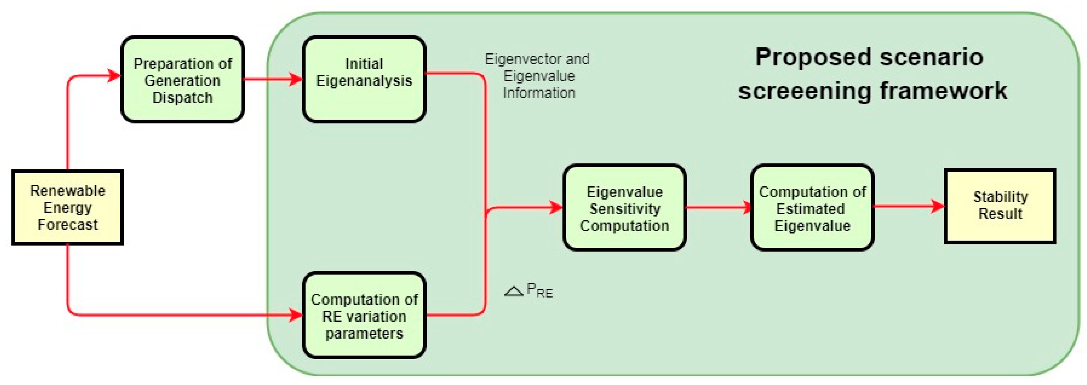
The overview of the proposed scenario screening framework is shown in Figure 2. The generation dispatch was scheduled based on the day-ahead forecast of RE. The initial eigenanalysis was then analyzed according to the scheduled dispatch. Based on the initial eigenanalysis, the eigenvalues with the lowest damping ratios and eigenvalues with the largest real parts were considered as critical eigenvalues. The critical eigenvalues were monitored closely because they were the most probable candidates to cross the imaginary axis first. The eigenvalue sensitivity with respect to the renewable energy was simulated based on the eigenvalue and eigenvector information from the initial eigenanalysis. This is discussed further in Section 3.1.

RE generation scenarios were defined by the RE location, average forecasting error, forecasting error standard deviation and average forecasted RE output. The computation for the $\Delta P_{RE}$ input was based on the RE generation scenario variables. The formulations for the $\Delta P_{RE}$ and RE generation scenario variables are shown in Section 3.2.

The estimated eigenvalues were calculated by adding the eigenvalue sensitivity information to the initial critical eigenvalues. If an estimated eigenvalue was found in the right complex plane, then the system might be unstable in this RE generation scenario, so it requires more detailed simulation and countermeasure determination. Likewise, if all eigenvalues were found in the left complex plane, then the system is said to be stable in this RE generation scenario.

The formulation for calculating the uncertainty of the real part of critical eigenvalues is discussed in Section 3.3. Additional discussion and a detailed flowchart are presented in Section 3.4.

3.1. Eigenvalue Sensitivity with Respect to Variation of RE

The sensitivity of the eigenvalues with respect to RE was calculated because it could determine the effect of the variable RE to the eigenvalues of the power system. The eigenanalysis of the base case scenario was evaluated first to determine the initial eigenvalues and eigenvectors of the system. The eigenvalues and the eigenvectors were used to determine the sensitivity of eigenvalues. From Equation (32), the sensitivity of the critical eigenvalue ${\lambda }_c$ with respect to RE generation $P_{RE}$ can be derived. The resulting equation is shown in Equation (33).

$$\frac{\partial {\lambda }_c}{\partial P_{RE}} = {\psi }^T\frac{\partial A_s}{\partial P_{RE}}\varphi .$$

(33)

To determine the partial derivative of the system state matrix $A_s$ with respect to $P_{RE}$, the derivative of the system state matrix with respect to $V$ and $\delta$ were used in this method. $V$ refers to the voltage magnitude and $\delta$ refers to the phase angle.

$$\frac{\partial A_s}{\partial P_{RE}} = \frac{\partial A_s}{\partial \left|V\right|}\frac{\partial \left|V\right|}{\partial P_{RE}}+\frac{\partial A_s}{\partial \delta }\frac{\partial \delta }{\partial P_{RE}}.$$

(34)

When connected to the grid, the added RE acts to decrease the active power being supplied by the generators to the loads. $P_{RE}$ is added in the Jacobian matrix used for power flow analysis. $\frac{\partial \left|V\right|}{\partial P_{RE}}$ and $\frac{\partial \delta }{\partial P_{RE}}$ can be derived from the inverse of the Jacobian matrix.

$$\left[\begin{array}{c}\Delta P\\ \Delta Q\end{array}\right] = \left[\begin{array}{cc}{J}_1& J_2\\ J_3& J_4\end{array}\right]\left[\begin{array}{c}\Delta \delta \\ \Delta \left|V\right|\end{array}\right];$$

(35)

$$\left[\begin{array}{c}\Delta \delta \\ \Delta \left|V\right|\end{array}\right] = {\mathit{J}}^{-1}\left[\begin{array}{c}\Delta P\\ \Delta Q\end{array}\right].$$

(36)

By taking the derivative of the system state matrix with respect to $V$, Equation (31) is changed to the following equation:

$$\frac{\partial A_s}{\partial \left|V\right|} = \left[\frac{\partial f_x}{\partial \left|V\right|}-\frac{\partial f_y}{\partial \left|V\right|}{g}_y^{-1}{g}_x-f_y\frac{\partial g_y^{-1}}{\partial \left|V\right|}{g}_x-f_y{g}_y^{-1}\frac{\partial g_x}{\partial \left|V\right|}\right].$$

(37)

In [25], a simplified expression for $\frac{\partial g_y^{-1}}{\partial \left|V\right|}$ was proposed. By substituting the expression $\frac{\partial g_y^{-1}}{\partial \left|V\right|}=-g_y^{-1}\frac{\partial g_y}{\partial \left|V\right|}{g}_y^{-1}$ in Equation (37), the new expression for $\frac{\partial A_s}{\partial \left|V\right|}$ is shown in Equation (38).

$$\frac{\partial A_s}{\partial \left|V\right|} = \frac{\partial f_x}{\partial \left|V\right|}-\frac{\partial f_y}{\partial \left|V\right|}{g}_y^{-1}{g}_x+f_y{g}_y^{-1}\frac{\partial g_y}{\partial \left|V\right|}{g}_y^{-1}{g}_x-f_y{g}_y^{-1}\frac{\partial g_x}{\partial \left|V\right|}.$$

(38)

Likewise, an analysis is done to get the derivative of the system state matrix $A_s$ with respect to $\delta$.

$$\frac{\partial A_s}{\partial \mathsf{\delta }} = \frac{\partial f_x}{\partial \mathsf{\delta }}-\frac{\partial f_y}{\partial \mathsf{\delta }}{g}_y^{-1}{g}_x+f_y{g}_y^{-1}\frac{\partial g_y}{\partial \mathsf{\delta }}{g}_y^{-1}{g}_x-f_y{g}_y^{-1}\frac{\partial g_x}{\partial \mathsf{\delta }}.$$

(39)

3.2. RE Generation Scenario

A RE generation scenario is a set of conditions that describes how much the actual RE output deviates from the forecasted RE output. In some cases, the actual output differs from the forecasted output because of the intermittency of RE. Obviously, several RE generation scenarios need to be checked in operation. The framework of this paper can quickly evaluate the impact of each scenario, in terms of small-signal stability, to screen critical RE generation scenarios.

Each RE generation scenario is defined by RE location, average forecasting error (mean absolute percent error, MAPE), forecasting error standard deviation (${\sigma }_{err}$), and average forecasted RE output ($\overline{P_{RE}^{for}}$). The location of the RE source is included as part of the scenario because it also affects the generator loading and the exchange of power within the grid.

$P{E}_{k,t}$ refers to the percent error between the forecasted ($P_{RE}^{for}$) and actual ($P_{RE}^{act}$) RE output for time slot $t$ in the kth RE generation scenario.

$$P{E}_{k,t} = \left|\frac{P_{RE,k}^{act,t}-P_{RE,k}^{for,t}}{P_{RE,k}^{act,t}}\right|100 [\%].$$

(40)

The formulations for solving the MAPE, ${\sigma }_{err}$, and $\overline{P_{RE}^{for}}$ for each RE generation scenario are shown in the following equations.

$$MAP{E}_k=\frac{{\sum }_{t = 1}^{n}P{E}_{k,t}}{n} 100 [\%];$$

(41)

$${\sigma }_{err,k}=\sqrt{\frac{{\sum }_{t = 1}^n{\left(P{E}_{k,t}-MAP{E}_k\right)}^2}{n}}[\%];$$

(42)

$$\overline{P_{RE}^{for}}=\frac{{\sum }_{t = 1}^n{P}_{RE,k}^{for,t}}{n}.$$

(43)

The corresponding $\mathsf{\Delta }{P}_{RE}$ for each RE generation scenario can be evaluated using Equation (44). When setting $\mathrm{K}$ to 3, 99.7% of all probable forecasting error margins will be covered in the analysis.

$$\mathsf{\Delta }{P}_{RE,k}=\pm \overline{P_{RE}^{for}}\left(MAP{E}_k+\mathrm{K}{\sigma }_{err,k}\right).$$

(44)

The estimated critical eigenvalues can be calculated using Equation (45). The calculated eigenvalue sensitivity $\frac{\partial {\lambda }_c}{\partial P_{RE}}$from Equation (33) is multiplied by the change in the RE generation, $\mathsf{\Delta }{P}_{RE}$. This term is added to the initial critical eigenvalue ${\lambda }_c$ to estimate the movement of the eigenvalue.

$${\lambda }_{c,e}={\lambda }_c+\frac{\partial {\lambda }_c}{\partial P_{RE}} \mathsf{\Delta }{P}_{RE}.$$

(45)

Using Equation (45), all critical eigenvalues are estimated with respect to $\mathsf{\Delta }{P}_{RE}$. Then, the framework checks whether there are any estimated eigenvalues in the right side of the complex plane. If there are eigenvalues in the right side of the complex plane, then the system might be unstable in this RE generation scenario, and it requires more detailed analysis in terms of small-signal stability.

3.3. Uncertainty of the Real Part of Critical Eigenvalues

In [26], a framework for quantifying the uncertainty of the transmission reliability margin was proposed with respect to uncertain parameters. In this paper, a similar formulation was employed to evaluate the uncertainty of the real part of the critical eigenvalues with respect to the RE generation scenarios. The formulation for the uncertainty $U_c$ of the real term of a critical eigenvalue,${\lambda }_c$, is shown in Equation (46). In the evaluation, the sensitivity of the real part with respect to renewable energy and the variance of the renewable energy are both used.

$$U_c=\sqrt{{\sum }_{k = 1}^l{\left(\frac{\partial Real({\lambda }_c)}{\partial P_{RE,k}}\right)}^2{\left(\mathsf{\Delta }{P}_{RE,k}\right)}^2},$$

(46)

where $l$ is the total number of considered RE generation scenarios.

3.4. Additional Discussion on the Proposed Framework

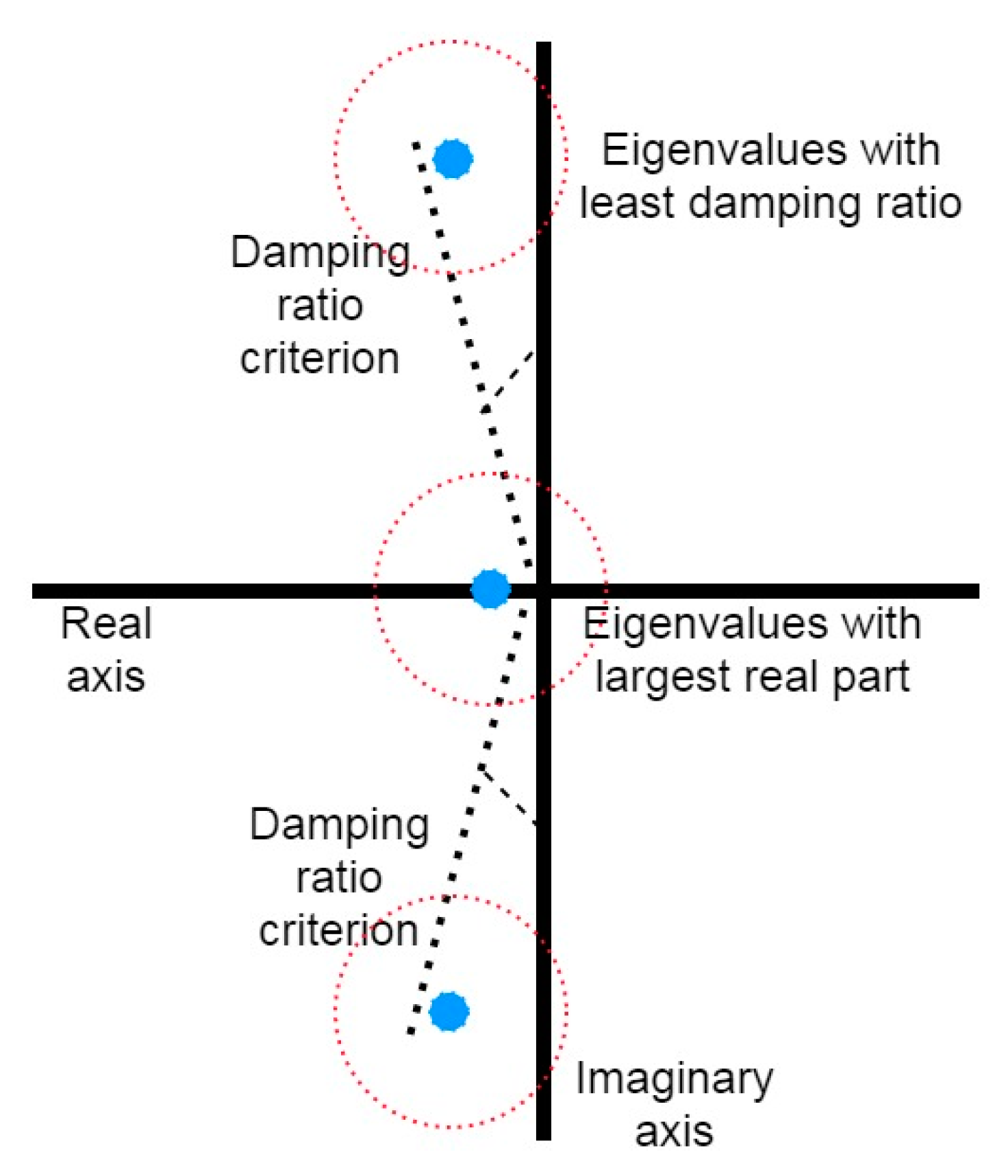
As shown in Equation (45), the sensitivity of the eigenvalues is used to calculate the estimated eigenvalues. Figure 3 depicts how eigenvalue sensitivity can be used to screen RE generation scenarios. The blue circle in Figure 3 represents the critical eigenvalues of the system. The critical eigenvalues can either be eigenvalues with the lowest damping ratios or eigenvalues with the largest real parts. The black dashed lines represent the damping ratio margin that will serve as the criteria to determine which eigenvalues are considered as critical. Depending on the variability of RE in the system for a given scenario, the system eigenvalues may cross the imaginary axis and move to the right half of the complex plane. The area within the red circle represents the possible location of the eigenvalues as a result of the added variable RE. If the eigenvalues are found to be at the right side of the complex plane or if they cross the imaginary axis, the system is unstable for that scenario.

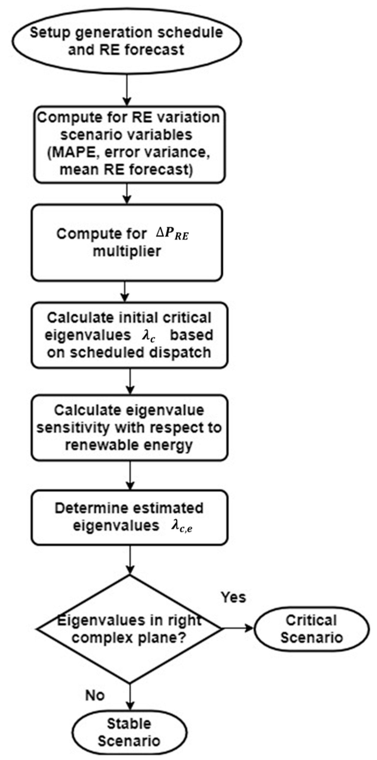
A flowchart is presented in Figure 4 to summarize the process of screening RE generation scenarios.

4. Simulation Results and Analysis

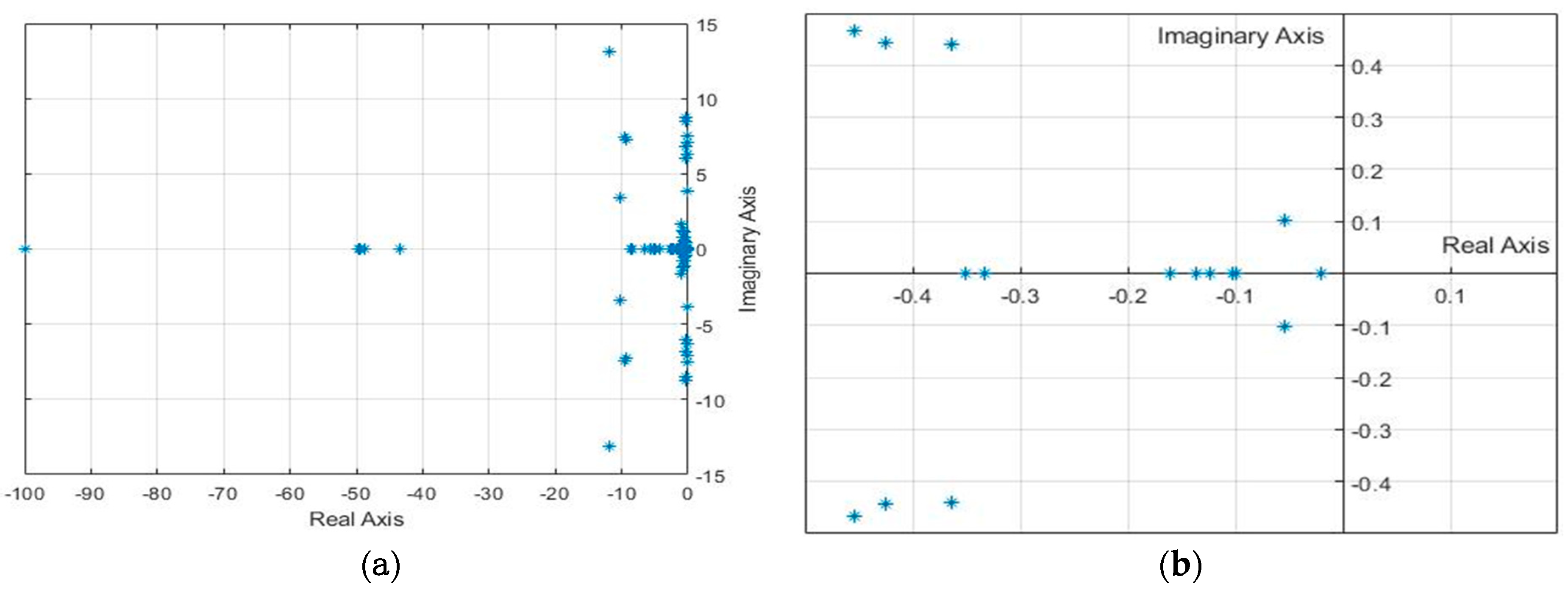
As in Figure 1, the modified New England system was adopted in the simulation. The eigenvalues of the New England Test System without any RE penetration are shown in Figure 5 below. The eigenvalue analysis shows that the system had 89 eigenvalues: 41 of which were real eigenvalues and the other 48 were complex eigenvalues (24 complex eigenvalue pairs). Eighty-nine eigenvalues were expected because each nonreference generator was represented by 9 state equations, and the reference generator was represented by 8 state equations.

In Figure 5a, all eigenvalues are shown. The eigenvalues were all in the left-hand side of the imaginary axis. Hence, in this case, the system was stable. The system will be unstable if any of the system eigenvalues cross the imaginary axis and move to the right-hand side of the complex plane. Some of the closest eigenvalues near the origin are shown in Figure 5b. These eigenvalues were considered as critical eigenvalues and may have the highest probability of crossing the imaginary axis first, depending on the amount of RE added to the system.

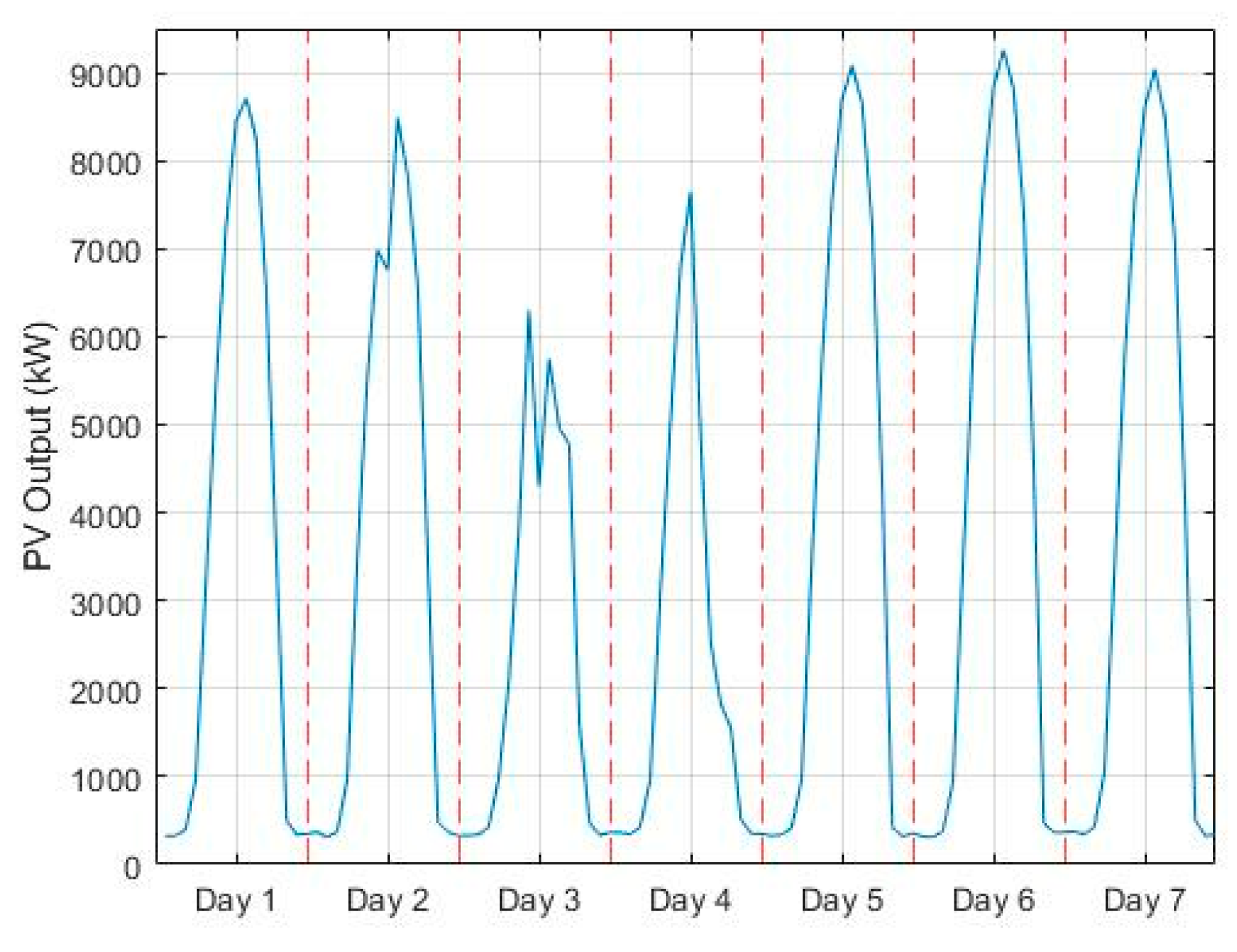
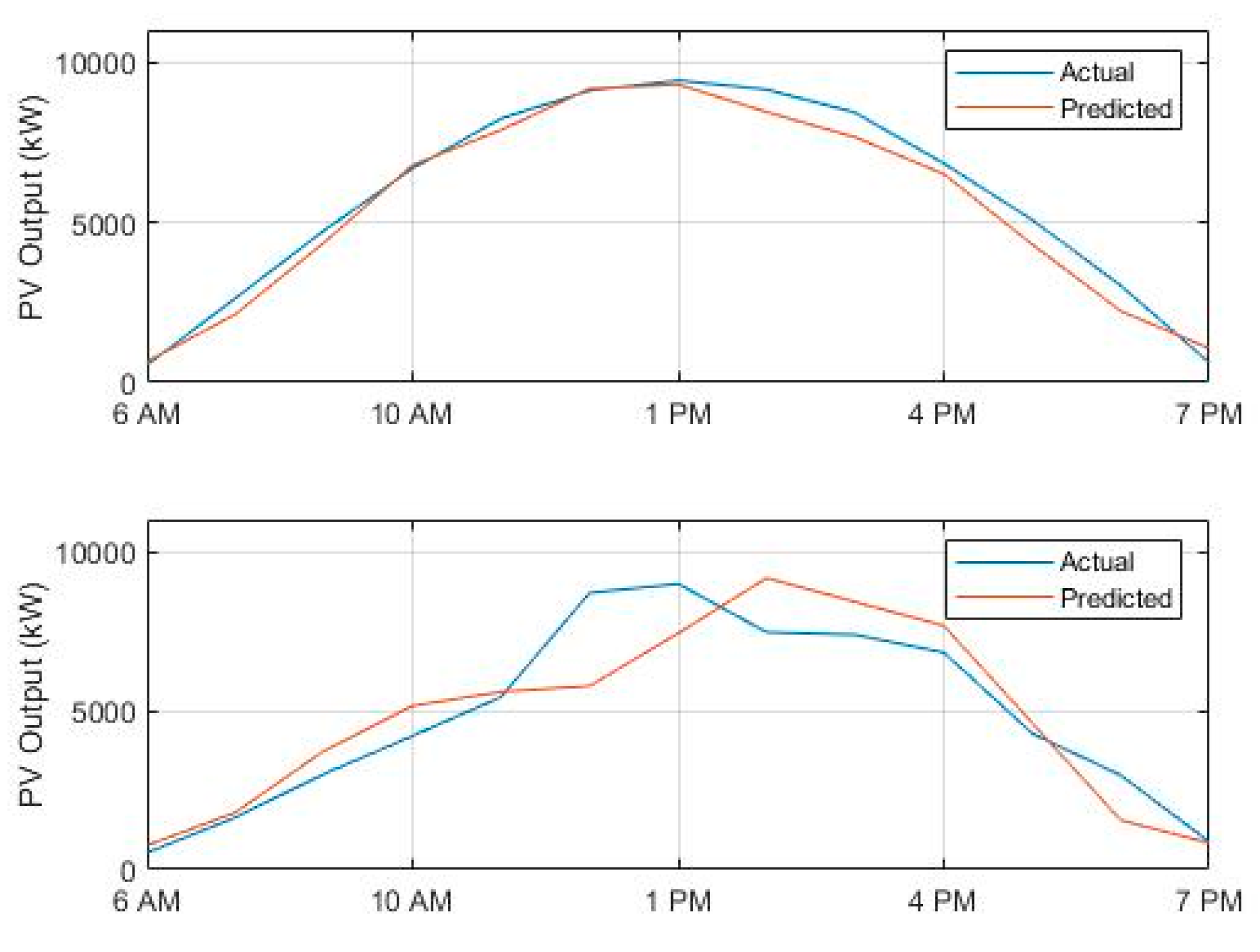
The type of RE considered in the simulation for this paper was solar energy. The long short-term memory (LSTM) model was used in this paper to predict the photovoltaic (PV) cell system output based on historical one-year PV output data and cloud cover data. The standard deviation of the error between the actual and predicted PV output (${\sigma }_{err})$, average forecasted PV output ($\overline{P_{RE}^{for}}),$and average forecasting error (MAPE) were used to define the scenario conditions for the proposed method. A sample one-week snapshot of the training data is shown in Figure 6. The total PV output per day is also shown in Figure 6. While in Figure 7, a sample prediction and actual curve of the total PV plant for a sunny and cloudy day are shown. The amount of cloud cover affects PV generation output, and this makes it harder for system operators to forecast PV accurately [27].

The first three (3) simulated scenario cases are shown below:

Scenario 1: PV plant in bus 20, MAPE = 15%, ${\sigma }_{err}$ = 8%, $\overline{P_{RE}^{for}}$ = 5.41 pu;

Scenario 2: PV plant in bus 8, MAPE = 15%, ${\sigma }_{err}$ = 8%, $\overline{P_{RE}^{for}}$ = 5.41 pu;

Scenario 3: PV plant in bus 4, MAPE = 13%, ${\sigma }_{err}$ = 22%, $\overline{P_{RE}^{for}}$ = 5.65 pu.

In the first two scenarios, the PV resource was placed first on bus 20 and then changed to bus 8 to compare results. The same RE generation conditions were assumed for the first two scenarios. In the third scenario, the PV resource was moved to bus 4 with higher variability of PV assumed in the system. The results of the proposed method were verified by comparing it with the eigenanalysis results.

In this paper, the least damping ratio criterion, used to classify which eigenvalues are considered critical, was 0.10 or 10%. The damping ratio of each eigenvalue ($\mathsf{\lambda }=\mathsf{\sigma }+\mathrm{j}\mathsf{\omega })$is given by Equation (47) [8]. For the largest real parts criterion, eigenvalues with real part greater than −0.10 were considered as critical eigenvalues.

$$\zeta = \frac{-\sigma }{\sqrt{{\sigma }^2+{\omega }^2}}.$$

(47)

The results of the simulations for the three scenarios are summarized in Table 1,

Table 2. Critical eigenvalues and their estimated values considering RE variation (Scenario 1).

Critical Eigenvalues
Initial Eigenvalues	Damping Ratio	Estimated Eigenvalues	Eigenanalysis Verification
−0.020396	−	−0.020602	−0.020401
−0.0545 ± j0.1006	46.33%	−0.0527 ± j0.1009	−0.0544 ± j0.1005
−0.098483	−	−0.098324	−0.098482
−0.099908	−	−0.099909	−0.099906
−0.099950	−	−0.099940	−0.099949
−0.1030 ± j7.0492	1.46%	−0.1011 ± j7.0495	−0.1049 ± j7.0513
−0.1475 ± j3.8144	3.86%	−0.1521 ± j3.8156	−0.1372 ± j3.7936
−0.2138 ± j6.3527	3.36%	−0.2118 ± j6.3527	−0.2098 ± j6.3710
−0.2188 ± j7.4223	2.95%	−0.2183 ± j7.4224	−0.2219 ± j7.4099
−0.2749 ± j5.9925	4.58%	−0.2765 ± j5.9928	−0.2778 ± j5.9816
−0.2952 ± j6.8491	4.31%	−0.2932 ± j6.8478	−0.3036 ± j6.8400
−0.3501 ± j8.4344	4.15%	−0.3460 ± j8.4326	−0.3492 ± j8.3686
−0.4199 ± j8.6828	4.83%	−0.4203 ± j8.6813	−0.4282 ± j8.6256
−0.4264 ± j8.7167	4.89%	−0.4280 ± j8.7170	−0.4537 ± j8.6902

and

Table 3. Critical eigenvalues their estimated values considering RE variation (Scenario 2).

Critical Eigenvalues
Initial Critical Eigenvalues	Damping Ratio	Estimated Eigenvalues	Eigenanalysis Verification
−0.020388	−	−0.020535	−0.020385
−0.0545 ± j0.1006	47.63%	−0.0559 ± j0.1003	−0.0544 ± j0.1005
−0.098481	−	−0.098361	−0.098479
−0.099909	−	−0.099911	−0.099906
−0.099949	−	−0.099944	−0.099948
−0.1038 ± j7.0460	1.47%	−0.1022 ± j7.0463	−0.1052 ± j7.0462
−0.1915 ± j4.0371	4.74%	−0.1979 ± j4.0381	−0.1977 ± j4.0936
−0.2086 ± j6.3657	3.27%	−0.2100 ± j6.3652	−0.2017 ± j6.3809
−0.2209 ± j7.4225	2.97%	−0.2210 ± j7.4228	−0.2245 ± j7.4098
−0.2871 ± j6.0769	4.72%	−0.2895 ± j6.0770	−0.2978 ± j6.1165
−0.3071 ± j6.8680	4.47%	−0.3089 ± j6.8691	−0.3231 ± j6.8702
−0.3554 ± j8.4827	4.19%	−0.3539 ± j8.4821	−0.3600 ± j8.4555
−0.4179 ± j8.7060	4.79%	−0.4185 ± j8.7052	−0.4218 ± j8.6594
−0.4205 ± j8.7197	4.82%	−0.4217 ± j8.7192	−0.4475 ± j8.6963

. The results shown in the initial critical eigenvalues column are based on the scheduled dispatch. If an eigenvalue had a damping ratio of less than 0.10 or 10%, or if the real part of the eigenvalue was greater than −0.1, the eigenvalue was considered as a critical eigenvalue. The corresponding damping ratio for each complex eigenvalue is shown in the next column. Critical eigenvalues were given special importance in the analysis because they were the most probable candidates to cross the imaginary axis first. If any of these eigenvalues crossed the imaginary axis to the right-hand side of the complex plane, then the system might be unstable in this scenario. The estimated eigenvalues column shows the result of the proposed method by adding the eigenvalue sensitivity with respect to PV variability to the initial critical eigenvalues. These results were then verified with the results of the eigenanalysis with the corresponding PV generation.

In the results shown in Table 2, the assumed condition was that the scheduled dispatch included a mean PV output of 5.41 pu in bus 20. The values shown in the estimated eigenvalues column were evaluated using the proposed method and without solving for the eigenanalysis solution. Based on the results, the proposed method showed that the eigenvalues were still in the left-hand side of the complex plane. As such, the system was considered stable in this scenario. To verify this result, PV output was then added to the system, and an eigenanalysis was done to determine the eigenvalues of the system in this case. The results are shown in the eigenanalysis verification column. The eigenanalysis result also showed that the eigenvalues were in the left-hand side of the complex plane. Hence, Scenario 1 was considered as a stable scenario as both estimated eigenvalues and the eigenanalysis verification showed the same result.

To test if the method will be applicable in other locations in the system, the same analysis was done with the same scenario conditions but with a different PV location. In the simulation results shown in Table 3, the same scenario conditions were used, but the PV location was changed to bus 8. It showed that the results of the proposed method agreed with the results of the eigenanalysis verification for this scenario as well. The system was shown to be stable for the assumed conditions in this scenario.

In the last scenario, the PV bus was changed to bus 4, but with a higher scheduled PV output mean and higher PV output variability. The scheduled dispatch included a mean PV output of 5.65 pu. The results for the analysis done with this scenario are shown in

Table 4. Critical eigenvalues and their estimated values considering RE variation (Scenario 3).

Critical Eigenvalues
Initial Critical Eigenvalues	Damping Ratio	Estimated Eigenvalues	Eigenanalysis Verification
−0.020391	−	−0.020513	−0.020388
−0.0545 ± j0.1006	47.65%	−0.0538 ± j0.1005	−0.0543 ± j0.1004
−0.1017 ± j7.0482	1.44%	−0.0959 ± j7.0478	−0.1035 ± j7.0507
−0.098482	−	−0.098252	−0.098477
−0.099909	−	−0.100026	−0.099903
−0.099950	−	−0.100067	−0.099948
−0.1842 ± j3.9922	4.61%	−0.1933 ± j3.9948	−0.1950 ± j4.0954
−0.2131 ± j6.3702	3.34%	−0.2266 ± j6.3624	−0.2008 ± j6.4134
−0.2200 ± j7.4230	2.96%	−0.2358 ± j7.4309	−0.2289 ± j7.3893
−0.3551 ± j8.4897	4.18%	−0.2934 ± j8.4717	−0.3655 ± j8.4227
−0.3041 ± j6.8745	4.42%	−0.3123 ± j6.8848	−0.3411 ± j6.8798
−0.2858 ± j6.0708	4.70%	−0.3129 ± j6.0656	−0.3138 ± j6.1570
−0.4146 ± j8.7258	4.75%	−0.4128 ± j8.7892	−0.4779 ± j8.6659
−0.4177 ± j8.7133	4.79%	−0.4227 ± j8.6258	−0.4301 ± j8.5995

. For increased variability of the PV output, the proposed method showed that the system was stable in this scenario since all eigenvalues were in the left-hand side of the complex plane. The results agreed with the eigenanalysis verification in this scenario.

In the evaluation of the uncertainty of the real part of the critical eigenvalues, two (2) additional scenarios were considered, as shown below:

Scenario 4: PV plant in bus 29, MAPE = 13%, ${\sigma }_{err}$ = 22%, $\overline{P_{RE}^{for} }$= 5.65 pu;

Scenario 5: PV plant in bus 39, MAPE = 13%, ${\sigma }_{err}$ = 22%, $\overline{P_{RE}^{for}}$ = 8.48 pu.

By considering the five scenarios, the uncertainty of the real part of the critical eigenvalues can be evaluated using Equation (44). The real part of the five largest and smallest real parts of the critical eigenvalues for each scenario are tabulated in

Table 5. Uncertainty of the real part of the estimated critical eigenvalues with respect to PV variation.

Real Part of Critical Eigenvalues, Estimated					${\mathit{U}}_{\mathit{c}}$
Scenario 1 Bus 20	Scenario 2 Bus 8	Scenario 3 Bus 4	Scenario 4 Bus 29	Scenario 5 Bus 39
−0.4280	−0.4217	−0.4128	−0.4153	−0.3927	0.0341
−0.4203	−0.4185	−0.4227	−0.4098	−0.2955	0.0594
−0.3460	−0.3539	−0.2934	−0.3796	−0.2830	0.0858
−0.2932	−0.3089	−0.3123	−0.3001	−0.2111	0.0282
−0.2765	−0.2895	−0.2266	−0.2690	−0.3565	0.0616
−0.0999	−0.0999	−0.1000	−0.1000	−0.1001	0.0002
−0.0983	−0.0984	−0.0983	−0.0981	−0.0984	0.0005
−0.0527	−0.0559	−0.0538	−0.0568	−0.0541	0.0036
−0.0206	−0.0205	−0.0205	−0.0208	−0.0207	0.0006
−0.1521	−0.1979	−0.1933	−0.1595	0.0111	0.0182

.

The uncertainty for the real part of each critical eigenvalue are shown in the last column of the table. In Scenario 4, the RE generation scenario was similar to Scenario 3, but the PV location was moved from bus 4 to bus 29. After evaluating the sensitivity of the critical eigenvalues with respect to PV generation, the proposed scenario screening framework determined that Scenario 4 was a stable scenario as all of the estimated critical eigenvalues were in the left complex plane.

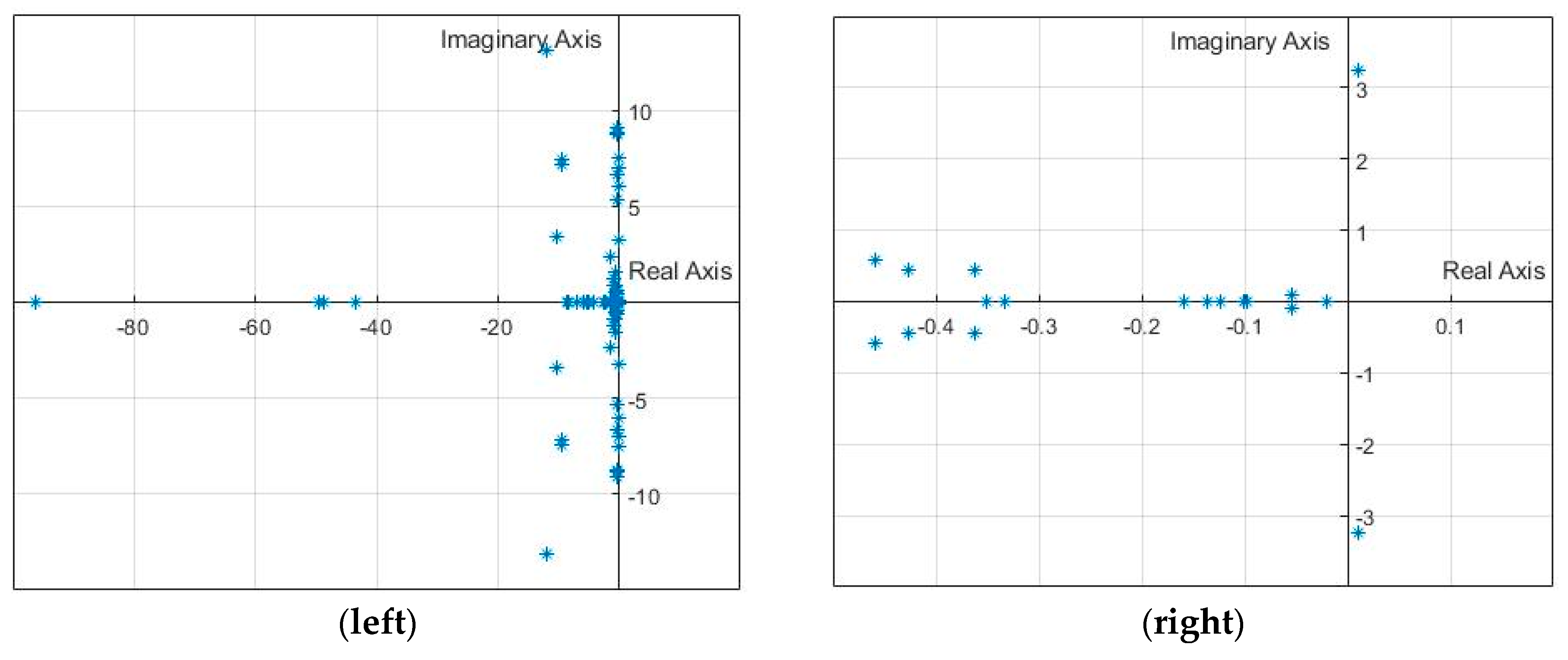
While in Scenario 5, the scheduled PV generation was higher compared to the other scenarios, and the PV location was moved to bus 39. After applying the proposed method, it was determined that there was an estimated critical eigenvalue in the right complex plane. If an eigenvalue is found in the right complex plane, the system might be unstable in this scenario. The results of both scenarios agreed with the eigenanalysis verification. The system eigenvalues of the critical scenario are shown in the left image of Figure 8. The eigenvalues near the imaginary axis are shown in the right image of Figure 8 for easier visualization. It can be seen from this image that a complex eigenvalue pair crossed the imaginary axis, therefore making the scenario unstable and critical.

The significance of the uncertainty results showed that, by considering the variation in the PV output in any of the considered PV locations and the sensitivity of the eigenvalues, the real part of the critical eigenvalues varied by the uncertainty value. This is a measure of how the critical eigenvalues were affected on a system-level perspective.

The results of the proposed scenario screening framework and their run times are tabulated in

Table 6. Summary of RE scenario screening framework results.

Scenario	Stability Result	Run Time (s)
Scenario 1	Stable	0.202571
Scenario 2	Stable	0.199852
Scenario 3	Stable	0.203656
Scenario 4	Stable	0.198558
Scenario 5	Unstable	0.204091

. The simulations were done on a computer with a 3.30 GHz Intel processor and 8 GB RAM.

All scenarios, except Scenario 5, were stable scenarios since the estimated critical eigenvalues in these scenarios were found in the left complex plane. Since there was a critical eigenvalue that crossed the imaginary axis in Scenario 5, the system might be unstable in this scenario, according to small-signal stability rules, and it requires further detailed simulations. The run times of the proposed method were similar to those of the analytical methods using the original New England test system in [16]. However, it should be noted that the proposed framework had a different applicability, which was to quickly screen critical RE generation scenarios in terms of small-signal stability, and not only to calculate eigenvalue sensitivity.

For critical scenarios determined by the proposed framework, countermeasure determination was needed with several control parameters such as active power injection with energy storage systems (ESSs) and generation re-dispatch. As in [28,29], the ESS capability of local energy supplying systems including microgrids could increase the operational efficiency by reducing uncertainty of RE. In addition, it could improve system stability, which might be threatened by RE intermittence, if the local systems with ESS followed the signals to meet the required control amount as ancillary service providers. As in [30,31], the concept of microgrids also included the role of energy hub and energy router. If power injections from those energy hubs are properly scheduled to minimize the negative impacts by RE intermittence in several security issues, system security can be enhanced as well. The proposed method of this paper can be used to quickly filter alarming situations in term of small-signal stability; hence, adequate control signals of required power injection are determined.

5. Conclusions

This paper presents the framework for screening RE generation scenarios in terms of small-signal stability. Instead of performing eigenanalyses for all possible operating points, the proposed screening framework adopted eigenvalue sensitivity with respect to renewable generation and checked if the system might violate the small-signal stability rules by RE fluctuation. The case studies using the proposed method showed that it could quickly determine whether there might be the possibility of instability for several RE scenario conditions such as different bus locations and different RE variability levels. For all the scenarios in the simulation, the proposed method showed that the results agreed with the eigenanalysis verification with the corresponding operating points. The proposed method was very helpful to find critical scenarios that may possibly lead to severe conditions. By using the information from the method, a more detailed analysis may be done in terms of small-signal stability, especially for unstable scenarios. Thus, the method can be used in system planning and operational planning stages to evaluate the effect of different RE generation scenarios and to quickly filter critical ones. As a result, system engineers could come up with adequate countermeasures against those cases to improve the grid reliability and to mitigate the security risks.