A Data-Driven Scheduling Approach for Hydrogen Penetrated Energy System Using LSTM Network

Abstract

Intra-day control and scheduling of energy systems require high-speed computation and strong robustness. Conventional mathematical driven approaches usually require high computation resources and have difficulty handling system uncertainties. This paper proposes two data-driven scheduling approaches for hydrogen penetrated energy system (HPES) operational scheduling. The two data-driven approaches learn the historical optimization results calculated out using the mixed integer linear programing (MILP) and conditional value at risk (CVaR), respectively. The intra-day rolling optimization mechanism is introduced to evaluate the proposed data-driven scheduling approaches, MILP data-driven approach and CVaR data-driven approach, along with the forecasted renewable generation and load demands. Results show that the two data-driven approaches have lower intra-day operational costs compared with the MILP based method by 1.17% and 0.93%. In addition, the combined cooling and heating plant (CCHP) has a lower frequency of changing the operational states and power output when using the MILP data-driven approach compared with the mathematical driven approaches.

1. Introduction

The continuing development of the energy system has made the conventional electric power system move forward to a multi-carrier energy system including electric, gas, heating, and cooling [1]. Along with the increasing penetration of renewable energy, uncertainties and fluctuations of the energy system are becoming serious challenges to network operators [2]. It is important to explore efficient ways of balancing renewable generations and consumer energy demands. Benefiting from the storage stability, energy density, and transformation capability (Power-to-Gas) of hydrogen, the hydrogen penetrated energy system (HPES) is attracting great attention in recent years [3,4,5]. The hydrogen can be used as the fuel not only for the fuel-cell battery but also for the combined cooling and heating plant (CCHP) when mixed with natural gas, the so-called Hydrogen Compressed Nature Gas (HCNG) [6,7]. However, due to the tight coupling characteristics of the HPES and the little research on HCNG powered CCHP, it is difficult to establish mathematical models of the equipment within HPES in high accuracy, and the operational scheduling and adjustment for HPES also require high computation resources. Thus, Artificial-Intelligence assisted scheduling and control approaches are considered as a potential way of managing the HPES.

A number of studies have been performed for multi-carrier energy systems using mathematical based optimization approach [8,9,10,11]. In article [8] the authors model the multi-carrier energy system as a non-linear model and perform the coordinated scheduling for the energy resources using the heuristic optimization methodology. The approach in [12] proposed an optimal scheduling approach for integrated energy system with consideration of energy storage systems and ancillary services. The regionally integrated energy system is modeled as a linear mathematical model which can be solved by software packages and commercial optimization systems, YALMIP, and CPLEX. In article [13], the authors proposed a conditional value at risk (CVaR) based multi-objective optimization approach for hydrothermal system considering the uncertainties of energy demands. Results show that the CVaR based approach is applicable for hydrothermal integrated energy systems, and the risk level of the system operation can be decreased. The approach in [14] proposed a bi-level economic dispatch method for nature gas-electricity coupled energy systems to minimize its operational cost. The lower level model is transferred by Karush-Kuhn-Tucher (KKT) conditions and added to the upper-level model, which make the whole model as a mixed integer linear programing (MILP) formulation and can be solved by most of the commercial optimization software packages. Other mathematical-driven approaches for optimizing the integrated energy system operation have been presented in [15,16,17,18].

The aforementioned mathematical-driven scheduling and control approaches for a multi-carrier energy system require high-computational resources, especially when the system has a large number of non-linear components or is on a large-scale. Therefore, when online scheduling and control of the HPES is needed, the mathematical-driven approaches sometimes are not able to meet the speed requirements. Thus, some data-driven based approaches are proposed that learn the scheduling experience offline and control the system online [19,20,21,22]. In article [19], the authors proposed a reinforcement learning control approach for building heating systems. The results show that the proposed method is able to handle the control of building systems with various ambient temperatures in a very short time. A similar reinforcement learning approach for community energy management is proposed in [23], of which the fuzzy control concept is introduced into the Q-learning algorithm to handle the rewards of learning process. The approach in [20] proposed a random forest-based model predictive control approach for building energy optimization and climate control. The case studies show that the energy can be saved up to 49.2% within the building. A number of data-driven approaches have been used in the building energy management system as mentioned above and achieve reasonable performance. The HPES is a more complex system than building or community energy systems, and the scheduling and management of HPES have similar characteristics to building energy systems, but few data-driven control approaches are investigated to optimize the operation of multi-carrier energy system or integrated energy system. Thus, it is worth exploring the potential of data-driven control approaches in the HPES.

In this paper, the detailed models of HPES are established at first. After then two data-driven operational scheduling approaches based on Long Short-Term Memory (LSTM) are introduced. The two approaches learn and formulate the operational scheduling models based on the MILP and CVaR optimization results of the HPES respectively. To validate the performance of the two approaches, the two approaches are evaluated in the intra-day operation of a typical HPES which requires high computation speed and has more uncertainties. The contributions of this paper can be summarized as below.

(1)

This paper proposed two LSTM based operational scheduling and control approaches for HPES.

(2)

This paper evaluated the performance of the proposed approaches in the intra-day operation of the HPES.

(3)

The intra-day operational cost, intra-day equipment operational scheduling and the computational speed of the proposed scheduling and control approaches are analyzed in detail.

The remainder of this paper is organized as follows: Section 2 describes the modeling of HPES in MILP and CVaR, the data-driven approaches operational flow for HPES, and the established process of data-driven scheduling approach based on LSTM. Section 3 performs the detailed analysis of proposed approaches compared with conventional mathematical driven approaches. Section 4 concludes the advantages and shortcomings of the proposed data-driven approaches.

2. Materials and Methods

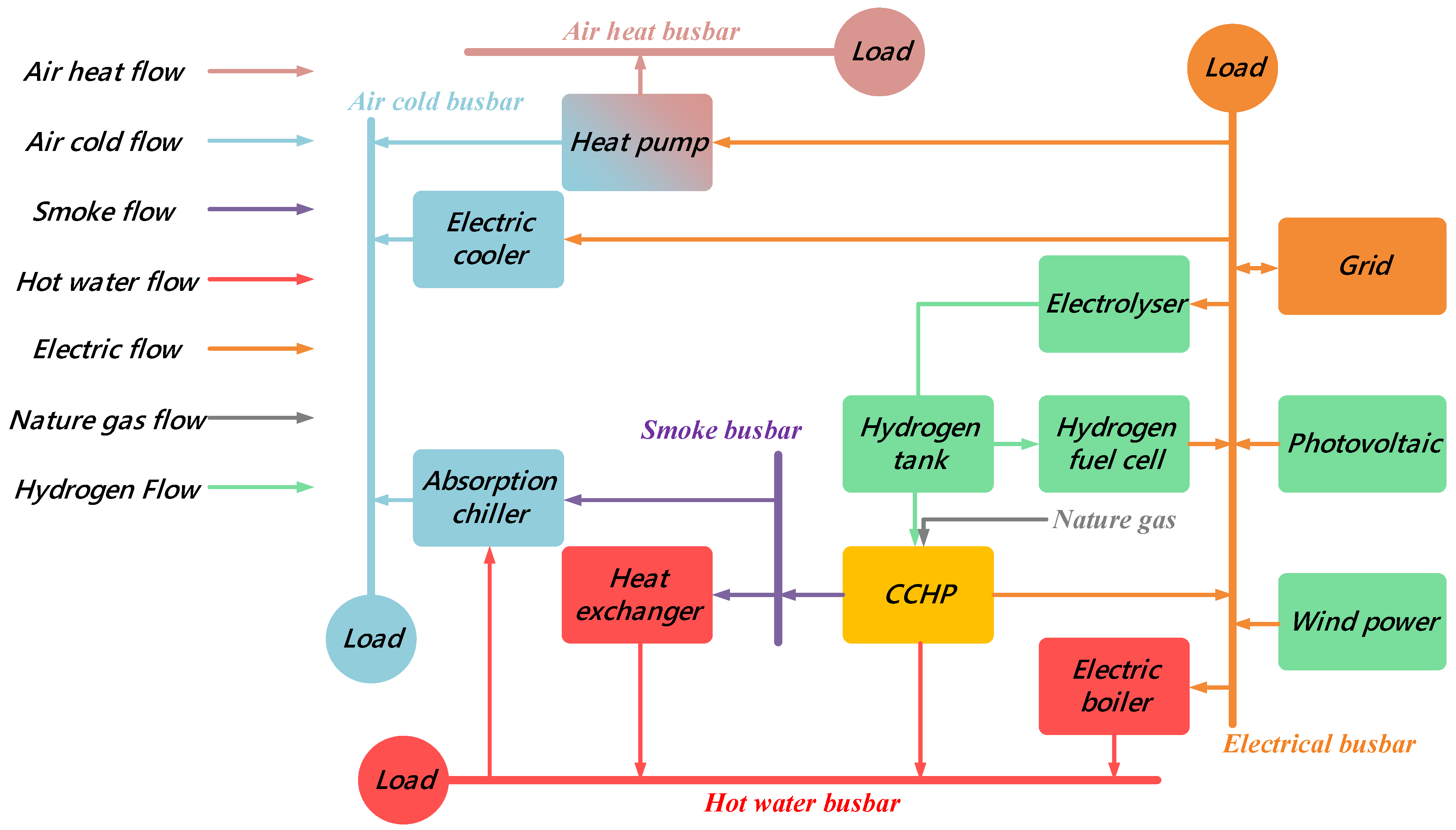
2.1. Hydrogen Penetrated Energy System (HPES)

HPES is an integrated energy system that can convert the surplus electricity into hydrogen which can be stored and re-used at the right time. Such energy systems can facilitate the consumption of the wind and photovoltaic (PV) energy and reduce the grid pressure and system operating cost. Figure 1. shows the structure of the HPES where the hydrogen is generated via water electrolyzing within an electrolyzer and subsequently stored in the hydrogen tank(s). The hydrogen can be mixed with natural gas as the input fuel for combined cooling and heating power (CCHP) units or used independently for hydrogen fuel cells. The CCHP units can supply electrical energy, hot water, and smoke whilst other devices such as electric boiler and heat exchanger can only provide hot water. The electric cooler and absorption chiller are used for cooling. The heat pump can be used for both cooling and heating.

2.2. HPES Mathematical Modelling

The LSTM model needs to learn the historical optimization scheme in order to produce a control strategy. Hence, it is inevitable to model the HPES and collect the optimization scheme from the historical data. The LSTM learns the data that is optimized by either the MILP or CVaR method and the effects are analyzed separately.

The HPES generally contains five energy-carrier busbars including the electrical busbar, hot water busbar, smoke busbar, hot air busbar, cold air busbar. The energy balance of each busbar is expressed by Equations (1)–(5):

$$L_E+P_{grid.s}+P_{HP}+P_{EC}+P_{EL}+P_{EB}=P_{PV}+P_W+P_{grid.b}+P_{HFC}+P_{CHP},$$

(1)

$$L_{TW}+Q_{AC.water}=Q_{HFC}+Q_{HE.water}+Q_{CHP.water}+Q_{EB},$$

(2)

$$Q_{AC.smoke}+Q_{HE.smoke}=Q_{CHP.smoke}$$

(3)

$$L_{ca}=Q_{HP.c}+Q_{EC}+Q_{AC}$$

(4)

$$L_{ta}=Q_{HP.h}$$

(5)

The hydrogen generated from the electrolyzer can be used by the CCHP unit and the fuel cell. More specifically, the CCHP unit takes the gas mixture consisting of natural gas and hydrogen as the input fuel. The device constraints are presented in Equations (6)–(14). Note that Equations (9)–(11) are derived from experimental data and show the relationship between the electrical power of CCHP and the flow rate of natural gas ($v_{ng}$) and hydrogen ($v_{H_2.CHP}$).

$$v_{gb}=v_{ng}+v_{H_2.CHP}$$

(6)

$$0\le v_{ng}\le v_{ng}^{max}$$

(7)

$$0\le v_{H_2.CHP}\le {\epsilon }^{max}·v_{gb}$$

(8)

$$P_{CHP}=3.031v_{ng}+1.019v_{H_2.CHP}$$

(9)

$$Q_{CHP.water}=6.086v_{ng}-0.5331v_{H_2.CHP}$$

(10)

$$Q_{CHP.smoke}=0.9914v_{ng}+0.3012v_{H_2.CHP}$$

(11)

$$P_{CHP}^{min}·{\mu }_{CHP}\le P_{CHP}\le P_{CHP}^{max}·{\mu }_{CHP}$$

(12)

$$-R·\Delta t\le P_{CHP}^1-P_{CHP}^0\le R·\Delta t$$

(13)

$${\mu }_{CHP}\in \left\{0,1\right\}$$

(14)

The constraints of the hydrogen tank are indicated by Equations (15)–(17). The change in the amount of hydrogen in the hydrogen storage tank is related to the speed and time of the charge and discharge gas, as shown in Equation (15). The hydrogen storage tank also has maximum capacity constraints and charge and discharge gas maximum speed constraints as shown in Equations (16) and (17). In the model described herein, the hydrogen storage tank charging rate is the same as the electrolyzer producing hydrogen gas velocity and is therefore not listed in the hydrogen storage tank constraint.

$$V_{H_2}^1=V_{H_2}^0+v_{ht.i}·\Delta t-v_{ht.o}·\Delta t$$

(15)

$$0\le V_{H_2}\le V_{H_2}^{max}$$

(16)

$$0\le v_{ht.o}\le v_{ht.o}^{max}$$

(17)

It is necessary for the electrolyzer and fuel cell to satisfy the relationship between its power and the flow rate of hydrogen as stated in Equation (18), as well as the upper and lower limits of the hydrogen flow rate as depicted in Equation (19).

$$P=v·\delta$$

(18)

$$v^{min}\le v\le v^{max}$$

(19)

Other devices should primarily meet the relationship between power and efficiency or energy efficiency ratio (EER) as shown in Equation (20). The electro-thermal efficiency of devices should also satisfy the upper and lower limits as shown in Equations (21) and (22). The power exchanged between the grid and the HPES also needs to meet the upper and lower limit of Equations (21) and (22).

$$Q=P·\eta$$

(20)

$$P^{min}\le P\le P^{max}$$

(21)

$$Q^{min}\le Q\le Q^{max}$$

(22)

Equations (23)–(25) state how the system operating costs can be calculated and the MILP objective function of the day-ahead economic scheduling can be determined. The price of each part is the unit price multiplied by the time. The optimization goal is to minimize the operating cost of the system under the conditions of busbar constraints and equipment constraints.

$$C_{ng}=c_{ng}·{\displaystyle \sum }_{t=1}^{24}\left(v_{ng}^t·\Delta t\right)$$

(23)

$$C_{grid.b}={\displaystyle \sum }_{t=1}^{24}\left(P_{grid.b}^t·\Delta t·c_{grid.b}^t\right)$$

(24)

$$C_{grid.s}=c_{grid.s}·{\displaystyle \sum }_{t=1}^{24}\left(P_{grid.s}^t·\Delta t\right)$$

(25)

$$\mathrm{Objective}:\min \left(C_{ng}+C_{grid.b}-C_{grid.s}\right)$$

$$\mathrm{Constraints}:\left(1\right)–\left(25\right)$$

When the CVaR approach is used, the value of CVaR shall be calculated using Equations (26)–(28). This paper defines the objective function of CVaR as the CVaR whose operating cost exceeds the expected operating cost. In the traditional CVaR method, the value of the value at risk (VaR) is first required, which makes the solving process more complicated. According to [24], CVaR can be calculated under the condition that the VaR value is unknown. This method is applied to the solution process. Two intermediate variables $\xi$ and ${\varphi }^i$ are used to calculate CVaR, where $\xi$ is used instead of VaR. The proposed objective function is equivalent to the conventional method, as shown in Equations (26)–(28). The corresponding objective function is the sum of the expected running cost and the CVaR. Note that $\beta$ is the weight of CVaR.

$$\mathrm{Objective}:\min \xi +\frac{1}{N·\left(1-\alpha \right)}·{\displaystyle \sum }_{i=1}^N{\varphi }^i$$

(26)

$$\mathrm{Constraints}:{\varphi }^i\ge C_{Bill}^i-E_{Bill}-\xi$$

(27)

$${\varphi }^i\ge 0$$

(28)

$$\mathrm{Objective}:E_{Bill}+\beta ·R_{CVaR}$$

$$\mathrm{Constraints}:\left(1\right)–\left(25\right),\left(27\right),\left(28\right)$$

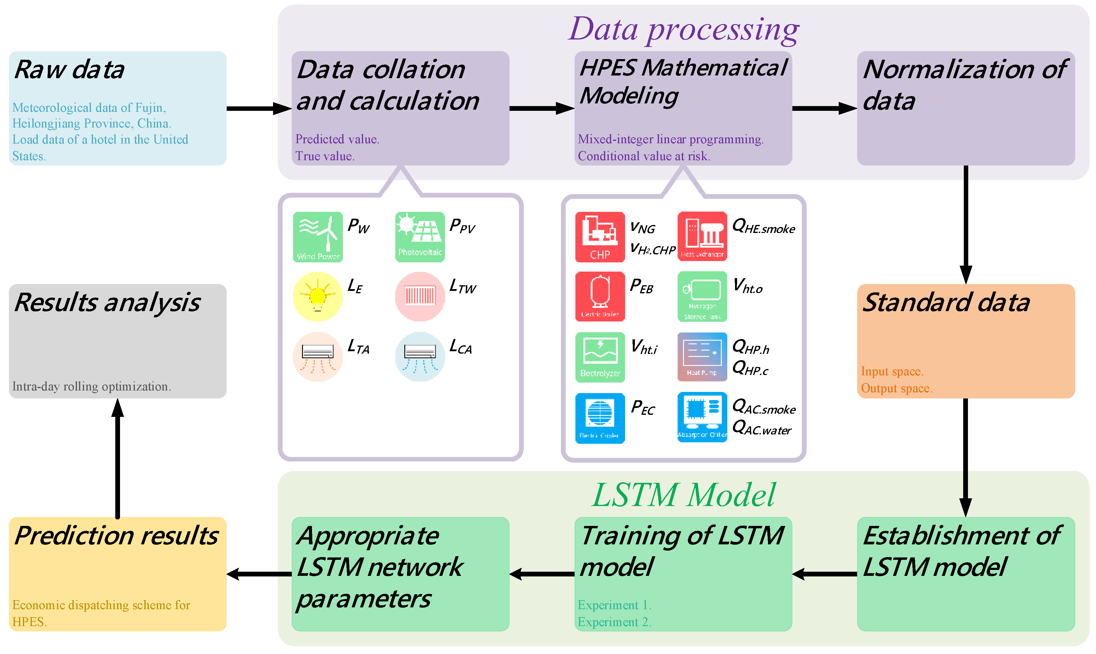
2.3. Data-Driven Approach for HPES Scheduling

Long Short-Term Memory (LSTM) is suitable for processing and predicting the time series related problems and the running optimization problems of an HPES are time-correlated. Based on the historical data, this paper proposes to use LSTM to solve the day-ahead economic scheduling problems of a HEPS.

The procedure of the data-driven approach for HPES scheduling is shown in Figure 2. The characteristics of the LSTM model (i.e., the predicted value of the PV power, wind power, and load) are obtained through the integration and calculation of the raw data, which forms the input space of the model. After the optimization computation, the label of the LSTM model (i.e., the day-ahead economic scheduling scheme of the integrated energy system) can be derived, which establishes the output space of the model. The input and output space are normalized so that they can be used as the standard data for the LSTM model. Appropriate LSTM network parameters are obtained by training the LSTM model. Consequently, the day-ahead economic scheduling scheme of the HPES can be achieved from the predicted values of the PV power, wind power, and load. In order to verify the performance of the optimized scheduling scheme generated by the LSTM, this paper establishes the intra-day rolling optimization model of the HPES and compares the intra-day rolling results of three different day-ahead economic scheduling schemes based on LSTM, mixed integer linear programming (MILP) and conditional value at risk (CVaR), respectively.

2.4. LSTM Based Approach

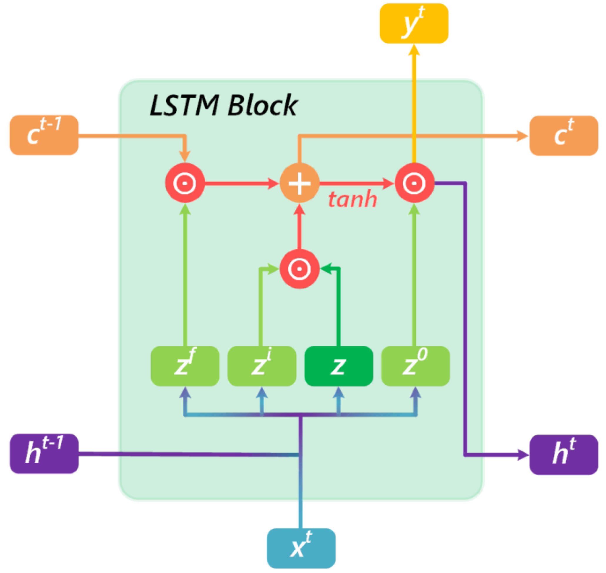
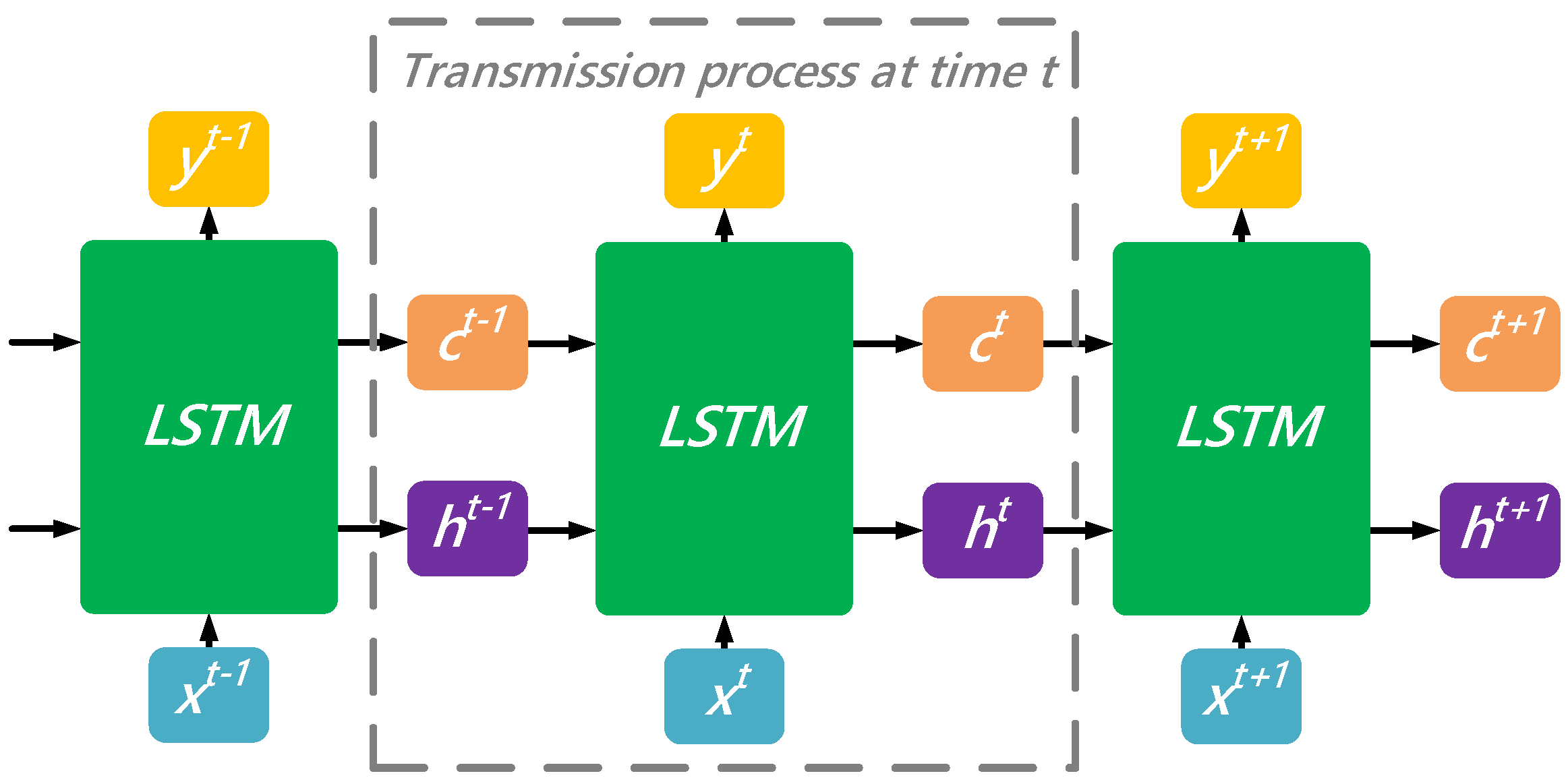
2.4.1. Introduction of LSTM

The LSTM artificial neural network is a recurrent neural network (RNN) proposed by Hochreiter and promoted by Alex Graves [25]. The long short-term memory function is added so that the information will not be attenuated, which solves the gradient vanishing and exploding problems during the long sequence training process of RNN. Figure 3 illustrates the network structure of the LSTM. There are two states in LSTM: the long term memory $c^t$ and the short term memory $h^t$. An LSTM unit has three inputs and three outputs. For time t, the inputs are the data input $x^t$ at time t and the long term memory $c^{t-1}$ and short term memory $h^{t-1}$ at a previous time (t − 1) whilst the outputs are the data output $y^t$, long term memory $c^t$ and short term memory $h^t$ at time t.

The internal architecture of an LSTM unit is indicated in Figure 4 where four training states are achieved via combining the current input $x^t$ and the $h^{t-1}$ that is outputted from the previous time t − 1. $z^f$, $z^i$ and $z^0$ represents the results of the forget gate, input gate and output gate which are derived by applying the sigmoid function to the product of the weight (e.g., $W^f$, $W^i$ or $W^0$) and the concatenated vector [$x^t$, $h^{t-1}$]. The results are between 0 and 1. z is the network input which is converted to a value between −1 and 1 by applying the tanh function to the product of the weight $W$ and the concatenated vector [$x^t$, $h^{t-1}$].

$$z^f=sigmoid\left(W^f\left[h^{t-1},x^t\right]\right)$$

(29)

$$z^i=sigmoid\left(W^i\left[h^{t-1},x^t\right]\right)$$

(30)

$$z^0=sigmoid\left(W^0\left[h^{t-1},x^t\right]\right)$$

(31)

$$z=tanh\left(W\left[h^{t-1},x^t\right]\right)$$

(32)

There are three steps within the LSTM:

The “forget” step selectively drops the input from the previous node and use $z^f$ as the forget gate controller to decide how much information of $c^{t-1}$ will be forgotten. Note that the value of $z^f$ is between 0 and 1. Value 0 indicates “completely forget this” whilst 1 indicates “completely keep this”.

The “input” step selectively takes the current input $x^t$ where the content of the current input is denoted by z and $z^i$ is used as the input gate controller. Note that the value of $z^i$ is between 0 and 1. Value 0 indicates “completed drop this” whilst 1 indicates “completed take this”.

The “output” step is mainly controlled by $z^0$ and the output $y^t$ is achieved by transforming $h^t$.

$$c^t=c^{t-1}⨀z^f+z^i⨀z$$

(33)

$$h^t=z^0⨀tanh\left(c^t\right)$$

(34)

$$y^t=sigmoid\left(W^{\prime }{h}^t\right)$$

(35)

2.4.2. LSTM based Control Strategy

According to the model established in Section 3.1, the MILP and CVaR based day-ahead economic scheduling scheme for the HPES can be obtained from the historical data of load, PV power and wind power (including actual and predicted values). The input space of the LSTM network consists of six variables that are related to the load, PV power, and wind power. These six variables include the electrical load $L_E$, hot water load $L_{TW}$, cold air load $L_{ca}$, hot air load $L_{ta}$, PV power $P_{PV}$ and wind power $P_W$. In order to reduce the number of labels, eleven variables that can represent the operation of all devices are selected and all other variables of the system can be derived accordingly. The eleven representative system variables are the natural gas consumption rate $v_{ng}$, hydrogen consumption rate of the CCHP unit $v_{H_2.CHP}$, electrical power of the electric boiler $P_{EB}$, smoke power consumed by the heat exchanger $Q_{HE.smoke}$, smoke power consumed by the absorption chiller $Q_{AC.smoke}$, hot water power consumed by the absorption chiller $Q_{AC.water}$, hydrogen generation rate of the electrolyzer $v_{hst.i}$, hydrogen output rate of the hydrogen storage tank $v_{hst.o}$, heating power generated by the heat pump $Q_{HP.h}$, cooling power generated by the heat pump $Q_{HP.c}$ and electrical power of the electric refrigerator $P_{EC}$. Using the input and output space to train the LSTM network, appropriate network parameters can be obtained and the day-ahead economic scheduling scheme of the HPES can thus be deduced from the future predicted data.

This paper denotes the learning process of the MILP based optimization method as experiment 1 whilst the learning process of the CVaR based optimization method as expression 2.

Experiment 1: the input space contains the predicted values of the load, PV power, and wind power whilst the output space is the operating strategy that is achieved by applying the MILP optimization to the actual values of the load, PV power, and wind power.

Experiment 2: the input space contains the predicted values of the load, PV power, and wind power whilst the output space is the operating strategy that is achieved by applying the CVaR optimization to the predicted values of the load, PV power, and wind power.

3. Results and Discussion

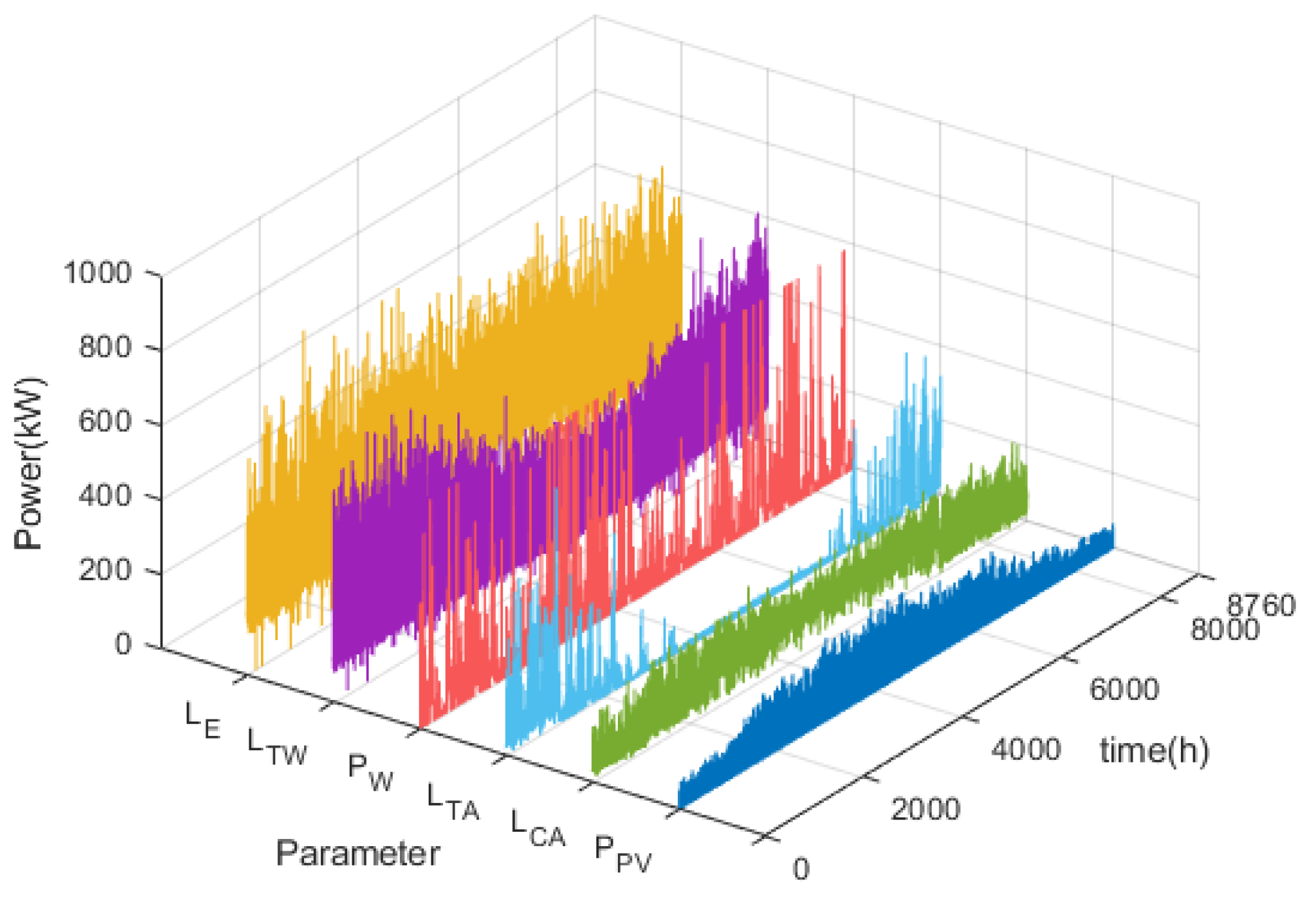
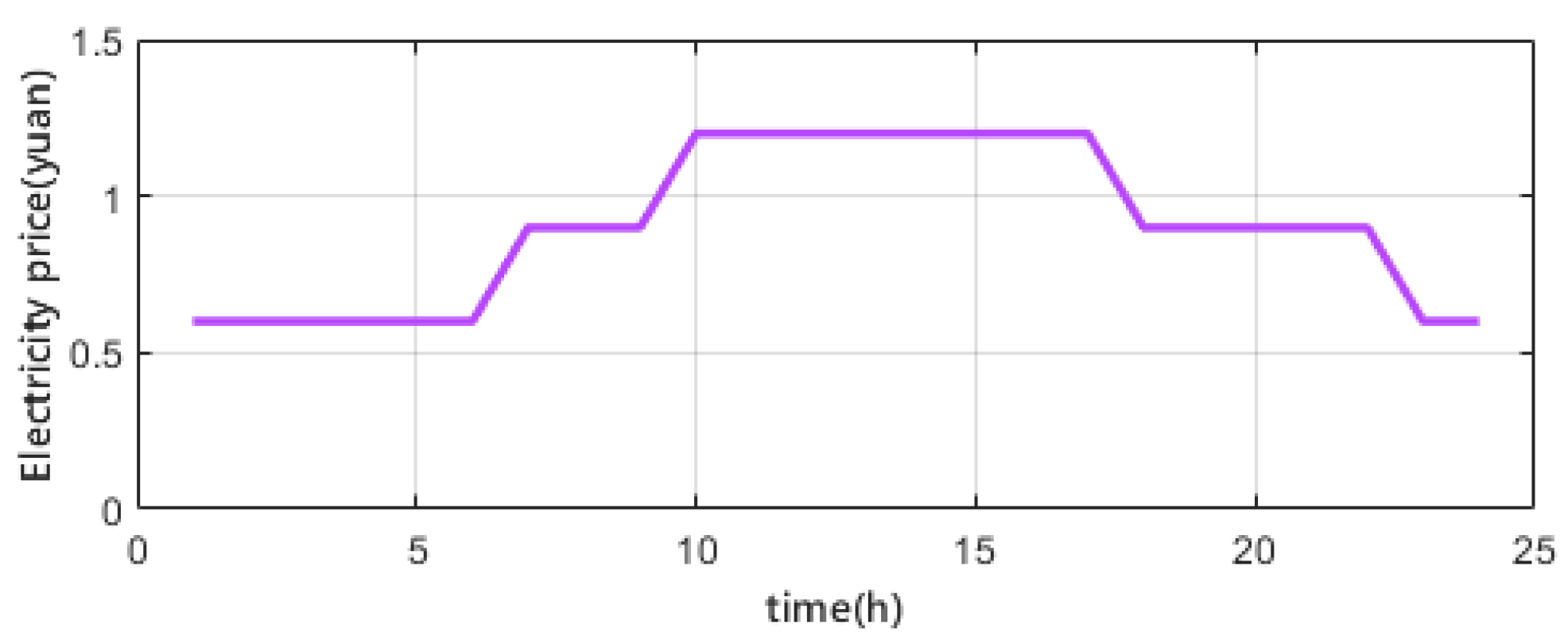
3.1. Data Description and Processing

It is difficult to obtain a complete dataset, and the dataset used in the case study consists of two parts. The data of PV and wind power is retrieved from the China Meteorological Data Service Centre whilst the load data comes from a hotel in the United States. Both data cover a one-year period and the time resolution is one hour. Due to the rich wind resources, meteorological data of the Fujin area in Heilongjiang province of China is selected. The major parameters include directional irradiation HA, wind speed, etc. For the PV generation, polycrystalline silicon components are used with conversion efficiency $K_1$ of 18% and overall efficiency $K_2$ of 90%. In terms of the wind generation, a 600 kW wind turbine S43 supplied by Goldwind is used. The diameter of its blade diameter is 43.2 m and the specified cut-in speed is 3 m/s. Note that the local air density is assumed to be $1.2 \mathrm{kg}/{\mathrm{m}}^3$.

$$P_{PV}=\mathrm{HA}\times \mathrm{S}\times K_1\times K_2$$

(36)

$$P_W=\frac{1}{2}\rho v^{3}S$$

(37)

Using Equations (36) and (37), the actual output of the wind turbine and PV panel can be calculated. Since this study focuses on the day-ahead economic scheduling, the input to the model should be the predicted values. On top of the actual values achieved from Equations (36) and (37), a disturbance that is a function of time t (1.5t/100) is added to construct the input data for the model. Figure 5 shows the input data for the LSTM training set.

The output of the model is the day-ahead economic scheduling scheme for the HPES and for both optimization approaches (i.e., MILP based and CVaR based), the step size is 1 h. The confidence level of CVaR is configured as 0.99 and the number of Monte Carlo simulation is set as 200. The aforementioned optimization process is encoded in YALMIP and solved by CPLEX 12.8.0.

Table 1. Parameters of devices.

Device	Quantity	Parameter	Value
Grid	/	$P_{grid.b}^{max}$	1000
		$P_{grid.s}^{max}$	1000
Electric Boiler	2	${\eta }_{EB}$	0.95
		$Q_{EB}^{max}$	240
Absorption Chiller	12	${\eta }_{AC}$	0.8
		$Q_{AC}^{max}$	50
Hydrogen Storage Tank	5	$V_{H_2}^{max}$	200
		$v_{hst.o}^{max}$	20
		$v_{hst.i}^{max}$	20
Heat Pump	14	$CO{P}_{HP.c}$	3.85
		$CO{P}_{HP.h}$	4
		$Q_{HP.c}^{max}$	38
		$Q_{HP.h}^{max}$	38
Fuel Cell	1	${\delta }_{HFC}$	1
		$v_{H_2.HFC}^{max}$	35
Heat Exchanger	1	${\eta }_{HE}$	0.85
		$Q_{HE.water}^{max}$	150
Electric Refrigerator	6	$CO{P}_{EC}$	4
		$Q_{EC}^{max}$	20
CCHP	1	$v_{ng}^{max}$	200
		$MN$	80
		$P_{CHP}^{max}$	600
		$P_{CHP}^{min}$	60
		$R$	100
Electrolyser	3	${\delta }_{EL}$	5
		$v_{hst.i}^{max}$	50

lists the major parameters of the devices within HPES whilst Figure 6 illustrates the grid electricity price.

3.2. LSTM Network Training Process

Because the data in the input space has obvious seasonal characteristics (as shown in Figure 5), it is determined to involve the first 27 days of each month within the entire 12-month data set as the training set, which is equivalent to 7776 h. The remaining 984-h data is used as the test set. Note that the timestep = 1 h. The LSTM model established in this paper is implemented using the LSTM module of the keras framework that is built upon TensorFlow. In Win10 system, the tests are conducted using the Python-based Spyder environment. The output dimension of the LSTM layer is 100 and a fully connected layer is attached to the LSTM layer. There are 11 neurons in the output layer indicating the predicted values associated with the device operating status at the next time interval. The LSTM network parameters are shown in

Table 2. LSTM Network Parameters.

Parameter	Experiment 1	Experiment 2
Dimension of LSTM Layer Output	100	100
Loss Function	MAE	MAE
Number of Iteration	600	450
Dimension of Output Layer	11	11
Data Set	365	365
Learning Rate	0.001	0.001
Solver	adam	adam

.

3.3. Result Analysis

3.3.1. Analysis of Training Results

Taking the data of 29th June in the test set as an example, the predicted results in Experiment 1 and Experiment 2 are presented in Figure 7 and Figure 8. The dotted lines highlight the results of applying the MILP and CVaR optimization whilst the solid line shows the LSTM predicted results. The optimization results and learning results of the heat pump cooling power are 0 in both Experiment 1 and Experiment 2 and thus are not illustrated in the figures. In Experiment 1, the predicted results are roughly the same as the optimization results and the locations of the crest and trough are similar, but there are certain gaps between the predicted results and optimization results from the perspective of numeral value. In Experiment 2, the trends and values of the predicted results and optimization results are very close. In both experiments, the predicted operation status of the CCHP unit (which is a critical device in the integrated energy system) is correct. It is worth noting that the LSTM is able to facilitate the time series related day-ahead economic scheduling of an integrated energy system.

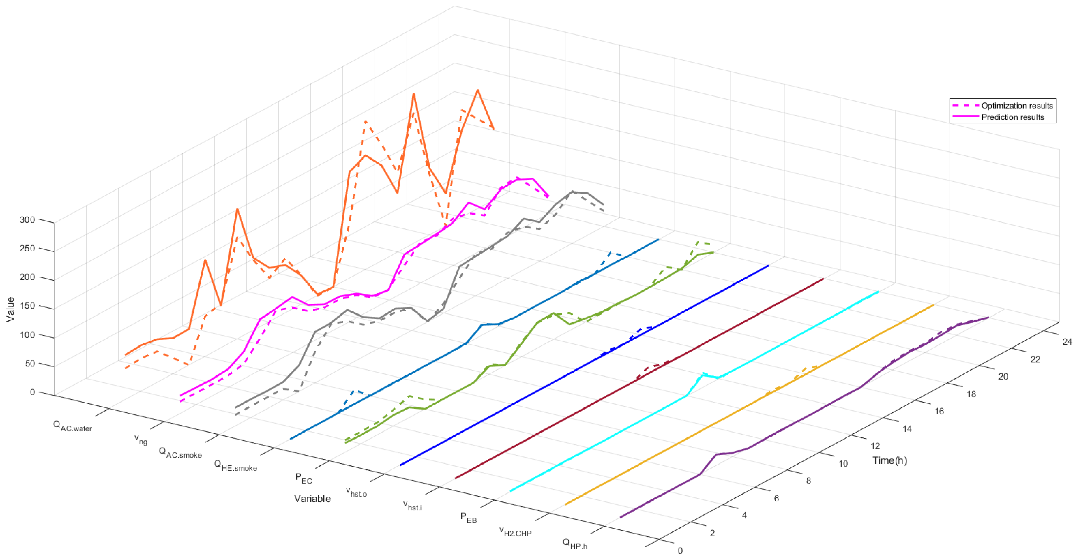
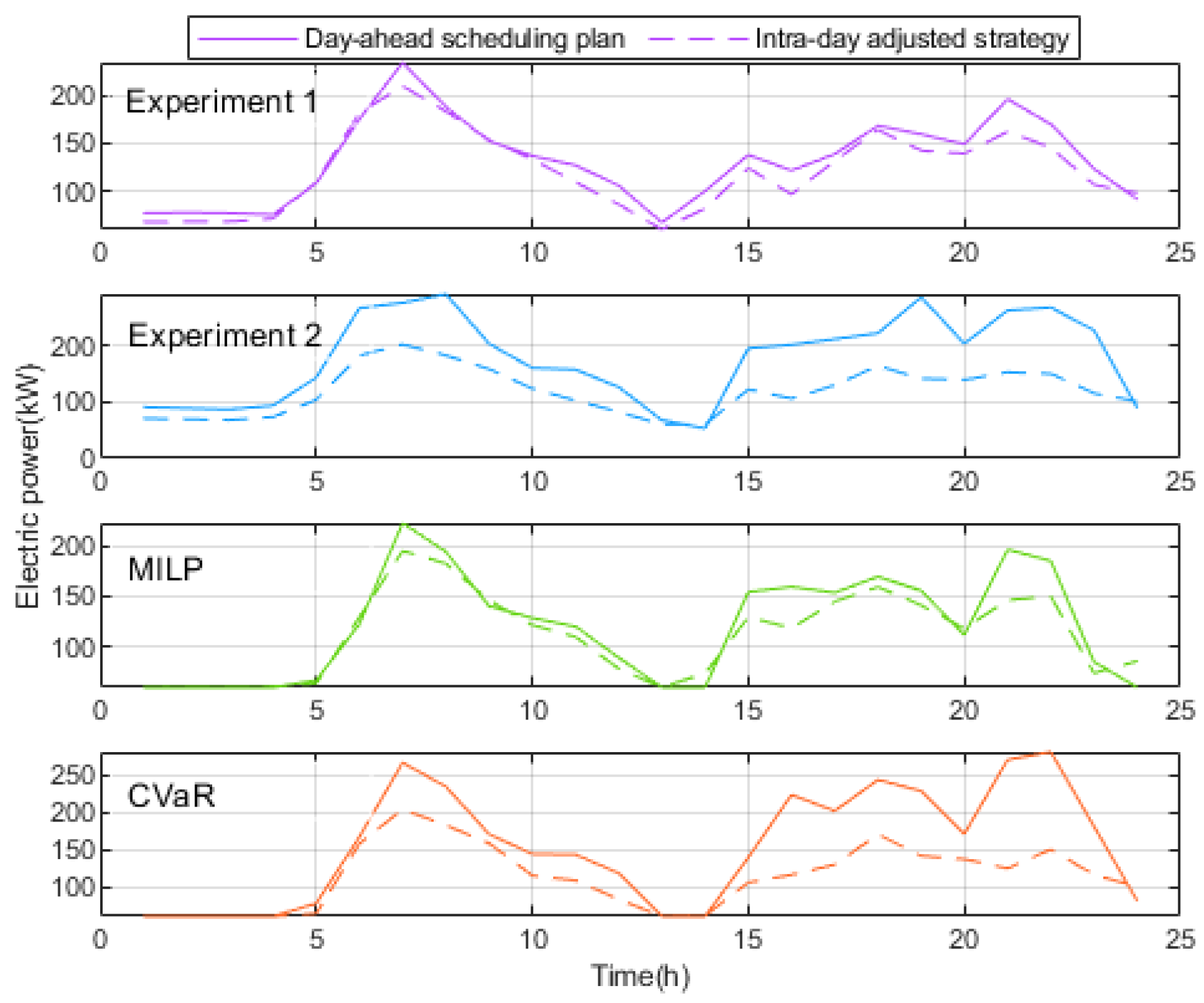
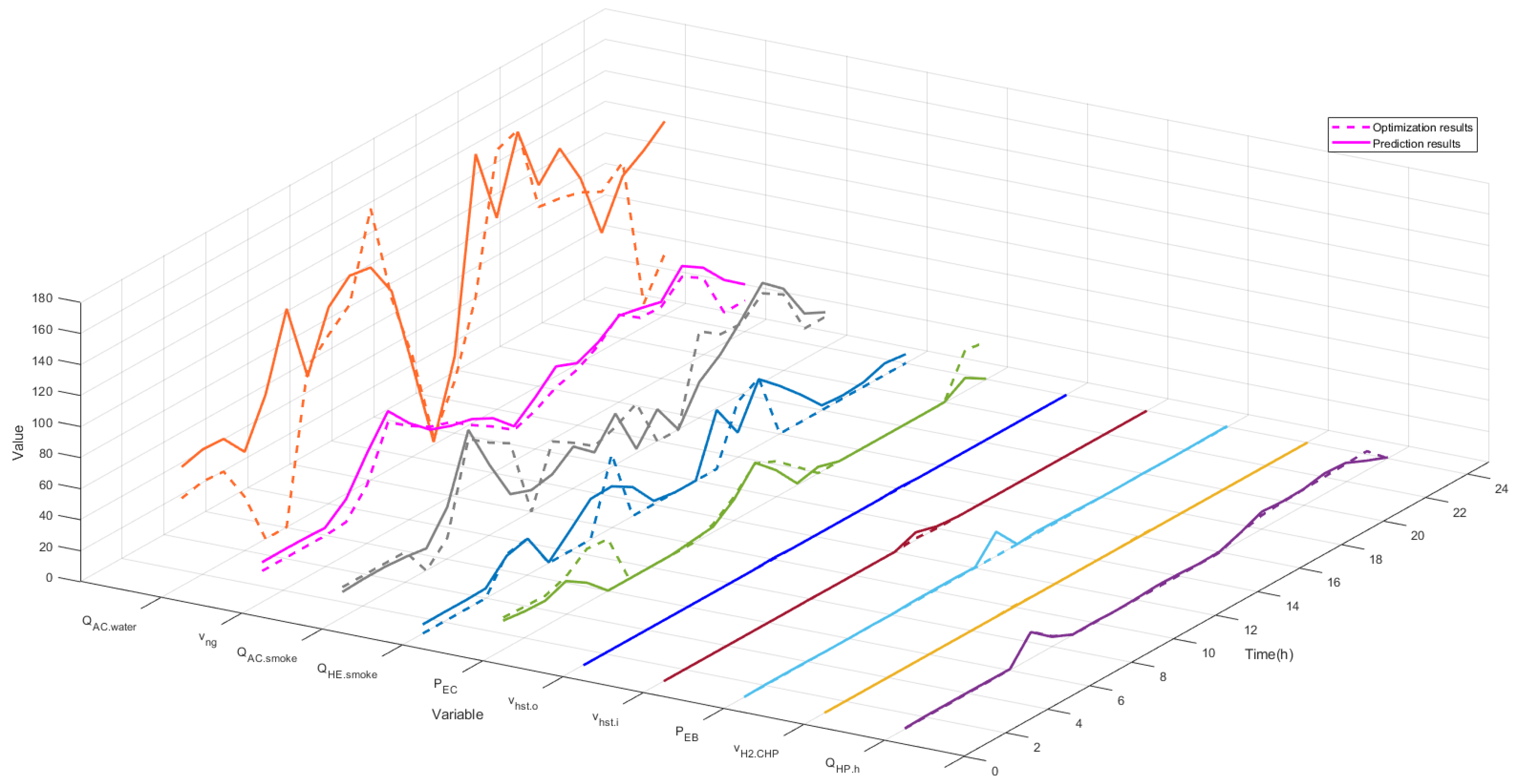
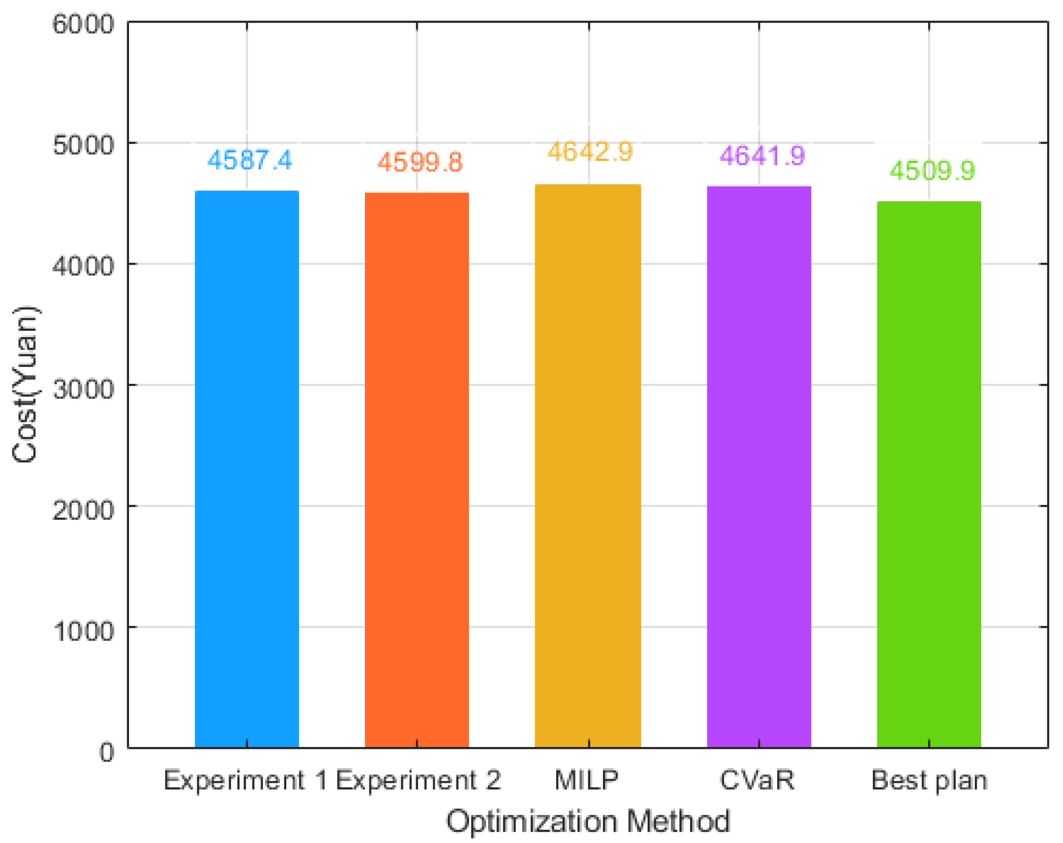
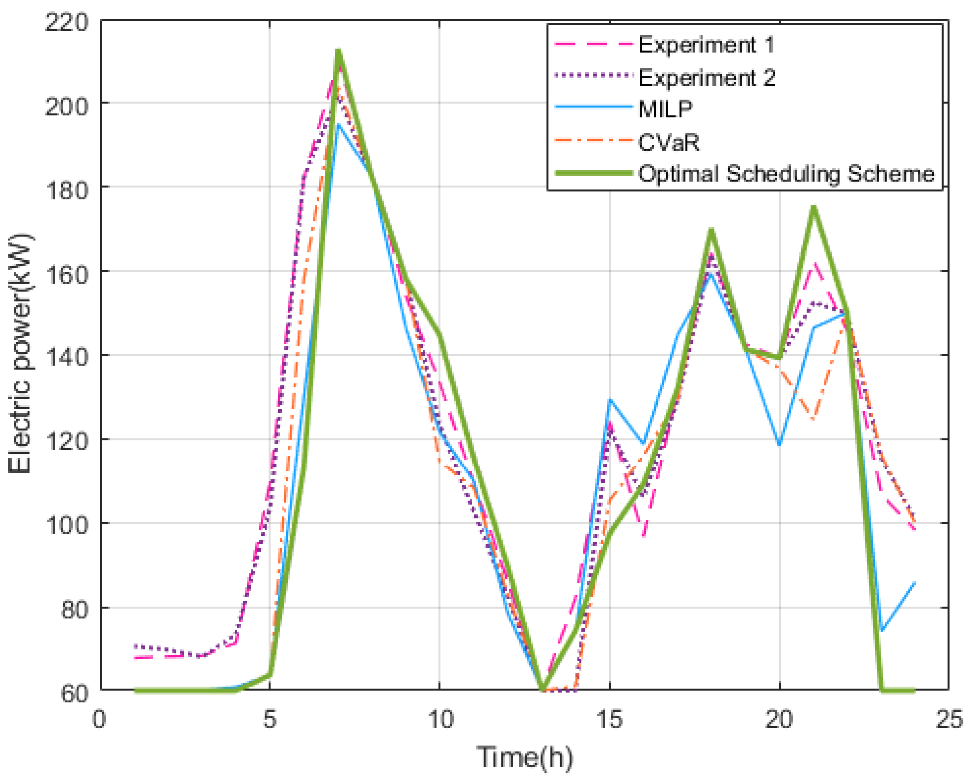
3.3.2. Verification of Training Results on Intra-Day Basis

In order to analyze the training results of Experiment 1 and Experiment 2, an intra-day rolling optimization model is constructed to fine-tune the day-ahead economic scheduling scheme so that the intra-day loading requirement can be satisfied. The step size for the intra-day rolling optimization is 1 h whilst the renewable energy output and load takes the actual values of the day. The rolling period $T$ is 4 h and the optimization aims to minimize the adjustment to the day-ahead scheme. The rolling optimization will be performed for 21 times. In the 1st to 20th optimization, the scheduling scheme of the first period in each optimization attempt is taken as the intra-day scheduling scheme for the HPES whilst the optimization results of the 21st attempt were used as the scheduling scheme for 21 to 24 h within the day.

In each optimization, the day-ahead economic scheduling scheme predicted by LSTM network ${\mathit{O}}_{PRE}$ and the optimized scheduling scheme achieved by applying intra-day rolling optimization ${\mathit{O}}_{INT}$ are both $4\times 11$ matrices. Matrix $\Omega$ is the difference between the two schemes.

$$\Omega ={\mathit{O}}_{PRE}-{\mathit{O}}_{INT}=\left[\begin{array}{c}{\omega }_{1,1}\cdots {\omega }_{1,j}\cdots {\omega }_{1,11}\\ {\omega }_{2,1}\cdots {\omega }_{2,j}\cdots {\omega }_{2,11}\\ {\omega }_{3,1}\cdots {\omega }_{3,j}\cdots {\omega }_{3,11}\\ {\omega }_{4,1}\cdots {\omega }_{4,j}\cdots {\omega }_{4,11}\end{array}\right]$$

(38)

For the intra-day rolling optimization, it is still essential to meet the busbar constraints and device constraints. The objective function during each rolling optimization attempt is given below.

$$\mathrm{Objective}:\min {\displaystyle \sum }_{i=1}^4{\displaystyle \sum }_{j=1}^{11}\left|{\omega }_{i,j}\right|$$

$$\mathrm{Constraints}:\left(1\right)–\left(22\right),\left(38\right)$$

In this section, we will compare the advantages and disadvantages of the four methods from the perspectives of economics, adjustment extent, and electricity purchase.

(a) Economic Analysis

Based on the results of intra-day rolling optimization, the intra-day operating cost of the integrated energy system can be calculated using Equations (23)–(25). In this paper, 41 days’ data within the test set are used in Experiment 1, Experiment 2, MILP optimization and CVaR optimization to determine the day-ahead scheduling schemes. After the intra-day rolling optimization, the corresponding intra-day operating cost is derived. Figure 9 presents the average intra-day operating cost in 41 days for each optimization approach and the best plan. By applying the MILP optimization to the actual data, the optimal intra-day scheduling scheme is achieved. The MILP based method results in the highest average operating cost of ¥4642.9, which is ¥1 higher than that obtained from the CVaR based method. Experiment 1 leads to the lowest average operating cost of ¥4587.4 which is lower than that of MILP by 1.17%. The average cost obtained in Experiment 2 is ¥4599.8 which is lower than that of MILP by 0.93%. The final result of Experiment 1 is closest to the optimal solution. It can be observed that the average intra-day operating costs of Experiment 1 and Experiment 2 are lower than those of MILP and CVaR methods, which proves the feasibility of using LSTM model for day-ahead economic scheduling and the economic performance is better than MILP and CVaR.

(b) Analysis of Adjustment Extent

The extent of adjustment (implemented by the intra-day rolling optimization) to the day-ahead economic scheduling reflects the resistance of the day-ahead operation plan to the uncertainty (PV power, wind power, and load) in the system. This paper uses the CCHP unit (which is a critical device in the integrated energy system) as an example to analyze the performance of four day-ahead optimization methods (i.e., Experiment 1, Experiment 2, MILP, and CVaR) when various uncertainties are seen on predicted values. Figure 10 depicts the extent of adjustment to the day-ahead CCHP electrical power output plan on 29th June, when different optimization methods are used. Considerable adjustment is observed for Experiment 2 and CVaR. The reason is that CVaR produces a relatively conservative optimization strategy in order to deal with the uncertainty of renewable generation and load within the integrated energy system. Since the data set of Experiment 2 is optimized by CVaR, similar adjustment extent is observed. The adjustment of Experiment 1 and MILP is small, even when the uncertainties of the predicted values are significant during 15 h and 24 h. The total amount of adjustment for each optimization method is listed below.

• Experiment 1: 295.5 kWh
• Experiment 2: 1444.7 kWh
• MILP: 326.5 kWh
• CVaR: 1,019 kWh

The adjustment of Experiment 1 is the lowest and only accounts for 20% of that of Experiment 2.

The CCHP operation plan obtained from Experiment 1, Experiment 2, MILP, and CVaR methods is compared to that from the optimal intra-day scheduling scheme as presented in Figure 11. In the first 1–8 h, the predicted values are relatively accurate and thus the optimization strategies provided by MILP and CVaR are closer to the optimal intra-day scheduling scheme. When the error of the predicted values grows, the gaps between the MILP and CVaR strategies and the optimal strategy are more obvious. By contrast, the optimization strategy derived from Experiment 1 maintains close to the optimal scheme in the later period, outperforming the other three strategies. This can also be verified by the associated system operation cost where Experiment 1 sees the lowest cost of ¥5493. The system operation cost of Experiment 2, MILP and CVaR are ¥5504.3, ¥5653.6 and ¥5548.4, respectively.

(c) Analysis of Electricity Purchase

This section compares the amount of electricity that is required to be purchased when using different intra-day rolling scheduling schemes and Figure 12 shows the results on 29th June. The amount of the purchased electricity in Experiment 1 is 3232.2 kWh which is the smallest among all four optimization schemes. It is lower than that of Experiment 2, MILP and CVaR by 1.6%, 13.4%, and 8.5%, respectively. Purchasing less mount of electricity can reduce the grid pressure and Experiment is superior to other methods from this perspective.

3.3.3. Running Time of Optimization Program

Table 3. Comparison of Optimization Program Running Time.

Optimization Method	Experiment 1	Experiment 2	MILP	CVaR
Time(s)	0.16	0.23	0.98	586.5

compares the difference of the optimization running time when applying the four methods to the data of 29th June. All optimization programs are run on a Windows 10 computer with Intel Core i7 8750H 2.2 GHz CPU and 16 GB 2666 MHz memory. The LSTM model takes the least amount of time around 0.2 s whilst MILP requires 0.98 s. The running time of CVaR is approximately 3000 times of the LSTM running time.

4. Conclusions

In order to explore the advantages and disadvantages of traditional optimization methods such as MILP and CVaR and the emerging machine learning methods for day-ahead economic scheduling of integrated energy systems, this paper proposes an LSTM model that can learn the optimized results achieved by applying the MILP and CVaR optimization methods and analyses the accuracy of the learning results. The objective function is specified so that the intra-day rolling optimization with the smallest deviation from the day-ahead scheduling scheme can be achieved. Based on such objective functions, the day-ahead economic scheduling scheme provided by Experiment 1, Experiment 2, MILP, and CVaR are compared in terms of economy, adjustment to achieve intra-day rolling optimization, the total amount of purchased electricity, and optimization running speed. From this, several conclusions can be made.

Experiment 1 and Experiment 2 use the LSTM model to learn the optimization results obtained from MILP and CVaR, respectively. According to the training results, the LSTM predicted values are close to the optimization results of the test set in terms of the time dimension and device operating trend. This proves the feasibility of using the LSTM model for the day-ahead economic scheduling of an integrated energy system.

Subsequently, the training results obtained from Experiment 1 and Experiment 2 are optimized for the intra-day rolling and compared with those obtained via using MILP and CVaR optimization methods. Among the four optimization methods, Experiment 1 leads to the lowest average operating cost and the smallest adjustment of CCHP for intra-day scheduling. The associated intra-day scheduling after applying the adjustment is also the closest to the optimal scheduling scheme-based optimization on actual data. In the interaction with the grid, the purchase of electricity in Experiment 1 also has the least amount of purchased electricity. This proves that the LSTM is superior to the MILP and CVaR for the day-ahead economic scheduling of integrated energy systems.

Experiment 1 and Experiment 2 are faster than MILP and CVaR. Considering the training results and the intra-day rolling optimization results, Experiment 1 (i.e., LSTM model is used to learn the results that are obtained by applying MILP optimization to the actual historical data) outperforms the Experiment 2, MILP, and CVaR, and can be used for the day-ahead economic scheduling of HPES.

This paper verifies the performance of LSTM in the economic dispatching of hydrogen-containing energy systems, but the types of equipment in the system are not enough, and the performance of LSTM in the process of intraday rolling optimization and real-time optimization scheduling is not examined. The application of LSTM in the daytime rolling optimization and real-time optimization scheduling will become the focus of the next step, and more energy conversion equipment will be added to the system structure.

References

1. Mancarella, P. MES (multi-energy systems): An overview of concepts and evaluation models. Energy 2014, 65, 1–17. [Google Scholar] [CrossRef]
2. Bitar, E.; Khargonekar, P.P.; Poolla, K. Systems and control opportunities in the integration of renewable energy into the smart grid. IFAC Proc. Vol. 2011, 44, 4927–4932. [Google Scholar] [CrossRef]
3. Korpås, M.; Greiner, C.J. Opportunities for hydrogen production in connection with wind power in weak grids. Renew. Energy 2008, 33, 1199–1208. [Google Scholar] [CrossRef]
4. Hajimiragha, A.; Canizares, C.; Fowler, M.; Geidl, M.; Andersson, G. Optimal energy flow of integrated energy systems with hydrogen economy considerations. In Proceedings of the 2007 iREP Symposium-Bulk Power System Dynamics and Control-VII. Revitalizing Operational Reliability, Charleston, SC, USA, 19–24 August 2007; pp. 1–11. [Google Scholar]
5. Winter, C.-J.; Nitsch, J. Hydrogen as an Energy Carrier: Technologies, Systems, Economy; Springer Science & Business Media: Berlin, Germany, 2012. [Google Scholar]
6. Zhou, S.; He, D.; Gu, W.; Wu, Z.; Abbas, G.; Hong, Q.; Booth, C. Design and evaluation of operational scheduling approaches for HCNG penetrated integrated energy system. IEEE Access 2019, 7, 87792–87807. [Google Scholar] [CrossRef]
7. De Santoli, L.; Basso, G.L.; Bruschi, D. Energy characterization of CHP (combined heat and power) fuelled with hydrogen enriched natural gas blends. Energy 2013, 60, 13–22. [Google Scholar] [CrossRef]
8. Wu, Q.; Zheng, J.; Jing, Z. Coordinated scheduling of energy resources for distributed DHCs in an integrated energy grid. CSEE J. Power Energy Syst. 2015, 1, 95–103. [Google Scholar] [CrossRef]
9. Sugihara, H.; Komoto, J.; Tsuji, K. A multi-objective optimization model for determining urban energy systems under integrated energy service in a specific area. Electr. Eng. Jpn. 2004, 147, 20–31. [Google Scholar] [CrossRef]
10. Geidl, M. Integrated Modeling and Optimization of Multi-Carrier Energy Systems; ETH Zurich: Zurich, Switzerland, 2007. [Google Scholar]
11. Sanjari, M.; Karami, H.; Gooi, H. Micro-generation dispatch in a smart residential multi-carrier energy system considering demand forecast error. Energy Convers. Manag. 2016, 120, 90–99. [Google Scholar] [CrossRef]
12. Ma, H.; Wang, B.; Gao, W.; Liu, D.; Sun, Y.; Liu, Z. Optimal scheduling of a regional integrated energy system with energy storage systems for service regulation. Energies 2018, 11, 195. [Google Scholar] [CrossRef]
13. Tan, Z.; Ju, L.; Li, H.; Qin, C.; Peng, D. Multiobjective CVaR optimization model and solving method for hydrothermal system considering uncertain load demand. Math. Probl. Eng. 2015, 2015, 741379. [Google Scholar] [CrossRef]
14. Li, G.; Zhang, R.; Jiang, T.; Chen, H.; Bai, L.; Li, X. Security-constrained bi-level economic dispatch model for integrated natural gas and electricity systems considering wind power and power-to-gas process. Appl. Energy 2017, 194, 696–704. [Google Scholar] [CrossRef]
15. Ahmadi, P.; Dincer, I.; Rosen, M.A. Thermoeconomic multi-objective optimization of a novel biomass-based integrated energy system. Energy 2014, 68, 958–970. [Google Scholar] [CrossRef]
16. Jiang, X.; Jing, Z.; Li, Y.; Wu, Q.; Tang, W. Modelling and operation optimization of an integrated energy based direct district water-heating system. Energy 2014, 64, 375–388. [Google Scholar] [CrossRef]
17. Firestone, R.; Stadler, M.; Marnay, C. Integrated energy system dispatch optimization. In Proceedings of the 2006 4th IEEE International Conference on Industrial Informatics, Singapore, 16–18 August 2006; pp. 357–362. [Google Scholar]
18. Martinez-Mares, A.; Fuerte-Esquivel, C.R. A robust optimization approach for the interdependency analysis of integrated energy systems considering wind power uncertainty. IEEE Trans. Power Syst. 2013, 28, 3964–3976. [Google Scholar] [CrossRef]
19. Costanzo, G.T.; Iacovella, S.; Ruelens, F.; Leurs, T.; Claessens, B.J. Experimental analysis of data-driven control for a building heating system. Sustain. Energy Grids Netw. 2016, 6, 81–90. [Google Scholar] [CrossRef]
20. Smarra, F.; Jain, A.; de Rubeis, T.; Ambrosini, D.; D’Innocenzo, A.; Mangharam, R. Data-driven model predictive control using random forests for building energy optimization and climate control. Appl. Energy 2018, 226, 1252–1272. [Google Scholar] [CrossRef]
21. Darivianakis, G.; Georghiou, A.; Smith, R.S.; Lygeros, J. The power of diversity: Data-driven robust predictive control for energy-efficient buildings and districts. IEEE Trans. Control Syst. Technol. 2017, 27, 132–145. [Google Scholar] [CrossRef]
22. Zhou, S.; Wu, Z.; Gu, W. Potential of Model-Free Control for Demand-Side Management Considering Real-Time Pricing. Energies 2019, 12, 2587. [Google Scholar] [CrossRef]
23. Zhou, S.; Hu, Z.; Gu, W.; Jiang, M.; Zhang, X.-P. Artificial intelligence based smart energy community management: A reinforcement learning approach. CSEE J. Power Energy Syst. 2019, 5, 1–10. [Google Scholar] [CrossRef]
24. Qin, Z.; Xifan, W. Hedge contract characterization and risk-constrained electricity procurement. IEEE Trans. Power Syst. 2009, 24, 1547–1558. [Google Scholar]
25. Hochreiter, S.; Schmidhuber, J. Long short-term memory. Neural Comput. 1997, 9, 1735–1780. [Google Scholar] [CrossRef] [PubMed]
Figure 1. Structure of the hydrogen penetrated energy system (HPES).
Sustainability 11 06784 g001
Figure 2. Data-driven approach for HPES scheduling.
Sustainability 11 06784 g002
Figure 3. Network structure of Long Short-Term Memory (LSTM).
Sustainability 11 06784 g003
Figure 4. Internal architecture of an LSTM unit.
Sustainability 11 06784 g004
Figure 5. Input data for the LSTM training set.
Sustainability 11 06784 g005
Figure 6. Grid Electricity Price.
Sustainability 11 06784 g006
Figure 7. Predicted results of 29th June in Experiment 1.
Sustainability 11 06784 g007
Figure 8. Predicted results of 29th June in Experiment 2.
Sustainability 11 06784 g008
Figure 9. Average intra-day operating cost using various optimization methods.
Sustainability 11 06784 g009
Figure 10. Comparison of adjustment to the day-ahead combined cooling and heating plant (CCHP) electrical power output plan on 29th June.
Sustainability 11 06784 g010
Figure 11. Comparison of adjustment to the day-ahead CCHP electrical power output plan on 29th June.
Sustainability 11 06784 g011
Figure 12. Comparison of Total Amount of Purchased Electricity on 29th June.
Sustainability 11 06784 g012