Terrestrial Water Storage in China: Spatiotemporal Pattern and Driving Factors


Abstract
1. Introduction
2. Materials
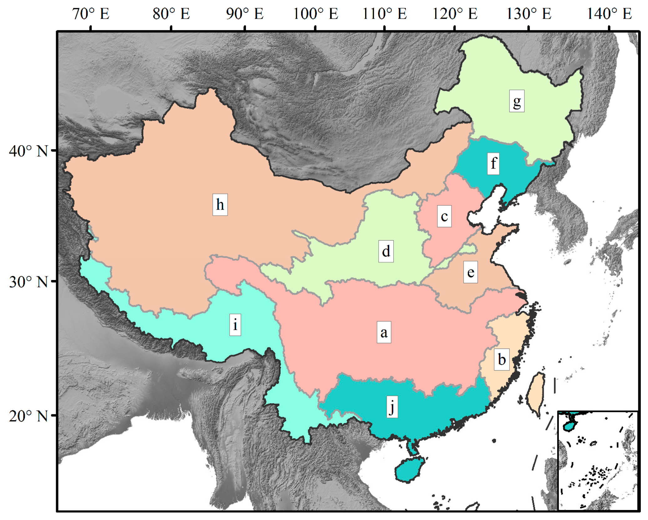
2.1. Study Region
2.2. GRACE Data
2.3. Precipitation Data
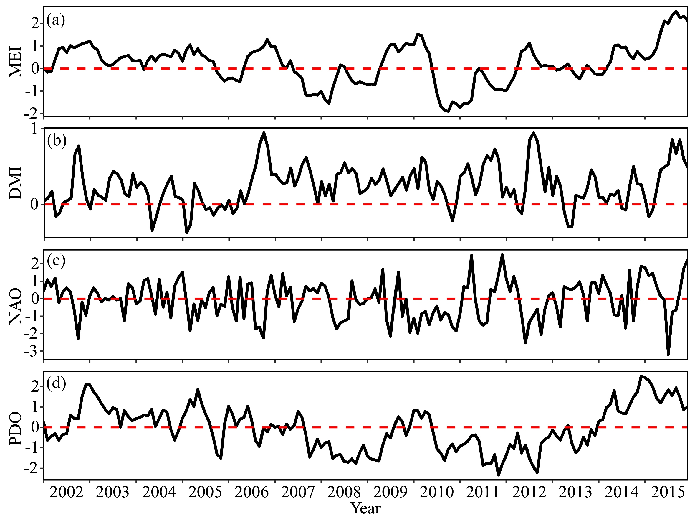
2.4. Climate Index Data
3. Methods
3.1. Seasonal Decomposition of Time Series by LOESS
3.2. Statistical Methods
3.2.1. Linear Regression
3.2.2. Spatial and Temporal Variability
3.2.3. Cross-correlation Analysis
4. Results and Discussion
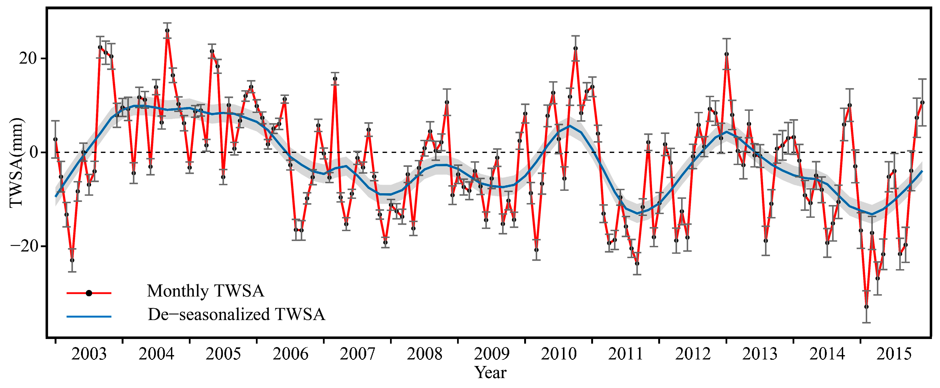
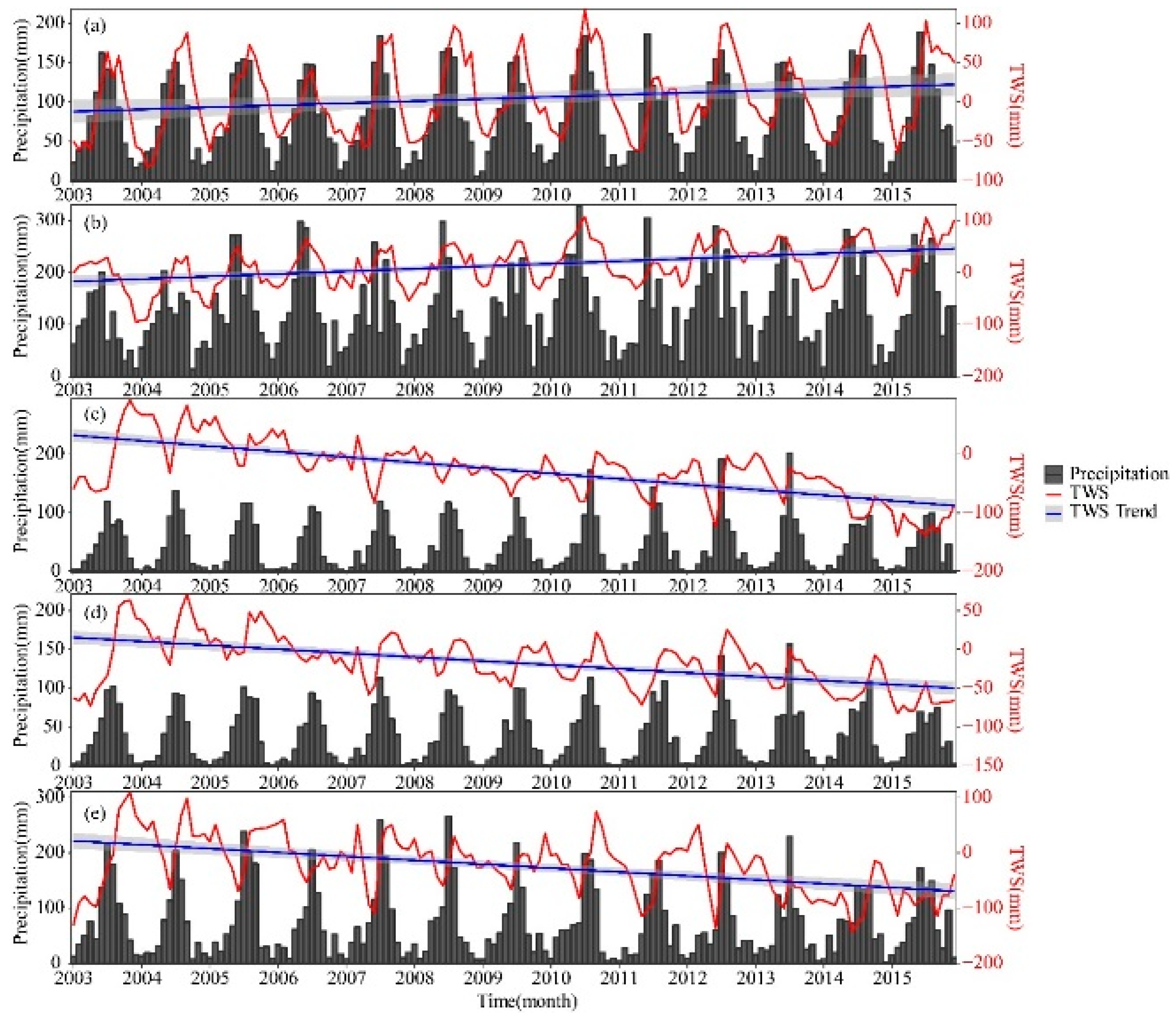
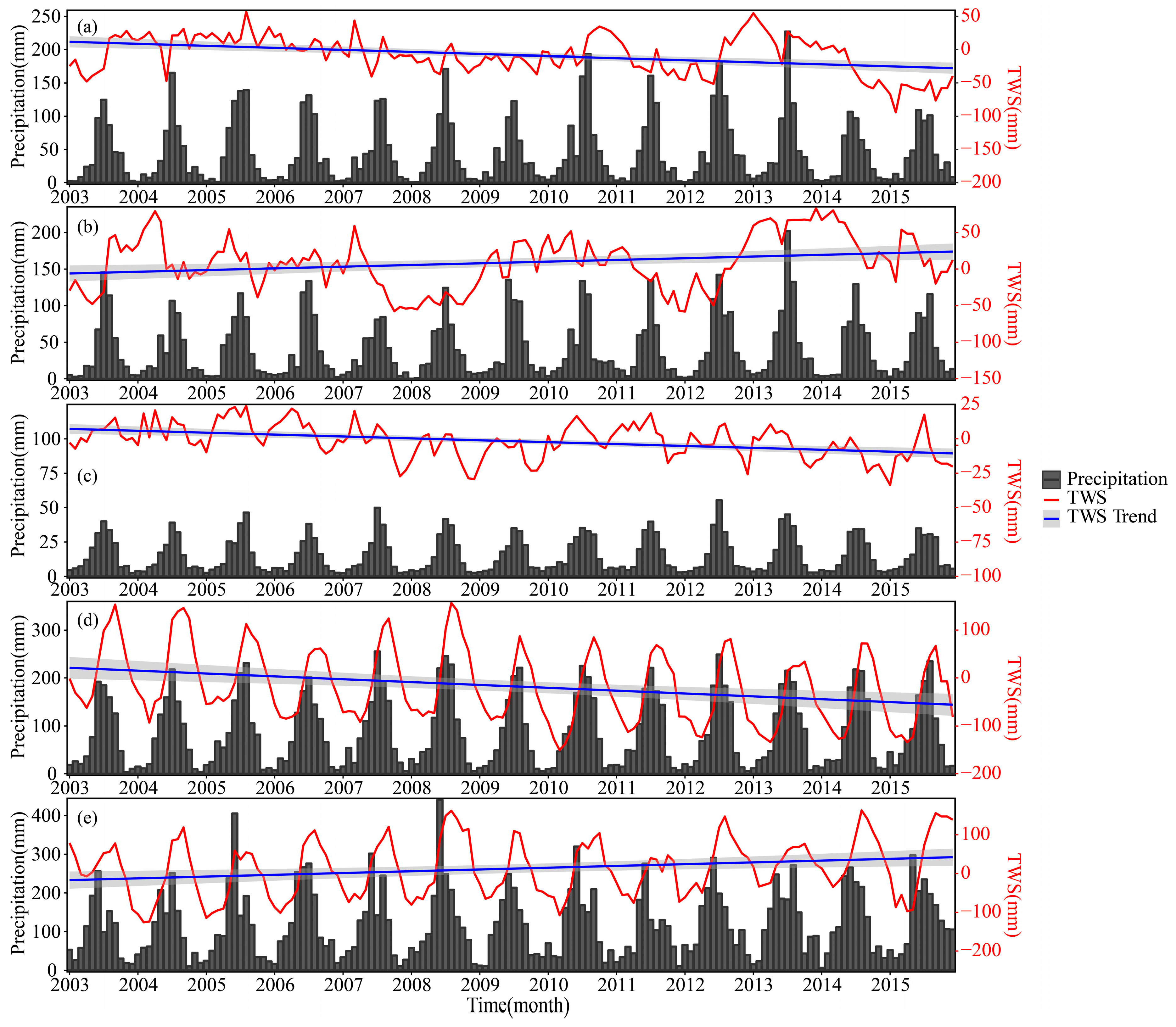
4.1. Temporal Variation Characteristics of the TWS across China
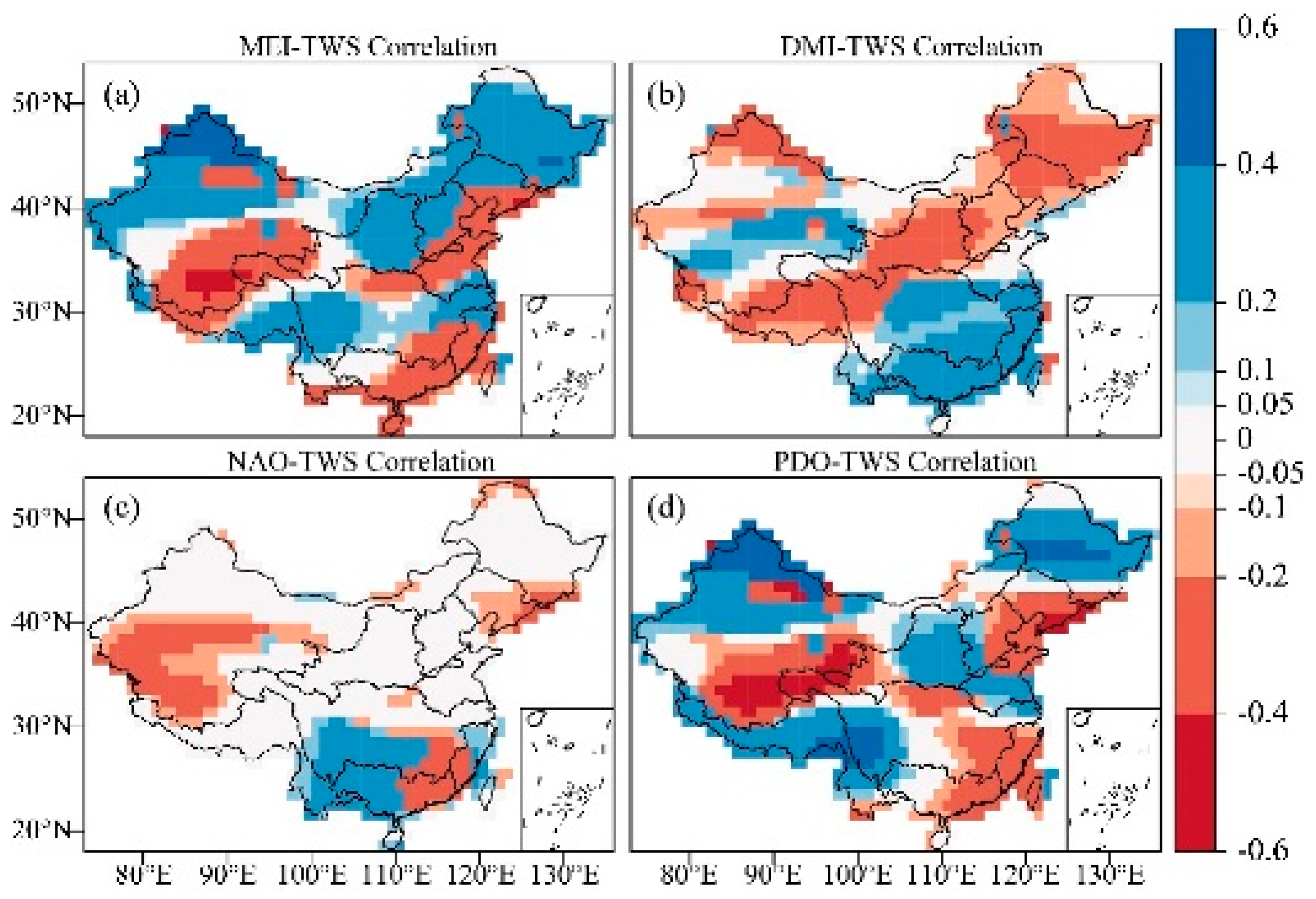
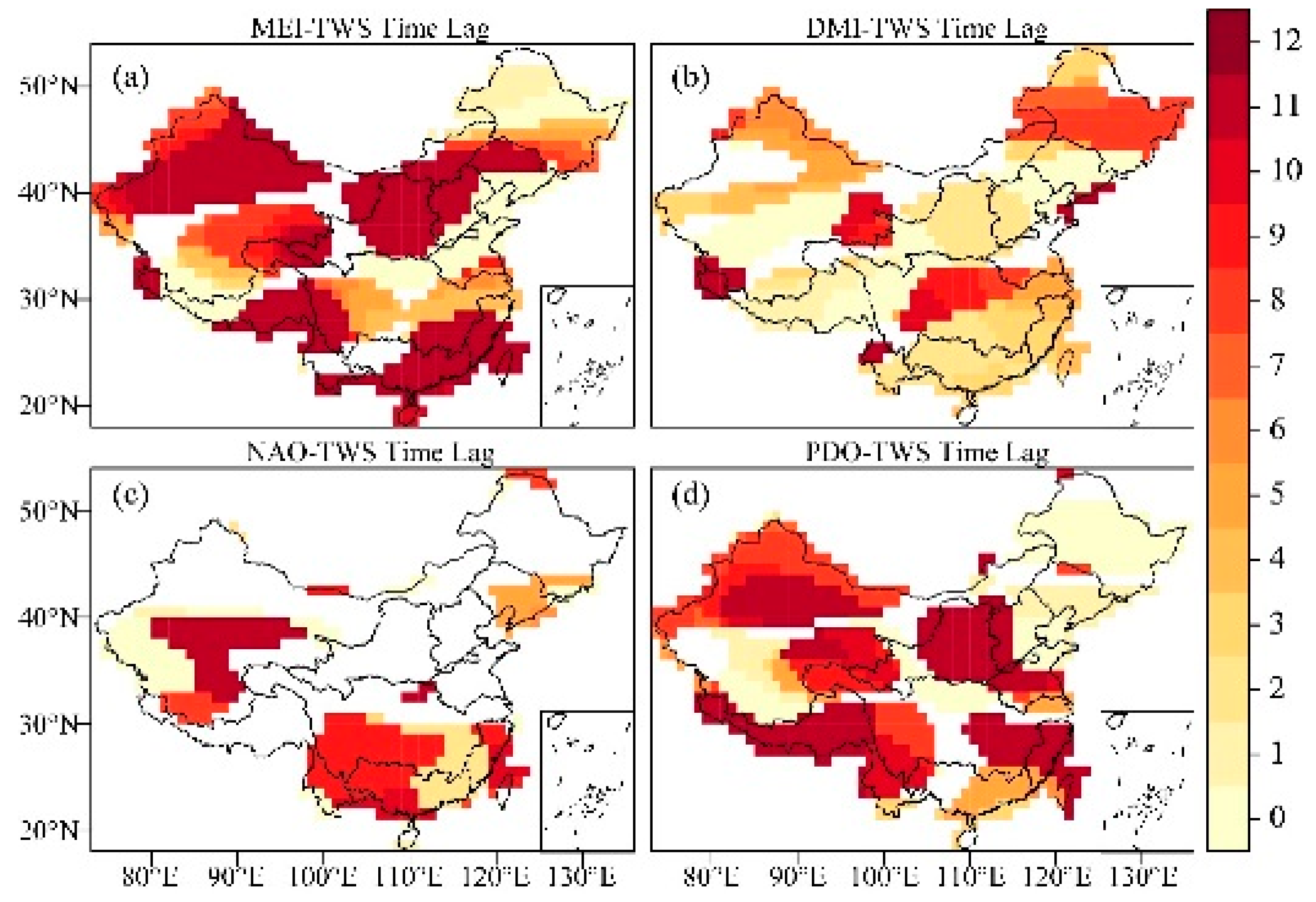
4.2. Cross-Correlations of Climate Modes and TWS
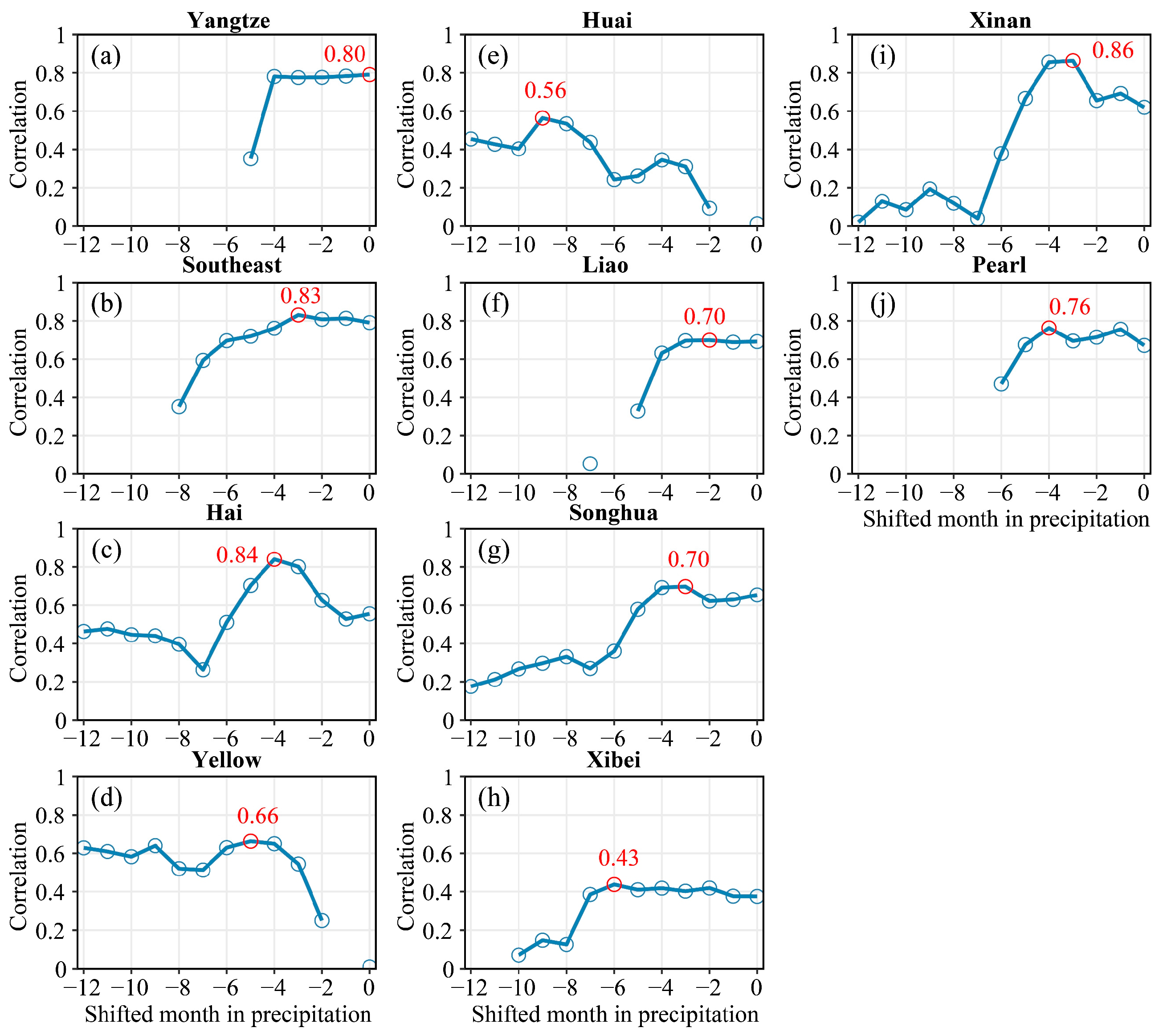
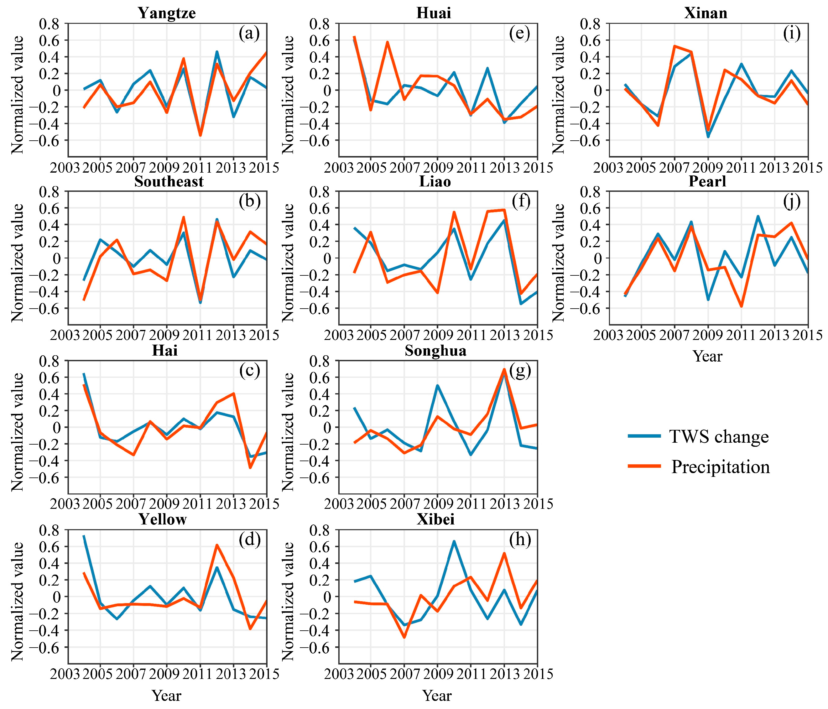
4.3. Relations between Precipitation and TWS
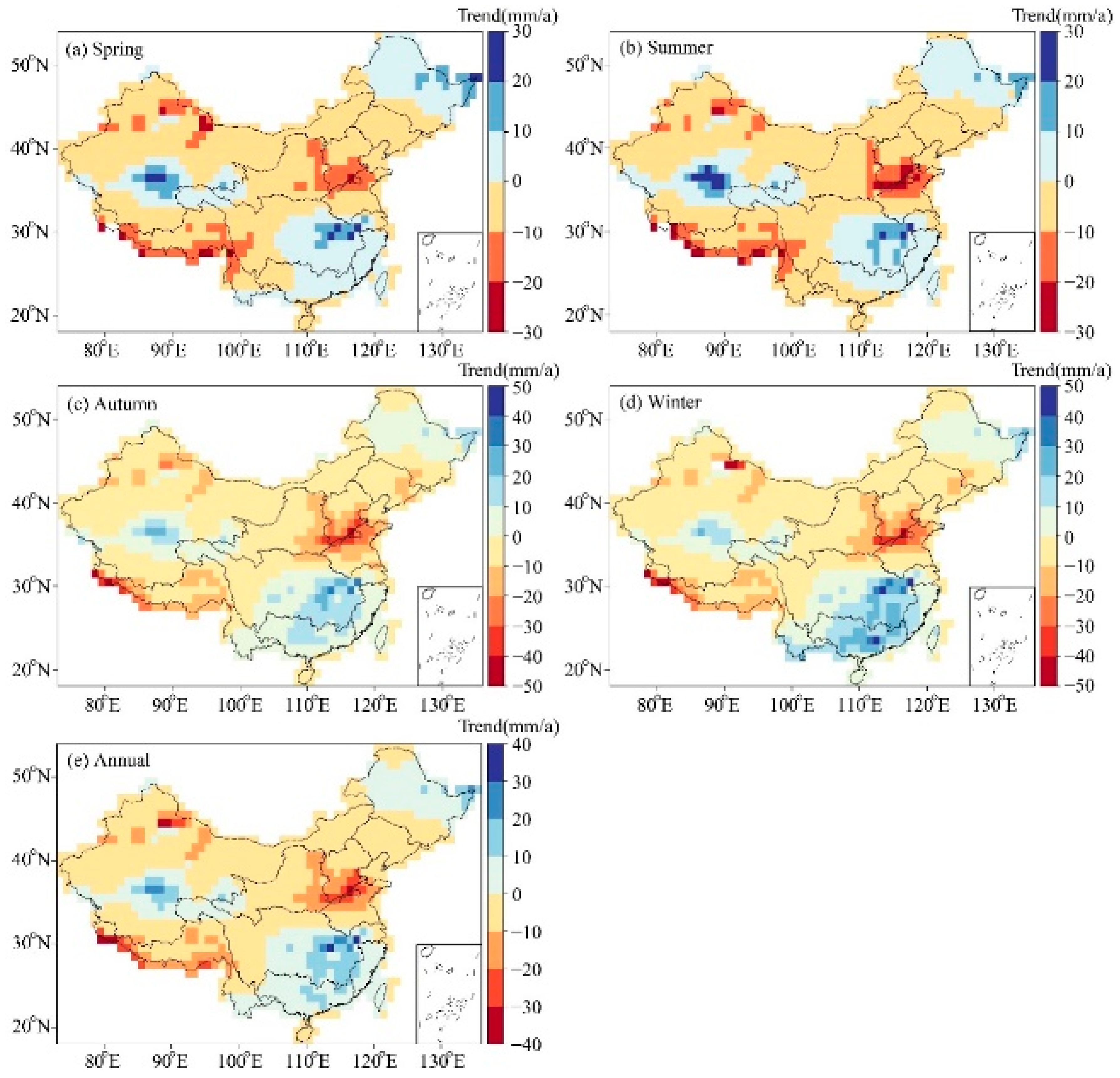
4.4. Spatial Distribution of the TWS Trends at Seasonal and Annual Scale
4.5. Influences of Climate Modes and Precipitation to Variations of TWS
5. Conclusions
Author Contributions
Funding
Conflicts of Interest
References
- Oki, T.; Kanae, S. Global hydrological cycle and world water resources. Science 2006, 313, 1068–1072. [Google Scholar] [CrossRef] [PubMed]
- Zhang, Q.; Li, J.; Singh, V.P.; Xiao, M. Spatio-temporal relations between temperature and precipitation regimes: Implications for temperature-induced changes in the hydrological cycle. Glob. Planet Chang. 2013, 111, 57–76. [Google Scholar] [CrossRef]
- Famiglietti, J.S.; Rodell, M. Water in the balance. Science 2013, 340, 1300–1301. [Google Scholar] [CrossRef] [PubMed]
- Easterling, D.R.; Meehl, G.A.; Parmesan, C.; Changnon, S.A.; Karl, T.R.; Mearns, L.O. Climate extremes: Observations, modeling, and impacts. Science 2000, 289, 2068–2074. [Google Scholar] [CrossRef]
- Chou, C.; Chiang, J.C.; Lan, C.-W.; Chung, C.-H.; Liao, Y.-C.; Lee, C.-J. Increase in the range between wet and dry season precipitation. Nat. Geosci. 2013, 6, 263–267. [Google Scholar] [CrossRef]
- Cai, W.; Borlace, S.; Lengaigne, M.; Van Rensch, P.; Collins, M.; Vecchi, G.; Wu, L. Increasing frequency of extreme El Niño events due to greenhouse warming. Nat. Clim. Chang. 2014, 4, 111–116. [Google Scholar] [CrossRef]
- Briffa, K.R.; Van Der Schrier, G.; Jones, P.D. Wet and dry summers in Europe since 1750: Evidence of increasing drought. Int. J. Climatol. 2009, 29, 1894–1905. [Google Scholar] [CrossRef]
- Cai, W.; Cowan, T.; Briggs, P.; Raupach, M. Rising temperature depletes soil moisture and exacerbates severe drought conditions across southeast Australia. Geophys. Res. Lett. 2009, 36, L21709. [Google Scholar] [CrossRef]
- Wang, J.; Chen, F.; Jin, L.; Bai, H. Characteristics of the dry/wet trend over arid central Asia over the past 100 years. Clim. Res. 2010, 41, 51–59. [Google Scholar] [CrossRef]
- Sheffield, J.; Wood, E.F. Projected changes in drought occurrence under future global warming from multi-model, multi-scenario, IPCC AR4 simulations. Clim. Res. 2008, 31, 79–105. [Google Scholar] [CrossRef]
- Sheffield, J.; Wood, E.F.; Roderick, M.L. Little change in global drought over the past 60 years. Nature 2012, 491, 435–438. [Google Scholar] [CrossRef] [PubMed]
- Hu, P.; Zhang, Q.; Shi, P.; Chen, B.; Fang, J.; Sun, P. Flood-induced mortality across the globe: Spatiotemporal pattern and influencing factors. Sci. Total Environ. 2018, 22, 2637–2653. [Google Scholar] [CrossRef]
- Held, I.M.; Soden, B.J. Robust responses of the hydrological cycle to global warming. J. Clim. 2006, 19, 5686–5699. [Google Scholar] [CrossRef]
- Chou, C.; Tu, J.-Y.; Tan, P.-H. Asymmetry of tropical precipitation change under global warming. Geophys. Res. Lett. 2007, 34, L17708. [Google Scholar] [CrossRef]
- Emori, S.; Brown, S.J. Dynamic and thermodynamic changes in mean and extreme precipitation under changed climate. Geophys. Res. Lett. 2005, 32, L17706. [Google Scholar] [CrossRef]
- Chou, C.; Neelin, J.D.; Chen, C.-A.; Tu, J.-Y. Evaluating the rich-get-richer mechanism in tropical precipitation change under global warming. J. Clim. 2009, 22, 1982–2005. [Google Scholar] [CrossRef]
- Tiwari, V.M.; Wahr, J.; Swenson, S. Dwindling groundwater resources in northern India, from satellite gravity observations. Geophys. Res. Lett. 2009, 36, L18401. [Google Scholar] [CrossRef]
- Scanlon, B.R.; Faunt, C.C.; Longuevergne, L.; Reedy, R.C.; Alley, W.M.; McGuire, V.L.; McMahon, P.B. Groundwater depletion and sustainability of irrigation in the US High Plains and Central Valley. Proc. Natl. Acad. Sci. USA 2012, 109, 9320–9325. [Google Scholar] [CrossRef]
- Voss, K.A.; Famiglietti, J.S.; Lo, M.; Linage, C.; Rodell, M.; Swenson, S.C. Groundwater depletion in the Middle East from GRACE with implications for transboundary water management in the Tigris-Euphrates-Western Iran region. Water Resour. Res. 2013, 49, 904–914. [Google Scholar] [CrossRef]
- Gu, X.; Zhang, Q.; Li, J.; Singh, V.P.; Liu, J.; Sun, P.; Cheng, C. Attribution of global soil moisture drying to human activities: A quantitative viewpoint. Geophys. Res. Lett. 2019, 46, 2573–2582. [Google Scholar] [CrossRef]
- Zhou, L.-T.; Tam, C.-Y.; Zhou, W.; Chan, J.C.L. Influence of South China Sea SST and the ENSO on winter rainfall over South China. Adv. Atmos. Sci. 2010, 27, 832–844. [Google Scholar] [CrossRef]
- Jones, P.D. The influence of ENSO on global temperatures. Clim. Monit. 1988, 17, 80–89. [Google Scholar]
- Kiladis, G.N.; Diaz, H. Global climatic anomalies associated with extremes in the Southern Oscillation. J. Clim. 1989, 2, 1069–1090. [Google Scholar] [CrossRef]
- Huang, R.H.; Zhou, L.T.; Chen, W. The progresses of recent studies on the variabilities of the East Asian monsoon and their causes. Adv. Atmos. Sci. 2003, 20, 55–69. [Google Scholar] [CrossRef]
- Luo, M.; Leung, Y.; Graf, H.-F.; Herzog, M.; Zhang, W. Interannual variability of the onset of the South China Sea summer monsoon. Int. J. Climatol. 2016, 36, 550–562. [Google Scholar] [CrossRef]
- Luo, M.; Lau, N.-C. Heat waves in southern China: Synoptic behavior, long-term change and urbanization effects. J. Clim. 2017, 30, 703–720. [Google Scholar] [CrossRef]
- Wu, R.; Hu, Z.Z.; Kirtman, B.P. Evolution of ENSO-related rainfall anomalies in East Asia and the processes. J. Clim. 2003, 16, 3741–3757. [Google Scholar] [CrossRef]
- Xiao, M.; Zhang, Q.; Singh, V.P. Influences of ENSO, NAO, IOD and PDO on seasonal precipitation regimes in the Yangtze River basin, China. Int. J. Climatol. 2015, 35, 3556–3567. [Google Scholar] [CrossRef]
- Zhang, Q.; Li, J.; Singh, V.P.; Xu, C.-Y.; Deng, J. Influence of ENSO on precipitation in the East River basin, South China. J. Geophys. Res. Atmos. 2013, 118, 2207–2219. [Google Scholar] [CrossRef]
- Zhang, Q.; Wang, Y.; Singh, V.P.; Gu, X.; Kong, D. Impacts of ENSO and ENSO Modoki + A regimes on seasonal precipitation variations and possible underlying causes in the Huai River basin, China. J. Hydrol. 2016, 533, 308–319. [Google Scholar] [CrossRef]
- Zhou, L.T.; Wu, R. Respective impacts of East Asian winter monsoon and ENSO on winter rainfall in China. J. Geophys. Res. Atmos. 2010, 115, D02107. [Google Scholar] [CrossRef]
- Jiang, T.; Zhang, Q.; Zhu, D.M.; Wu, Y.J. Yangtze floods and droughts (China) and teleconnections with ENSO activities (1470–2003). Quatern. Int. 2006, 144, 29–37. [Google Scholar]
- Luo, M.; Lau, N.-C. Amplifying effect of ENSO on heat waves in China. Clim. Dyn. 2019, 52, 3277–3289. [Google Scholar] [CrossRef]
- Wallace, J.M.; Thompson, D.W.J. The Pacific center of action of the Northern Hemisphere annular mode: Real or artifact? J. Clim. 2002, 15, 1987–1991. [Google Scholar] [CrossRef][Green Version]
- Webster, P.J.; Moore, A.M.; Loschnigg, J.P.; Leben, R.R. Coupled ocean-atmosphere dynamics in the Indian Ocean during 1997–98. Nature 1999, 401, 356–360. [Google Scholar] [CrossRef] [PubMed]
- Yuan, Y.; Yang, H.; Zhou, W.; Li, C.Y. Influences of the Indian Ocean dipole on the Asian summer monsoon in the following year. Int. J. Climatol. 2008, 28, 1849–1859. [Google Scholar] [CrossRef]
- Linderholm, H.W.; Ou, T.H.; Jeong, J.H.; Folland, C.K.; Gong, D.Y.; Liu, H.B.; Liu, Y.; Chen, D.L. Interannual teleconnections between the summer North Atlantic Oscillation and the East Asian summer monsoon. J. Geophys. Res. Atmos. 2011, 116, D13107. [Google Scholar] [CrossRef]
- Chen, W.; Feng, J.; Wu, R.G. Roles of ENSO and PDO in the link of the East Asian winter monsoon to the following summer monsoon. J. Clim. 2013, 26, 622–635. [Google Scholar] [CrossRef]
- Xie, Z.; Huete, A.; Restrepo-Coupe, N.; Ma, X.; Devadas, R.; Caprarelli, G. Spatial partitioning and temporal evolution of Australia’s total water storage under extreme hydroclimatic impacts. Remote Sens. Environ. 2016, 183, 43–52. [Google Scholar] [CrossRef]
- Vissa, N.K.; Ananadh, P.C.; Behera, M.M.; Mishra, S. ENSO-induced groundwater changes in India derived from GRACE and GLDAS. J. Earth Syst. Sci. 2019, 128, 115. [Google Scholar] [CrossRef]
- Tapley, B.D.; Bettadpur, S.; Ries, J.C.; Thompson, P.F.; Watkins, M.M. GRACE measurements of mass variability in the Earth system. Science 2004, 305, 503–505. [Google Scholar] [CrossRef] [PubMed]
- JPL. GRACE Product. CA: Pasadena. Available online: http://podaacftp.jpl.nasa.gov/allData/tellus/L3/land_mass/RL05 (accessed on 7 October 2018).
- Landerer, F.; Swenson, S. Accuracy of scaled GRACE terrestrial water storage estimates. Water Resour. Res. 2012, 48, W04531. [Google Scholar] [CrossRef]
- Swenson, S.; Wahr, J. Post-processing removal of correlated errors in GRACE data. Geophys. Res. Lett. 2006, 33, L08402. [Google Scholar] [CrossRef]
- Long, D.; Yang, Y.; Wada, Y.; Hong, Y.; Liang, W.; Chen, Y.; Chen, L. Deriving scaling factors using a global hydrological model to restore GRACE total water storage changes for China’s Yangtze River Basin. Remote Sens. Environ. 2015, 168, 177–193. [Google Scholar] [CrossRef]
- Yi, S.; Sun, W.; Feng, W.; Chen, J. Anthropogenic and climate-driven water depletion in Asia. Geophys. Res. Lett. 2016, 43, 9061–9069. [Google Scholar] [CrossRef]
- Abdalfattah, S.F.; Makeen, Y.M.; Abdulbariu, I.; Ayinla, H.A. Basic gravity geophysical processing and display in MATLAB: Application on NE African Sudanese Red Sea Province. J. Afr. Earth Sci. 2019, 150, 346–354. [Google Scholar] [CrossRef]
- Mazzarella, A.; Giuliacci, A.; Scafetta, N. Quantifying the Multivariate ENSO Index (MEI) Coupling to CO2 Concentration and to the Length of Day Variations. Theor. Appl. Climatol. 2013, 111, 601–607. [Google Scholar] [CrossRef]
- Saji, N.H.; Goswami, B.N.; Vinayachandran, P.N.; Yamagata, T. A dipole mode in the tropical Indian Ocean. Nature 1999, 401, 360–363. [Google Scholar] [CrossRef]
- Rayner, N.; Parker, D.E.; Horton, E.; Folland, C.; Alexander, L.; Rowell, D.; Kaplan, A. Global analyses of sea surface temperature, sea ice, and night marine air temperature since the late nineteenth century. J. Geophys. Res. Atmos. 2003, 108, 4407. [Google Scholar] [CrossRef]
- Moore, G.W.K.; Renfrew, I.A.; Pickart, R.S. Multidecadal mobility of the North Atlantic Oscillation. J. Clim. 2013, 26, 2453–2466. [Google Scholar] [CrossRef]
- Newman, M.; Compo, G.P.; Alexander, M.A. ENSO-forced variability of the Pacific Decadal Oscillation. J. Clim. 2003, 16, 3853–3857. [Google Scholar] [CrossRef]
- Cleveland, R.B.; Cleveland, W.S.; McRae, J.E.; Terpenning, I. STL: A seasonal-trend decomposition procedure based on loess. J. Off. Stat. 1990, 6, 3–73. [Google Scholar]
- R Core Team. R: A Language and Environment for Statistical Computing. China R Foundation for Statistical Computing Platform: Beijing, 2018. Available online: http://www.R-project.org/ (accessed on 20 October 2018).
- Long, D.; Longuevergne, L.; Scanlon, B.R. Uncertainty in evapotranspiration from land surface modeling, remote sensing, and GRACE satellites. Water Resour. Res. 2014, 50, 1131–1151. [Google Scholar] [CrossRef]
- Feng, W.; Zhong, M.; Lemoine, J.-M.; Biancale, R.; Hsu, H.-T.; Xia, J. Evaluation of groundwater depletion in North China using the Gravity Recovery and Climate Experiment (GRACE) data and ground-based measurements. Water Resour. Res. 2013, 49, 2110–2118. [Google Scholar] [CrossRef]
- Mo, X.; Wu, J.J.; Wang, Q.; Zhou, H. Variations in water storage in China over recent decades from GRACE observations and GLDAS. Nat. Hazards Earth Syst. Sci. 2016, 16, 469–482. [Google Scholar] [CrossRef]
- Foster, S.; Garduno, H.; Evans, R.; Olson, D.; Tian, Y.; Zhang, W.Z.; Han, Z.S. Quaternary aquifer of the North China Plain-assessing and achieving groundwater resource sustainability. Hydrogeol. J. 2004, 12, 81–93. [Google Scholar] [CrossRef]
- Kendy, E.; Zhang, Y.Q.; Liu, C.M.; Wang, J.X.; Steenhuis, T. Groundwater recharge from irrigated cropland in the North China Plain: Case study of Luancheng County, Hebei Province, 1949–2000. Hydrol. Process 2004, 18, 2289–2302. [Google Scholar] [CrossRef]
- Strassberg, G.; Scanlon, B.R.; Rodell, M. Comparison of seasonal terrestrial water storage variations from GRACE with groundwater-level measurements from the High Plains Aquifer (USA). Geophys. Res. Lett. 2007, 34, L14402. [Google Scholar] [CrossRef]
- Seoane, L.; Ramillien, G.; Frappart, F.; Leblanc, M. Regional GRACE-based estimates of water mass variations over Australia: Validation and interpretation. Hydrol. Earth Syst. Sci. 2013, 17, 4925–4939. [Google Scholar] [CrossRef]
- Forootan, E.; Rietbroek, R.; Kusche, J.; Sharifi, M.A.; Awange, J.L.; Schmidt, M.; Famiglietti, J. Separation of large scale water storage patterns over Iran using GRACE, altimetry and hydrological data. Remote Sens. Environ. 2014, 140, 580–595. [Google Scholar] [CrossRef]
- Forootan, E.; Khandu, K.; Awange, J.L.; Schumacher, M.; Anyah, R.O.; van Dijk, A.I.J.M.; Kusche, J. Quantifying the impacts of ENSO and IOD on rain gauge and remotely sensed precipitation products over Australia. Remote Sens. Environ. 2016, 172, 50–66. [Google Scholar] [CrossRef]
- Hirschi, M.; Seneviratne, S.I.; Schar, C. Seasonal Variations in Terrestrial Water Storage for Major Midlatitude River Basins. J. Hydrometeorol. 2016, 7, 39–60. [Google Scholar] [CrossRef]
- Chan, J.C.; Zhou, W. PDO, ENSO and the early summer monsoon rainfall over south China. Geophys. Res. Lett. 2005, 32, 810. [Google Scholar] [CrossRef]
- Wang, B.; Liu, J.; Kim, H.; Webster, P.J.; Yim, S.; Xiang, B. Northern Hemisphere summer monsoon intensified by mega-El Niño/southern oscillation and Atlantic multidecadal oscillation. Proc. Natl. Acad. Sci. USA 2013, 110, 5347–5352. [Google Scholar] [CrossRef]
- Huang, D.; Dai, A.; Zhu, J.; Zhang, Y.; Kuang, X. Recent winter precipitation changes over Eastern China in different warming periods and the associated East Asian jets and oceanic conditions. J. Clim. 2017, 30, 4443–4462. [Google Scholar] [CrossRef]
- Xiao, M.; Zhang, Q.; Singh, V.P. Spatiotemporal variations of extreme precipitation regimes during 1961–2010 and possible teleconnections with climate indices across China. Int. J. Climatol. 2017, 37, 468–479. [Google Scholar] [CrossRef]


| Basin Label | Basin Name | Abbreviation | Area (×105 km2) | Pixel Numbers |
|---|---|---|---|---|
| a | Yangtze River | YRB | 17.7 | 221 |
| b | Southeast River | SRB | 2.5 | 35 |
| c | Hai River | HRB | 2.7 | 51 |
| d | Yellow River | YB | 8.4 | 129 |
| e | Huai River | HuaiRB | 3.3 | 52 |
| f | Liao River | LRB | 3.7 | 57 |
| g | Songhua River | ShRB | 9.3 | 146 |
| h | Xibei River | XbRB | 29.1 | 444 |
| i | Xinan River | XnRB | 8.6 | 131 |
| j | Pearl River | PRB | 5.4 | 78 |
| Basin | YRB | SRB | HRB | YB | HuaiRB | LRB | ShRB | XbRB | XnRB | PRB | CHN | |
|---|---|---|---|---|---|---|---|---|---|---|---|---|
| MEI-TWSr | <0 | 38.9% | 65.7% | 37.3% | 33.3% | 71.2% | 45.6% | 4.8% | 30.5% | 39.7% | 65.4% | 33.3% |
| >0 | 47.5% | 34.3% | 62.7% | 49.6% | 28.8% | 54.4% | 86.3% | 54.1% | 43.5% | 5.1% | 53.2% | |
| DMI-TWSr | <0 | 27.1% | 2.9% | 98.0% | 76.0% | 17.3% | 84.2% | 87.7% | 45.2% | 68.7% | 0.0% | 49.7% |
| >0 | 59.3% | 97.1% | 0.0% | 10.1% | 34.6% | 12.3% | 1.4% | 24.2% | 20.6% | 97.4% | 31.6% | |
| NAO-TWSr | <0 | 17.6% | 40.0% | 0.0% | 6.2% | 3.8% | 54.4% | 21.9% | 38.5% | 5.3% | 34.6% | 25.7% |
| >0 | 31.2% | 42.9% | 0.0% | 0.0% | 0.0% | 0.0% | 0.0% | 1.8% | 26.7% | 64.1% | 14.0% | |
| PDO-TWSr | <0 | 47.1% | 82.9% | 56.9% | 39.5% | 36.5% | 64.9% | 10.3% | 35.1% | 16.8% | 55.1% | 36.0% |
| >0 | 30.8% | 0.0% | 41.2% | 50.4% | 55.8% | 14.0% | 71.2% | 47.5% | 75.6% | 14.1% | 47.1% | |
| Basin | YRB | SRB | HRB | YB | HuaiRB | LRB | ShRB | XbRB | XnRB | PRB |
|---|---|---|---|---|---|---|---|---|---|---|
| Coefficient | 0.8 | 0.83 | 0.84 | 0.66 | 0.56 | 0.7 | 0.7 | 0.43 | 0.86 | 0.76 |
| Shifted month | 0 | 3 | 4 | 5 | 9 | 2 | 3 | 6 | 3 | 4 |
| Basin | YRB | SRB | HRB | YB | HuaiRB | LRB | ShRB | XbRB | XnRB | PRB | CHN |
|---|---|---|---|---|---|---|---|---|---|---|---|
| Spring | L | L | G | G | G | G | L | G | G | L | G |
| Summer | L | L | G | G | G | G | L | G | G | L | G |
| Autumn | L | L | G | G | G | G | L | G | G | L | G |
| Winter | L | L | G | G | G | G | L | G | G | L | G |
| Year | L | L | G | G | G | G | L | G | G | L | G |
© 2019 by the authors. Licensee MDPI, Basel, Switzerland. This article is an open access article distributed under the terms and conditions of the Creative Commons Attribution (CC BY) license (http://creativecommons.org/licenses/by/4.0/).
Share and Cite
Huang, Q.; Zhang, Q.; Xu, C.-Y.; Li, Q.; Sun, P. Terrestrial Water Storage in China: Spatiotemporal Pattern and Driving Factors. Sustainability 2019, 11, 6646. https://doi.org/10.3390/su11236646
Huang Q, Zhang Q, Xu C-Y, Li Q, Sun P. Terrestrial Water Storage in China: Spatiotemporal Pattern and Driving Factors. Sustainability. 2019; 11(23):6646. https://doi.org/10.3390/su11236646
Chicago/Turabian StyleHuang, Qingzhong, Qiang Zhang, Chong-Yu Xu, Qin Li, and Peng Sun. 2019. "Terrestrial Water Storage in China: Spatiotemporal Pattern and Driving Factors" Sustainability 11, no. 23: 6646. https://doi.org/10.3390/su11236646
APA StyleHuang, Q., Zhang, Q., Xu, C.-Y., Li, Q., & Sun, P. (2019). Terrestrial Water Storage in China: Spatiotemporal Pattern and Driving Factors. Sustainability, 11(23), 6646. https://doi.org/10.3390/su11236646