Abstract
Electrical generation in Ecuador mainly comes from hydroelectric and thermo-fossil sources, with the former amounting to almost half of the national production. Even though hydroelectric power sources are highly stable, there is a threat of droughts and floods affecting Ecuadorian water reservoirs and producing electrical faults, as highlighted by the 2009 Ecuador electricity crisis. Therefore, predicting the behavior of the hydroelectric system is crucial to develop appropriate planning strategies and a good starting point for energy policy decisions. In this paper, we developed a time series predictive model of hydroelectric power production in Ecuador. To this aim, we used production and precipitation data from 2000 to 2015 and compared the Box-Jenkins (ARIMA) and the Box-Tiao (ARIMAX) regression methods. The results showed that the best model is the ARIMAX (1,1,1) (1,0,0)12, which considers an exogenous variable precipitation in the Napo River basin and can accurately predict monthly production values up to a year in advance. This model can provide valuable insights to Ecuadorian energy managers and policymakers.
1. Introduction
Between 1973 and 2016, the world gross electricity production increased from 6298 TWh to 25,082 TWh, an average annual growth rate of 3.3% [1,2]. In 1973, fossil sources generated 75.2% of electric power, while in 2016, they accounted for 65.3% of the production. Although the proportion of fossil fuels has decreased during this period, the absolute figures are very high due to the rising world population and per capita energy consumption. As a matter of fact, the amount of CO2 emissions almost doubled, from 15,460 to 32,316 Mt. Hence, several proposals have recently emerged to incorporate CO2 reduction criteria to coal/biomass combustion systems [3,4,5]. Complementarily, the role of green sources in the energy mix has gained relevance in the last decades.
Ecuador is located in a privileged zone with a huge potential in renewable energies: Sunbeams fall almost perpendicular, rainfalls are abundant, and the Andes mountains provide large hydroelectric, geothermal, and wind resources [6,7]. However, several impactful events, which occurred at the end of the last century, prevented the proper exploitation of such resources. Economic events, such as the beginning of oil extraction in 1972, the debt crisis in 1982, and natural disasters such as El Niño (1983, 1987, and 1998) and earthquakes (1987, 1995, and 1998) have caused a discontinuous and insufficient development and deployment of renewable energy systems in Ecuador [8].
This situation has been partially reverted in the last decades, since large hydroelectric projects have been introduced as a key element of the national development plan. Hydropower offers multiple advantages against other energy sources in Ecuador, since it is cheaper and cleaner despite the initial investment that it requires [9]. Carvajal et al. [10] showed that Ecuador’s energy policy in the period 2007–2017 incentivized a doubling of its hydropower capacity.
However, as shown in Figure 1, the share of production originated by hydroelectric systems has declined from 1990 to 2015: In 1990, 79% of the total energy production came from hydroelectric sources, while in 2015, it was only 49%. This was caused by a misalignment between infrastructure development and exploitation policies, resulting in an increase of the use of fossil fuels despite their social, economic, and environmental costs. Given the considerable potential of Ecuadorian basins and the large hydropower capacity installed, there is a common consensus that the decreasing contribution of hydroelectric production should be reversed [11].
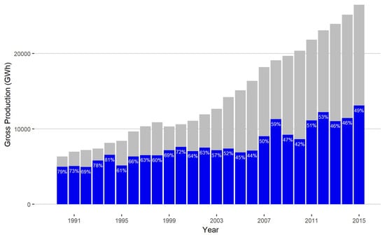
Figure 1.
Annual development of Ecuador’s electricity total generation. Blue bars represent the annual hydroelectric production with respect to the total generation.
Hence, Ecuador is currently implementing the National Master Plan for Electrification 2016–2025, which aims at covering more than 90% of the national electrical demand with hydroelectric sources [12]. The plan is already having an impact in Ecuador’s energy production capability [13]. Ecuador ranked third in the global list of countries that added more energy capacity in 2016, following China and Brazil [14]. By the end of that year, the installed hydroelectric capacity in Ecuador (4400 MW) represented 58% of the total capacity (7587 MW). Generation from hydroelectric systems in 2016 amounted to 57.9% (15,814.72 GWh) of the total production (27,313.86 GWh). In 2017, the installed capacity of the Ecuadorian electrical system increased to 8036 MW [15]. This year, Ecuador achieved energy sovereignty for the first time, i.e., the electricity production satisfied the national electricity demand and even 210 GWh were exported. Despite this fact, the maximum demand used only 47% of the produced electricity, i.e., 53% of the energy that can be generated is not used [16,17]. As a consequence, the management and planning of energy in Ecuador has room for improvement.
Energy production forecasts are of great importance to the operators of the electrical system (to optimize the processes) and the decisionmakers (to define better policies and manage risks). Besides, energy prices can be established considering the estimated future load demand. Therefore, it is crucial for an optimized energy system to accurately model the energy production and the energy demand to offer solutions at different levels of society [18].
The objective of this research work was to develop and apply forecasting models for predicting hydroelectric production in Ecuador from historical data. We focused on statistical time series analysis techniques, which have been successfully applied in the literature [19,20]. Since hydropower strongly depends on the meteorological conditions, rainfall data played a key role in our study. This data was easier to obtain than inflow, which was not available for the study. To the best of our knowledge, there is no similar study in the literature focused on the Ecuador case.
The contribution of this paper is twofold. First, it describes a methodology to model the production of hydroelectric plants through time series with the ARIMA univariate and ARIMAX bivariate approaches. Then, we present the application of this methodology to build and compare models for predicting production in Ecuador. Through the resulting model, the correlation between hydroelectric generation and precipitation is demonstrated and quantified. Furthermore, the paper shows that an ARIMAX model considering an exogenous variable (precipitation in one of the larger basins) can accurately predict monthly production values up to a year in advance. That implies that it is not necessary to use elaborated data to obtain a reliable prediction model. At the same time, this study improves the results obtained in a previous work which only considered ARIMA [21]. Accordingly, the methodology can be used to develop planning strategies in the energy sector in Ecuador. The applicability of the approach to other countries should be considered by future work.
2. Methods
2.1. Box-Jenkins and Box-Tiao Methods
Time series analysis comprises a wide collection of techniques for analyzing historical temporal data in order to extract meaningful features or characteristics of the data. A forecast model encodes a function that estimates the value of a prediction variable in the future from historical and other relevant data [22]. This prediction variable is usually also used in the input. In our case, the input and the prediction variable is energy production, and the additional variable is precipitation.
The accuracy of the model is measured as the difference between the predicted and the actual values. Learning a forecast model means fitting the model parameters to minimize this difference for a given dataset for which the input and the target values are known. It is expected that a forecast model will perform well with values outside the learning dataset. More details about time series analysis methods can be found in [23].
In the literature, we can find several methods to build forecast models from data. Among them, autoregressive models based on moving averages have proved effective in several problems [24]. In particular, there are applications of autoregressive models to predict renewable energy (wind, solar, hydro) production and demand [25,26,27,28,29,30,31,32,33].
Autoregressive models assume that observations are correlated through lagged linear relations and capture this correlation into the model. These models assume that the time series are stationary, i.e., the statistical properties, such as the mean, variance, and autocorrelation, are constant over time.
An autoregressive model of order p AR(p) is of the form:
where: Yt is the value of the prediction variable at time t (energy production, in this case), εt is a random variable with mean 0 and variance σ2w (white noise), and φ1 are the parameters of the models (constants). If we define the backshift operator B as BYt = Yt-1 (and recursively, BkYt = Yt-k), the equation can be rewritten as follows:
Yt = φ1Yt-1 + φ2Yt-2 + … + φpYt-p + εt
εt = (1 − φ1B − φ2B2 − … − φpBp) Yt = φp(B) Yt
The Box-Jenkins method identifies, adjusts, and checks a prediction model using an autoregressive integrated moving average (ARIMA) [34]. Box-Jenkins estimates the parameters of the model by applying the maximum likelihood. The model is formulated as follows:
where φp(B) is the autoregressive polynomial of order p, B is the backshift operator, Yt is the forecast variable which represents a white noise process with normal distribution N(0, σ2), d is the dth difference operator, φ0 is a numerical constant, θq(B) is the regular moving average (MA) polynomial of order q, and εt is the error of the model. These parameters (p, d, q) characterize the ARIMA model and must be identified a priori by analyzing the stationarity of the time series.
φp(B)(1 − B)dYt = φ0 + θq(B)εt
If the stationarity (S) is strong, ARIMA is extended to have two components: (1) One with regular structure ARIMA (p, d, q) that models the non-independence associated with the data, and (2) one with ARIMA structure (P, D, Q) that models the seasonality component. In this latter model, P is the autoregressive seasonal term, D is the seasonal term of difference, and Q corresponds to the seasonal term of moving average. A SARIMA model is formalized as follows:
where ΦP (Bs) is the autoregressive polynomial of order p with seasonality, ΘQ (Bs) is the regular moving average (MA) polynomial of order q with seasonality, D is the dth differential operator with seasonality, and B is the backshift operator with seasonality.
φp(B)ΦP (Bs)(1 − Bs)D(1 − B)d Yt = φ0 + θq(B) ΘQ (Bs)εt
The Box-Tiao method extends Box-Jenkins by incorporating the observations of the covariates, also called explanatory or exogenous variables X (ARIMAX). The ARIMAX model is described mathematically as follows:
φp(B)(1 − B)dYt = φ0 + Θ(B)Χt + θq(B)εt
The difference with respect to Equation (3) is the term Θ(B)Χt is the observed one, while Θ(B) is the polynomial operator of the exogenous variable Χt.
2.2. Time Series Analysis Process
In order to obtain the ARIMA and the ARIMAX models, we followed the methodology depicted in Figure 2. First, the time series were transformed to comply with the requirement that they must be stationary. Once the series were stationary, the parameters of the series were estimated through correlogram functions, which were associated with statistical tests. Afterward, different models were estimated to select the one that best fit the training data. The selected model was validated through residue analysis and hypothesis testing. Then, this model was tested with additional unseen data to calculate prediction accuracy. These steps are described in the following subsections.
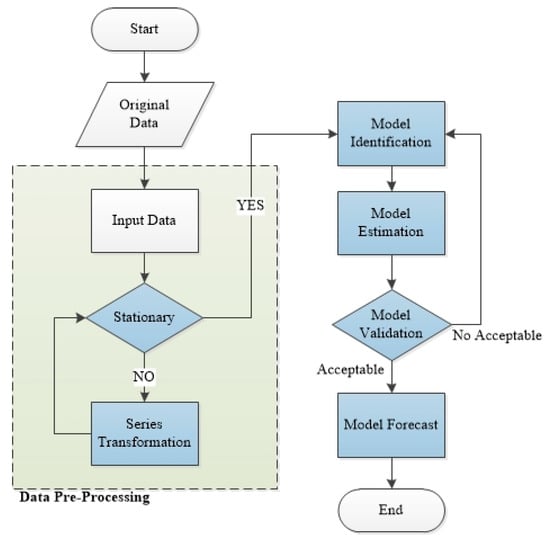
Figure 2.
Flowchart of the time series analysis methodology.
2.2.1. Series Transformation
The assumption of stationarity must be verified before the identification of a suitable model. A time series can be considered stationary if the mean and variance are constant and if there are no significant trends and seasonal variations. Usually, logarithm and derivative operations are applied to eliminate the variability and decrease the trend, respectively [23,35].
2.2.2. Stationary Evaluation
The single autocorrelation function (ACF) and partial autocorrelation function (PACF) are correlogram functions to determine the degree of correlation between two consecutive values of the series. ACF and PACF provide an estimation of the p and q values of the ARIMA models [36,37].
First, the single ACF and PACF functions of the transformed series were calculated and plotted. These functions are useful for diagnosing the p, d, q components of the ARIMA models.
The ACF of order k (k > 0) of a stationary process (Yt) measures the information that an observation of a period transmits directly to the observation k periods ahead, i.e., . It is presented with the following equation:
where γk is the self-covariance of order k, γo is the zero order self-covariance of a strictly stationary process, and .
The PACF measures the information that an observation of a period transmits directly to the observation k periods ahead, eliminating the information that both contain.
The PACF is denoted by φkk, for k = 1, 2, ... and represented with the following equations:
The first-order autocorrelation was formally tested with the Durbin-Watson statistic test [38], which measures the linear association between adjacent residuals. The null hypothesis for this case is that the series presents autocorrelation.
Second, the Augmented Dickey Fuller (ADF) test, also called the unit root test, was used to test the stationarity properties of the series [39,40].
2.2.3. Model Identification
Once the parameters (p, d, q) and (P, D, Q) were identified in previous stages, auto-regressive (AR), moving average (MA), seasonal auto-regressive (SAR), and eXogenous regressive (XREG) models were determined. The Equations (3)–(5) were used to identify the model that best fits each series.
2.2.4. Model Estimation
After the models were designed and implemented, the best model was selected considering penalized likelihood criteria, such as Akaike information criterion (AIC) and Bayesian information criterion (BIC) [41]. The AIC and BIC were used here to compare of models’ performance [23]. The AIC and BIC are described mathematically as follows:
where is the maximum likelihood estimate of variance, n is the number of dates, and, k is the number of parameters of the model.
The BIC strongly penalizes the number of involved parameters. High values of AIC mean that the observed data does not fit the models, while lower values indicate strong evidence that the observed data fit the models. Similarly, lower values of BIC indicate better fitting of the models.
2.2.5. Model Validation
In order to evaluate the prediction accuracy of the models of the Box-Jenkins and Box-Tiao, a residual analysis was performed. Before that, a first plot was done to analyze if whether there were atypical errors which indicated the need of an intervention.
In order for the ARIMA and ARIMAX models to be viable for the adjustments of the observed data, the error term εt in Equations (1)–(3) should behave as white noise, i.e., zero mean, a constant variance, and no correlation. In addition, the term εt must follow a normal distribution. To check these assumptions, statistical tests should be applied to the residuals, as in [23,26].
The most widely used model is the Box-Ljung test [36], with the null hypothesis being that the series is uncorrelated. Accordingly, a Box-Ljung test was applied to the (squared) residuals to verify that the variance is constant. Afterward, the Jarque-Bera test [42] was applied to verify that the residuals were normal. In our experiments, these tests were applied to the significance level of α = 0.05.
2.2.6. Model Forecast
Once the ARIMA and ARIMAX models have been validated, future time series values can be forecasted. In our case, energy production was forecasted for a 12-month horizon corresponding to the year 2015, with a typical 95% confidence interval (CI) [22].
2.3. Measures of Accuracy
In order to evaluate the quality of forecasted data of the proposed models, statistical analysis of errors was used. Three typical standards were selected in this research work: Mean absolute error (MAE), mean absolute percentage error (MAPE), and mean absolute scaled error (MASE).
The MAE represents the average error value between the observed and the adjusted series. The MAE is described mathematically as follows:
where vadj represents the individual value of the forecasted time series, vobs corresponds to the individual value of the observed time series, and n is the order of the series. In this study, the MAE is measured in gigawatt hours (GWh) since the predicted variable is hydroelectric production.
The mean absolute percentage error (MAPE) is another statistical parameter considered in this study. The advantage of using this parameter is that it uses percentages (%) to show the data, which allows an easy and quick evaluation of the predicted model [30]. The MAPE is described mathematically as follows:
Finally, the mean absolute scaled error (MASE) was considered in the analysis. This type of error is independent of the data. Lower values of scaled error (qt) result in better forecasts [43,44]. The MASE is described mathematically as follows:
where et represents the error between adjusted and observed values.
3. Data
Data for the current study, corresponding to the 2000–2015 period, have been obtained from official and governmental institutions of Ecuador, namely the Electricity Regulation and Control Agency (ARCONEL) [11] and the National Institute of Meteorology and Hydrology (INAMHI) [45]. The modeling analysis considers the period from 2000 to 2014, and 2015 data were used to validate the predictivity of the model.
In this section, we present information about the Ecuadorian hydroelectric system, the country’s hydrographic basins, the regions and the dataset used in this work, and the time series used to build the models.
3.1. Ecuadorian Hydroelectric System
The hydroelectric system in Ecuador is concentrated in a relatively small group of stations. In 2016, the 13 largest power stations provided 89.57% of the total hydroelectric generation. Table 1 shows the contributions of hydroelectric generation grouped by management company and geographical region of watersheds in detail.

Table 1.
Electric production of the country’s 13 largest hydropower stations during 2016.
Coca Codo Sinclair is the largest hydroelectric power plant in the country. Over the next years, this plant is expected to have 1500 MW of power and satisfy 35% of the country demand. The socioeconomic and environmental impacts of this project have been largely studied [46,47,48], but its management and planning has received less attention.
3.2. Rainfall and Watersheds in Ecuador
The estimated water potential, at the level of river basins and sub-basins, is about 15,000 m3/s distributed on the Ecuadorian continental surface. Its potential is geographically distributed in two regions: Amazon (east) and Pacific (west), with a flow capacity of 71% and 29%, respectively, according to the National Water Resources Council (CNRH) [55]. Twenty-four watersheds are inside the Pacific area and seven watersheds are inside the Amazon area. The area of the latter is 131,726 km2, which corresponds to 51% of the country’s hydrographic system.
In Ecuador, the following values of the hydroelectric potential have been identified: (i) Medium theoretical hydroelectric potential, with an estimated average monthly flow of 91,000 MW; (ii) technically feasible potential: 31,000 MW (in 11 watersheds); and (iii) economically feasible potential: 22,000 MW (in 11 watersheds). Currently, Ecuador has used 24.55% of the economically feasible potential, i.e., 5401 MW [12].
3.3. Regions of Study and Dataset
Evidently, water is the main resource to produce power hydroelectric. Therefore, water inflow is a good predictor of hydroelectric performance [20,21]. In this study, we used precipitation data as a proxy for hydropower stations water inflow. Precipitation data are relevant because the regions of the study have a considerable rainfall variability, since they are located within a region with warm-humid climate [56]. Besides, precipitation data are typically used in weather derivatives [57], which are financial instruments that cover the effects of adverse or unexpected weather conditions. Consequently, they are a usual input in the decision-making process.
Note that the precipitation value is not an estimation of the inflow, but a potential predictor. In the literature, there are other works using streamflow data collected from sensors installed in the reservoirs [58,59]. Such approaches provide more accurate water inflow estimations but are also more costly to implement at a larger scale. At the time of this study, these data were not available in Ecuador. An alternative to consider in the future is to use stochastic models to generate this data [60,61].
We considered precipitation data from the three main Amazon watersheds, namely:
- Napo, with an area of 59,505 km2 fed by 15 rivers.
- Pastaza, with an area of 23,190 km2 fed by 11 rivers.
- Santiago with an area 24,920 km2 fed by four rivers.
The three basins add up an area of 107,615 km2, which represent about 82% of the Amazon hydrological system and 42% of the country’s total. They contain the 12 largest hydroelectric stations, generating about 82% of the hydropower production, as shown in Table 1.
Following the aim of the paper, we wanted to improve production forecasts by considering a minimum but significant amount of additional data, i.e., precipitation data. Precipitation data corresponding to the period 2000–2015 were obtained from pluviometric stations (PS) located inside the basins and managed by the INAMHI: Napo (13 PS), Pastaza (27 PS) and Santiago (28 PS). Figure 3 shows the geographical location of each PS inside their corresponding watersheds.
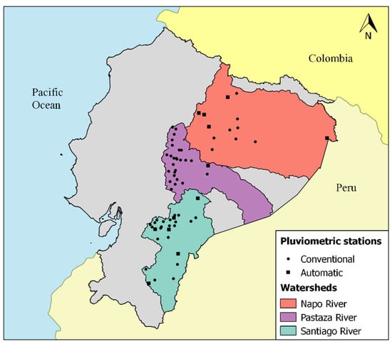
Figure 3.
Geographical location of conventional and automatic pluviometric stations.
The source data included a single data point per station and month, representing the total rainfall measured by the station in the month. To obtain a single value per basin and month, we averaged these values for each basin. In this way, we have a single value for each basin representing a rough approximation of the expected monthly rainfall at any randomly selected point inside the basin. Furthermore, we assumed that basins are independent and thus aggregated the three monthly values to obtain the overall rainfall that can be potentially used to produce energy. Certainly, this entails a considerable simplification of the problem, and other aggregation methods could be considered.
Figure 4 shows the water shortage that normally occurs on the Amazon region from October to March [62]. The aggregated expected rainfall in the Napo, Pastaza, and Santiago basins is represented by the blue bar chart. The average of the total precipitation during these two years was 466.5 mm (black line). Precipitation in the months of October to March, in general, is below the average of the total precipitation since these months correspond to the Ecuadorian dry season. This drought influences the hydroelectric systems, which is evident in the curve of hydroelectric production.
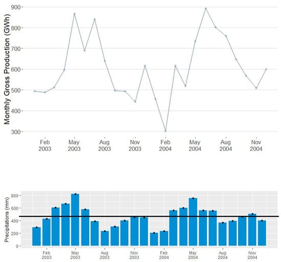
Figure 4.
Monthly hydroelectric production and total precipitation of the three considered watersheds during 2003–2004.
3.4. Time Series
The following five series have been considered during the period 2000–2014:
- Monthly gross production (MGP) of hydroelectric systems [GWh];
- Average monthly precipitation (AMP) in Napo watershed [mm];
- AMP in Pastaza watershed [mm];
- AMP in Santiago watershed [mm];
- Total average monthly precipitation (TAMP) in the three considered watersheds [mm]
To know the behavior and better fit in the analysis of the modeling, an analysis of each one of the five series was performed. Correlations between pairs of series were also studied, in particular, MGP-AMPNapo, MGP-AMPPastaza, MGP-AMPSantiago, and MGP-TAMP.
4. Experiments and Discussion
4.1. Exploratory Data Analysis and Series Transformation
Figure 5 shows the AMP of the Napo, Pastaza, and Santiago watersheds and MGP series during the period 2000–2014. All series show a direct correlation, i.e., as precipitation increases or decreases in watersheds, the production of hydropower increases or decreases. Also, the AMP of the watersheds is correlated with the MGP series. Moreover, the MGP series presents variability and trend over time, in contrast to AMP series that show variability but no trend through the time.
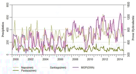
Figure 5.
Time series of precipitation [mm] at river basins and hydroelectric production [GWh] in Ecuador, 2000–2014.
The three series of precipitation data show stationarity and seasonality. The hydroelectric production series that does not show stationarity but seasonality. As part of the study, the hydroelectric production series was transformed to make it stationary.
Figure 6 depicts the cross-correlation function (CCF) between two series at lag k, estimated as follows: If the simple cross-correlation is larger than the standard deviation error, CCF is considered significantly different from zero. When the joint series show correlation, it is necessary to separate the linear association to make them stationary. In the separation step, the residuals of the model are transformed into white noise in a process known as (pre-)whitening. In ARIMA models, through the correlogram functions ACF-PACF, the possible order values (p, d, q) are diagnosed to eliminate the trend and variability. In contrast, the dynamic relationship between two series is analyzed through the cross-correlation function adjusted to pre-whitened residuals [34], to estimate the best ARIMAX model.
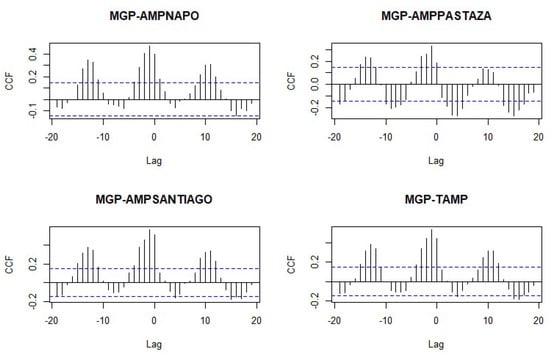
Figure 6.
Cross-correlation function between precipitation and power hydroelectric.
4.2. Hydroelectric Energy Generation Modeled with ARIMA
Now we can proceed to the model identification step described in Figure 2. First, we focused on the ARIMA model.
Figure 7a presents the autocorrelation functions ACF and PACF used to evaluate stationary after pre-whitening. Both functions decay exponentially in a delay or lag of 5, which is significant with seasonal frequencies suggested by the SARIMA model. Figure 7b shows the same functions applied to the series of differences. The value of the Durbin-Watson statistic parameter obtained is 1.98, so the series presents evidence of weak positive autocorrelation.
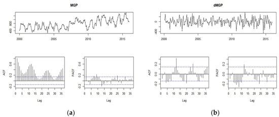
Figure 7.
ACF and PACF autocorrelation functions (see Section 2.2.2). (a) Correlogram functions of the monthly gross production (MGP) series; (b) correlogram functions of the differenced MGP series.
For the analysis of the stationarity of the MGP series, we obtained the ADF statistics, whose value was t-ADF = −8.77 with a p-value of 0.01. There is significant evidence that the series is stationary and has no unit roots, with a maximum delay of 13 months. To determine the variants, the regression test was used to derive the ADF test which resulted to be significant with a value t = −15.06 at α = 0.05 of significance level. This means that the series shows a random walk with mean zero.
Once we know that the series is stationary, we can step into the model identification stage. Table 2 shows a summary of the results obtained by applying the Box-Jenkins method to the MGP series. Figure 8 depicts comparison between actual and predicted values. The model minimizing AIC and BIC was ARIMA (1,1,1) × (0,0,1)12 with random walk. The model was confirmed to satisfy the assumptions of the SARIMA model. The validation results with the 2015 data were within the designated confidence interval.
Table 2.
Box-Jenkins method applied in MGP series.
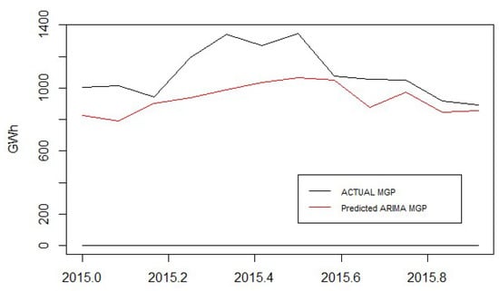
Figure 8.
Comparison between actual and predicted values with the ARIMA model.
4.3. Hydroelectric Energy Generation Modelled with ARIMAX
Regarding the ARIMAX model, the amount of precipitation at each watershed was considered as the exogenous variable. The steps described in Section 2 produced the results presented below.
Figure 9 shows the residual diagnosis of each pair of series. The following characteristics were found: (i) Each series did not present outliers; (ii) each pair of series was uncorrelated; (iii) ACF lags were not significant; and iv) the p-value of the Ljung-Box test was greater than 0.05, which indicates that the squared residuals were uncorrelated over time, i.e., the standardized residuals were independent.
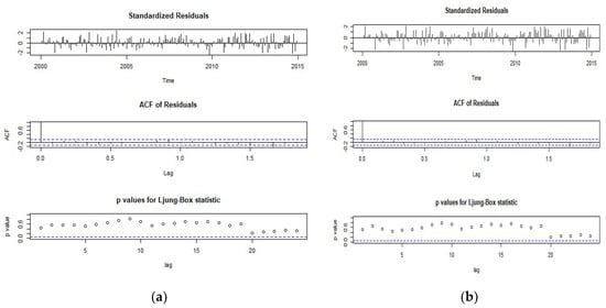
Figure 9.
Residual diagnosis of each pair of series. (a) Correlogram MGP-AMPPASTAZA average monthly precipitation AMPPASTAZA; (b) series MGP-AMPNAPO; (c) Correlogram MGP-AMPSANTIAGO; (d) series MGP-TAMP.
Table 3 shows the coefficients of the best ARIMAX models for hydroelectric production with the exogenous variable. The model with the lowest AIC and BIC is the pair of MGP-AMPSANTIAGO series. Figure 10 shows the forecasts of each ARIMAX model for the year 2015.
Table 3.
Box-Tiao method applied in MGP series with exogenous variable.
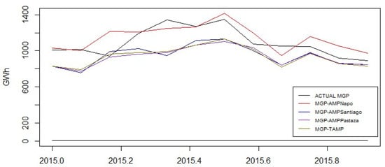
Figure 10.
Comparison between actual and predicted values 2015 with ARIMAX Models.
4.4. Comparison and Discussion
Table 4 shows the MAE, MAPE, and MASE of the forecasts of each model for the year 2015. It can be seen that the best results (lower error) were obtained by the ARIMAX model of MGP-AMPNAPO. This is corroborated in Figure 10, which indicates that MGP-AMPNAPO was better.
Table 4.
Forecast errors of each model.
Figure 11 visually shows the forecast of hydroelectric production in Ecuador for 2015, considering ARIMA and ARIMAX models. A better forecast was obtained with the ARIMAX models of MGP-AMPNAPO.
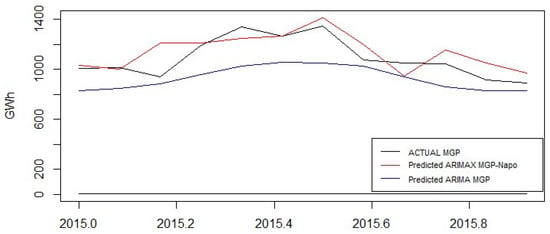
Figure 11.
Predicted values comparison of ARIMA and ARIMAX models.
Although the ARIMAX model of MGP-AMPSATIAGO has the best estimation model considering the AIC and BIC values, ARIMAX model MGP-AMPNAPO has the lower forecast error values. Hence, ARIMAX model MGP-AMPNAPO was selected.
Figure 11 depicts that ARIMAX MGP-AMPNAPO (1,1,1)(1,0,0)12 model presented a better predictivity of gross monthly hydroelectric energy production in Ecuador. This model estimated that the occurrence of the production is for the parameter p = 1 and a suitable moving average of q = 1 for the regular component. At the same time, for seasonal component, P = 1 and the strong seasonality established as S = 12. The exogenous variable are precipitation values at Napo watershed. The value of MAE is 70.81 GWh, MAPE is 10.17%, and MASE is 0.57.
5. Conclusions
This work shows that the ARIMAX models with an exogenous variable have better performance than the univariate ARIMA models for predicting hydroelectric energy production in Ecuador. Our analysis of the production and the precipitation of the Napo, Pastaza, and Santiago basins (alone and aggregated) yielded that the ARIMAX MGP-AMPNAPO (1,1,1)(1,0,0)12 model adequately adjusts the data of the hydroelectric energy production in Ecuador series.
This research helps to describe and predict hydropower generation, particularly in Ecuador. Results obtained with the proposed model can be useful for the organizing and planning of the electric sector, which are important for the energy policymaker sector. The methodology can be also extended to use in other cases.
Further studies to improve the accuracy of the predictions can be performed including bioinspired techniques and optimization algorithms. Besides, we plan to study the impact of incorporating additional data sources to the model, e.g., synthetic streamflow data, as mentioned in Section 3.3, or other weather parameters, like wind, rain, etc. The applicability of the approach to other countries remains as future work.
Author Contributions
J.B.-M.: Conceptualization, Methodology, Data curation, Writing—Original Draft, Writing—Review & Editing. M.M.-L.: Methodology, Software, Validation, Formal Analysis. M.E.-A.: Formal Analysis, Writing—Review & Editing. J.G.-R.: Writing—Review & Editing, Visualization, Supervision. W.F.: Writing—Review & Editing, Supervision.
Funding
This work has been funded by the Universidad de Guayaquil through the grant number FCI-015-2019. This work has been also supported by ESPOL, grant number FIMCP-CERA-05-2017.
Acknowledgments
The authors kindly acknowledge the support from University of Guayaquil. Computational and physical resources were provided by ESPOL. Juan Gómez-Romero is partially supported by the University of Granada (P9-2014-ING) and the Spanish Ministries of Science, Innovation and Universities (TIN2017-91223- EXP) and Economy and Competitiveness (TIN2015-64776-C3-1-R).
Conflicts of Interest
The authors declare no conflict of interest.
References
- International Energy Agency (IEA). Key World Energy Statistics 2018. Available online: https://webstore.iea.org/key-world-energy-statistics-2018 (accessed on 26 February 2019).
- International Energy Agency (IEA). Electricity Information: Overview 2018. Available online: https://webstore.iea.org/electricity-information-2018-overview (accessed on 26 February 2019).
- Sher, F.; Pans, M.A.; Afilaka, D.T.; Sun, C.; Liu, H. Experimental investigation of woody and non-woody biomass combustion in a bubbling fluidised bed combustor focusing on gaseous emissions and temperature profiles. Energy 2017, 141, 2069–2080. [Google Scholar] [CrossRef]
- Sher, F.; Pans, M.A.; Sun, C.; Snape, C.; Liu, H. Oxy-fuel combustion study of biomass fuels in a 20 kWth fluidized bed combustor. Fuel 2018, 215, 778–786. [Google Scholar] [CrossRef]
- Zhang, Y.; Fang, Y.; Jin, B.; Zhang, Y.; Zhou, C.; Sher, F. Effect of Slot Wall Jet on Combustion Process in a 660 MW Opposed Wall Fired Pulverized Coal Boiler. Int. J. Chem. React. Eng. 2019, 17, 1–13. [Google Scholar] [CrossRef]
- Cevallos-Sierra, J.; Ramos-Martin, J. Spatial assessment of the potential of renewable energy: The case of Ecuador. Renew. Sustain. Energy Rev. 2018, 81, 1154–1165. [Google Scholar] [CrossRef]
- Barzola-Monteses, J.; Espinoza-Andaluz, M. Performance Analysis of Hybrid Solar/H2/Battery Renewable Energy System for Residential Electrification. In Proceedings of the 10th International Conference Application Energy, Hong Kong, China, 22–25 August 2018; Elsevier: Hong Kong, China, 2018. [Google Scholar]
- UASB-DIGITAL. ¿Es sustentable la política energética en el Ecuador? Available online: http://hdl.handle.net/10644/3036 (accessed on 11 March 2019).
- Buñay, F.; Pérez, F. Comparación de Costos de Producción de Energía Eléctrica Para Diferentes Tecnologías en el Ecuador. Bachelor’s Thesis, Universidad de Cuenca, Cuenca, Spain, 2012. [Google Scholar]
- Carvajal, P.E.; Li, F.G.N.; Soria, R.; Cronin, J.; Anandarajah, G.; Mulugetta, Y. Large hydropower, decarbonisation and climate change uncertainty: Modelling power sector pathways for Ecuador. Energy Strateg. Rev. 2019, 23, 86–99. [Google Scholar] [CrossRef]
- Agencia de Regulación y Control de Electricidad (ARCONEL). Available online: https://www.regulacionelectrica.gob.ec/ (accessed on 3 January 2019).
- Ministerio de Electricidad y Energía Renovable (MEER). Plan Maestro de Electricidad 2016–2025; ARCONEL: Quito, Ecuador, 2016; pp. 1–440.
- Agencia de Regulación y Control de Electricidad (ARCONEL). Estadística Anual y Multianual del Sector Eléctrico Ecuatoriano (2016); ARCONEL: Quito, Ecuador, 2016.
- International Hydropower Association (IHA). Hydropower Status Report; IHA: London, UK, 2017. [Google Scholar]
- Ministerio de Electricidad y Energía Renovable (MEER). Rendición de cuentas MEER 2017; MEER: Quito, Ecuador, 2017; pp. 1–39.
- Ordoñez, L. Centro de Investigación y Capacitación Eléctrica. Available online: https://cicecuador.org/ (accessed on 2 January 2019).
- Operador Nacional de Electricidad (CENACE). Available online: http://www.cenace.org.ec/docs/InformacionOperativa.htm (accessed on 2 January 2019).
- Elamin, N.; Fukushige, M. Modeling and forecasting hourly electricity demand by SARIMAX with interactions. Energy 2018, 165, 257–268. [Google Scholar] [CrossRef]
- Koivisto, M.; Das, K.; Guo, F.; Sørensen, P.; Nuño, E.; Cutululis, N.; Maule, P. Using time series simulation tools for assessing the effects of variable renewable energy generation on power and energy systems. WIREs Energy Environ. 2019, 8, 1–15. [Google Scholar] [CrossRef]
- Dehghani, M.; Riahi-Madvar, H.; Hooshyaripor, F.; Mosavi, A.; Shamshirband, S.; Zavadskas, E.K.; Chau, K. Prediction of hydropower generation using grey Wolf optimization adaptive neuro-fuzzy inference system. Energies 2019, 12, 289. [Google Scholar] [CrossRef]
- Mite-León, M.; Barzola-Monteses, J. Statistical Model for the Forecast of Hydropower Production in Ecuador. Int. J. Renew. Energy Res. 2018, 10, 1130–1137. [Google Scholar]
- Hyndman, R.J.; Athanasopoulos, G. Forecasting: Principles and Practice, 2nd ed.; OTexts: Melbourne, Australia, 2018. [Google Scholar]
- Shumway, R.H.; Stoffer, D.S. Time Series Analysis and Its Applications with R Example, 4th ed.; Springer: Pittsburgh, PA, USA, 2017. [Google Scholar]
- Maçaira, P.M.; Marcio, A.; Thomé, T.; Luiz, F.; Oliveira, C. Time series analysis with explanatory variables: A systematic literature review. Environ. Model. Softw. 2018, 107, 199–209. [Google Scholar] [CrossRef]
- Raza, M.Q.; Nadarajah, M.; Ekanayake, C. On recent advances in PV output power forecast. Sol. Energy 2016, 136, 125–144. [Google Scholar] [CrossRef]
- Camelo, N.; Sérgio, P.; Bosco, J.; Leal, V.; Cesar, P.; Carvalho, M.D. A hybrid model based on time series models and neural network for forecasting wind speed in the Brazilian northeast region. Sustain. Energy Technol. Assess. 2018, 28, 65–72. [Google Scholar]
- Soman, S.S.; Zareipour, H.; Malik, O.; Mandal, P. A review of wind power and wind speed forecasting methods with different time horizons. In Proceedings of the North American Power Symposium 2010, Arlington, TX, USA, 26–28 September 2010; pp. 1–8. [Google Scholar]
- Kim, D.; Hur, J. Short-term probabilistic forecasting of wind energy resources using the enhanced ensemble method. Energy 2018, 157, 211–226. [Google Scholar] [CrossRef]
- Lee, Y.; Hur, J. A simultaneous approach implementing wind-powered electric vehicle charging stations for charging demand dispersion. Renew. Energy 2019, 144, 172–179. [Google Scholar] [CrossRef]
- Camelo, H.; Lucio, P.S.; Leal Junior, J.B.V.; Marques de Carvalho, P.C.; Glehn dos Santos, D. Innovative hybrid models for forecasting time series applied in wind generation based on the combination of time series models with artificial neural networks. Energy 2018, 151, 347–357. [Google Scholar] [CrossRef]
- Inman, R.H.; Pedro, H.T.C.; Coimbra, C.F.M. Solar forecasting methods for renewable energy integration. Prog. Energy Combust. Sci. 2013, 39, 535–576. [Google Scholar] [CrossRef]
- Pektas, A.O.; Cigizoglu, H.K. ANN hybrid model versus ARIMA and ARIMAX models of runoff coefficient. J. Hydrol. 2013, 500, 21–36. [Google Scholar] [CrossRef]
- Suganthi, L.; Samuel, A.A. Energy models for demand forecasting—A review. Renew. Sustain. Energy Rev. 2012, 16, 1223–1240. [Google Scholar] [CrossRef]
- Box, G.E.P.; Jenkings, G.; Reinsel, G. Time Series Analysis; Prentice Hall: New Jersey, NJ, USA, 1994. [Google Scholar]
- Cryer, J.D.; Chan, K.S. Time Series Analysis with Applications in R, 2th ed.; Springer: Iowa City, IA, USA, 2008. [Google Scholar]
- Box, G.E.P.; Pierce, D.A. Distribution of Residual Autocorrelations in Autoregressive Integrated Moving Average Time Series Models. J. Am. Stat. Assoc. 1970, 65, 1509–1526. [Google Scholar] [CrossRef]
- Box, G.E.P.; Jenkins, G.M. Time Series Analysis: Forecasting and Control, Revised ed.; Holden-Day: Oakland, CA, USA, 1976. [Google Scholar]
- Kramer, W. Durbin-Watson Test. In International Encyclopedia of Statistical Science; Lovric, M., Ed.; Springer: Kragujevac, Serbia, 2011. [Google Scholar]
- Dickey, D.A.; Fuller, W.A. Likelihood Ratio Statistics for Autoregressive Time Series with a Unit Root. Econometrica 1981, 49, 1057–1072. [Google Scholar] [CrossRef]
- Said, S.E.; Dickey, D.A. Testing for unit roots in autoregressive-moving average models of unknown order. Biometrika 1984, 71, 599–607. [Google Scholar] [CrossRef]
- Schwarz, G. Estimating the dimension of a model. Ann. Stat. 1978, 6, 461–464. [Google Scholar] [CrossRef]
- Pfaff, B. VAR, SVAR and SVEC Models: Implementation Within R Package Vars. J. Stat. Softw. 2008, 27, 1–32. [Google Scholar] [CrossRef]
- Hyndman, R.J.; Koehler, A.B. Another look at measures of forecast accuracy. Int. J. Forecast 2006, 22, 679–688. [Google Scholar] [CrossRef]
- Franses, P.H. A note on the Mean Absolute Scaled Error. Int. J. Forecast 2016, 32, 20–22. [Google Scholar] [CrossRef]
- Instituto Nacional de Meteorología e Hidrología (INAMHI). Available online: http://www.serviciometeorologico.gob.ec/ (accessed on 3 January 2019).
- Rodríguez Carreño, M.G. Impacto del Proyecto Hidroeléctrico Coca Codo Sinclair en la Matriz Energética Como Generador de Oportunidades del Ecuador en el Mundo. Bachelor’s Thesis, Universidad del Azuay, Cuenca, Spain, 2015. [Google Scholar]
- Chen, Y. Impacto Socio-Económico del Proyecto Hidroeléctrico Coca Codo Sinclair, Construido por la Empresa China Sinohydro, Para la Economía Ecuatoriana. Bachelor’s Thesis, Pontificia Universidad Católica del Ecuador, Quito, Ecuador, 2015. [Google Scholar]
- López, V. El proyecto hidroeléctrico Coca Codo Sinclair y la gobernanza energética en la Amazonía ecuatoriana. Let. Verdes 2011, 8, 1–3. [Google Scholar] [CrossRef][Green Version]
- Corporación Eléctrica del Ecuador (CELEC). Available online: https://www.celec.gob.ec/ (accessed on 5 March 2019).
- CELEC—Hidropaute 2019. Available online: https://www.celec.gob.ec/hidropaute/ (accessed on 5 March 2019).
- CELEC—Coca Codo Sinclair 2019. Available online: https://www.celec.gob.ec/cocacodosinclair/ (accessed on 5 March 2019).
- CELEC—Hidroagoyán 2019. Available online: https://www.celec.gob.ec/hidroagoyan/ (accessed on 5 March 2019).
- CELEC—Hidronación 2019. Available online: https://www.celec.gob.ec/hidronacion/ (accessed on 5 March 2019).
- Electro Generadora del Austro (ELECAUSTRO). Available online: http://www.elecaustro.com.ec/ (accessed on 5 March 2019).
- Consejo Nacional de Recursos Hídricos (CNRH). División Hidrográfica del Ecuador; Ministerio del Ambiente: Quito, Ecuador, 2002.
- Laraque, A.; Loup Guyot, J.; Pombosa, R. Hidroclimatología del Oriente e Hidrosedimentología de la Cuenca del Napo. La Cuenca Oriente Geol. y Petróleo; Institut Français d’études Andines: Quito, Ecuador, 2004; pp. 131–351. [Google Scholar]
- Hernández, J.; Carvajal-Serna, F. Cobertura al riesgo ante la variabilidad hidrológica en una central hidráulica a filo de agua usando derivados climáticos. Lect. Econ. 2017, 87, 191–222. [Google Scholar] [CrossRef]
- Aronica, G.T.; Bonaccorso, B. Climate change effects on hydropower potential in the Alcantara River basin in Sicily (Italy). Earth Interact 2013, 17, 1–22. [Google Scholar] [CrossRef]
- Can, I.; Tosunoǧlu, F. The estimation of the firm hydroelectric potential of the Çoruh Basin, Turkey. Energy Sources Part A Recover Util. Environ. Eff. 2012, 34, 1609–1618. [Google Scholar] [CrossRef]
- Dashora, I.; Singal, S.K.; Srivastav, D.K. Streamflow prediction for estimation of hydropower potential. Water Energy Int. 2015, 57, 54–60. [Google Scholar]
- Zhao, T.; Zhao, J. Forecast-skill-based simulation of streamflow forecasts. Adv. Water Resour. 2014, 71, 55–64. [Google Scholar] [CrossRef]
- Cevallos Escobar, J.G.; Macas Díaz, D.F. Análisis de la Complementariedad Hidrológica de las Vertientes del Amazonas y del Pacífico en el Ecuador Considerando las Nuevas Centrales Hidroeléctricas Proyectadas Hasta el Año 2016. Ph.D. Thesis, Escuela Politécnica Nacional, Quito, Ecuador, 2012. [Google Scholar]
© 2019 by the authors. Licensee MDPI, Basel, Switzerland. This article is an open access article distributed under the terms and conditions of the Creative Commons Attribution (CC BY) license (http://creativecommons.org/licenses/by/4.0/).