Optimization of a Bikeway Network with Selective Nodes

Abstract

Setting up a bikeway network has been recognized as one of the most effective measures to motivate cycling. In fact, a highly connected, exclusive bikeway network that covers all demand sources can be an attractive and time-saving measure, but it requires very high setup costs. The planner often needs to have a trade-off between demand coverage and travel time under a given construction cost. This paper introduces a novel bikeway design problem which determines an optimal bikeway network that covers all potential cycling demand sources with minimal total travel time and under budget constraints. In the context of designing a bike sharing system, the resultant node set of the bikeway network can be interpreted as the locations of the shared bike stations which can cover all cycling demands. A two-stage solution method, by combining the genetic algorithm and a novel elimination heuristic, is proposed to solve the problem by firstly determining the subset of nodes (selected nodes) that can cover all the demand sources and then designing the bikeway network that connects all selected nodes within a given budget. Numerical studies illustrate the advantages of elimination heuristics in solving the proposed problem and the effect of the budget towards the solution fitness with or without a solution. Case studies of two proposed new towns in Hong Kong are provided to illustrate the applicability and effectiveness of the method in bikeway design. This optimization model can be applied to bike-sharing system design problems which aims to cover all demand sources by providing bike stations that are also well connected with exclusive bikeways subject to budget constraints.

1. Introduction

Cycling has been receiving attention in the past decade due to its associated benefits, including improving public health, reducing greenhouse gas emissions, alleviating traffic congestion, and increasing the catchment area of public transportation [1]. It is competitive with cars for short trips in urban regions, as it has a lower total travel cost and sometimes a shorter travel time as well [2]. These benefits have motivated a worldwide development of bicycle networks and public bike-sharing systems (PBSs) [3]. At present, there are more than 1,500 PBSs with more than 17 million bicycles in operation [4].

The provision of a connected bikeway network has been proven to be one of the main measures to motivate cycling because it greatly improves cyclists’ safety (e.g., references [1,5]). Buehler and Pucher [6] revealed three critical elements that a bikeway network can use to increase cycling levels, including (1) separation with the roadway traffic, (2) high continuity and connectivity, and (3) high bikeway density. These elements can also be internalized in other complex measures such as a bicycle level of service (BLOS), bicycle compatibility index, or level of traffic stress. In other words, a bikeway network that can motivate cycling should be a dense network of exclusive and continuous bikeways, in which the cyclists can ride safely and encounter fewer detours. It is noted that these elements are also implicitly covered in the existing bikeway network design models. The bikeways (and the intersections) are required to meet a predefined level of service, and the trip lengths for the origin-destination pairs should be minimized or below a predefined upper bound ([2,7]). Though the setup of exclusive bikeways offers a safer cycling environment, its adverse impacts on the existing traffic (e.g., reducing the roadway capacity or on-street parking spaces) should be addressed in order to achieve a balance between the performance of the bikeway and the roadway networks. This introduces bikeway network design problems involving a co-existing roadway network (e.g., references [8,9]).

In addition to these elements, the bikeway network design needs to consider the trade-off between the travel time between every origin-destination (O-D) pair and the bikeway construction costs. By increasing the bikeway density, the travel times between the O-D pairs can be reduced, and more cycling activities can thus be motivated ([2,10]). However, higher bikeway density incurs a higher bikeway setup cost. Since the setup costs for a bikeway network are often limited, there is a question on how a bikeway design that minimizes total travel times for all cyclists can be achieved under the budget constraint. However, previous bikeway design studies have not addressed this question and only focus on either cost minimization or travel time minimization (e.g., references [2,7,9]). On the other hand, a bikeway network needs to handle its service coverage. A common approach is to assume an aggregated demand at each potential bike station, while the objective of the bikeway network design is to connect all potential stations with minimal costs in order to cover all demands. However, this approach neglects the fact that the demand points (e.g., transport interchanges, tourist spots, and schools) are not located exactly at but instead close to all potential nodes: as long as there is one station proximate to a demand point, the bikeway network can cover that demand point. In other words, it is sufficient to cover all demands by selecting a set of nodes among all potential nodes (this set of nodes can be named as a selected node set), and the bikeway layout that connects these selected nodes must have a lower construction cost than that connects all potential nodes. This concept of demand coverage is modeled in bike station location design (e.g., reference [11]) but never in bikeway network design, which is used to determine the selected node set and connect these nodes by using bikeways. This study, therefore, proposes a new bikeway design problem that minimizes the total system travel time between the selected nodes under both the budget and demand coverage constraints.

As the above novel problem involves two types of discrete decisions (i.e., locations of the selected nodes and built bikeways), this study prefers to develop a two-stage heuristic to solve the proposed problem. The first stage node selection is solved by the classic Genetic Algorithm, which has proved to be powerful in solving many combinatorial problems (e.g., reference [12]). Meanwhile, this stage can also be solved by other meta-heuristics (e.g., a tabu search and large neighborhood search). Nevertheless, no existing heuristic is applicable to solve the second-stage bikeway construction. As a congestion-free transport mode, the travel time of the bikeway is always assumed to be flow-independent and constant (e.g., reference [7]), and therefore the optimal route for all cyclists of each O-D pair is equivalent to the lowest cost route. Nevertheless, this problem is not equivalent to the shortest path problem because of the budget constraint. The overall bikeway construction cost is limited and sometimes needs to be minimized, which is similar to the minimum spanning tree problem or Steiner tree problem.

Table 1. Comparisons of existing shortest path and minimum spanning tree problems.

Problem Type		Design Objective	Examples of Existing Heuristics
Source	Sink
1	1	Minimize travel time between a node pair	Dijkstra’s algorithm [13]
1	All	Minimize total edge cost that connects a single source to all other nodes	Prim’s algorithm [14] Kruskal’s algorithm [15]
All	All	Minimize total travel time between all node pairs	Floyd-Warshall algorithm [16,17]
1	Some	Minimize total edge cost from a single source to a subset of nodes	Kou, Markowsky, and Berman algorithm [18]
Some	Some	Minimize total travel time between all node pairs within a subset of nodes	This study

compares the common shortest path problems and minimum spanning tree problems with respect to the number of origins and destinations considered in these problems and lists out their design objectives, and the common heuristics used to solve these problems (i.e., references [13,14,15,16,17,18]). Regarding the problem type, “1”, “all”, and “some” represent the number of nodes chosen to be the origins/ destinations, in which “some” indicates that a subset of nodes among all nodes are selected to be the origins/ destinations (which cannot be “one” or “all”). It is noted that unselected nodes can be included in the “selective” case if they can reduce the total cost and maintain the connectivity of the selected nodes. The design objectives can be classified into two classes, cost (weight) minimization, and travel time minimization. The former aims to determine a network that connects the nodes with minimal weight, and the latter aims for a set of minimal cost routes between the origin(s) and the destination(s). In other words, the former guarantees a minimal overall construction cost while the latter provides minimal travel costs between the O-D pairs, but none of them can provide an intermediate solution, which is a network with minimal total travel time under a given budget, especially in the case with a selected set of nodes. In addition, the studied problem should be distinguished from the Generalized Minimum Spanning Tree (G-MST) problem [19] which aims to connect part of the nodes in the network with minimum construction cost. In G-MST, each node has been firstly allocated to a group, and the resultant network requires that all groups should be connected, which implies that at least one node in each group is required to be connected. However, this study does not have any predefined group as not all nodes are selected, so the requirement that at least one element in each group cannot be held. As the studied problem differs from the above-discussed problems significantly, the heuristics used in those problems cannot be applied directly and thus a novel heuristic, namely the elimination heuristic, is constructed to solve the second stage problem. Moreover, as shown in Table 1, both our proposed problem and solution method are novel to the literature while it can be applied in other network design problems.

To summarize, the main contributions of this study include:

• We propose a novel bikeway network design problem that covers all demand sources and minimizes the total travel times of all cyclists under a budget constraint;
• We propose a two-stage solution method based on the genetic algorithm and an elimination heuristic which determines the selected node set that covers all demand sources and the bikeway layout respectively;
• We investigate the effect of weights of the elimination factor, budget, and size of the selected node set on the final design. Two case studies in Hong Kong are provided to illustrate the effectiveness and applicability of the model.

The outline of this paper is listed below. Section 2 presents the problem descriptions and Section 3 describes the solution method. Section 4 provides the numerical results and Section 5 provides a real case example. A conclusion is given in Section 6.

2. Problem Descriptions

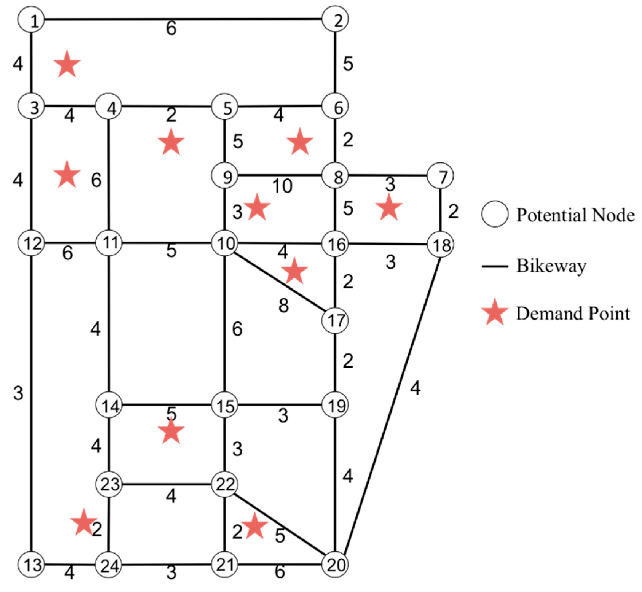
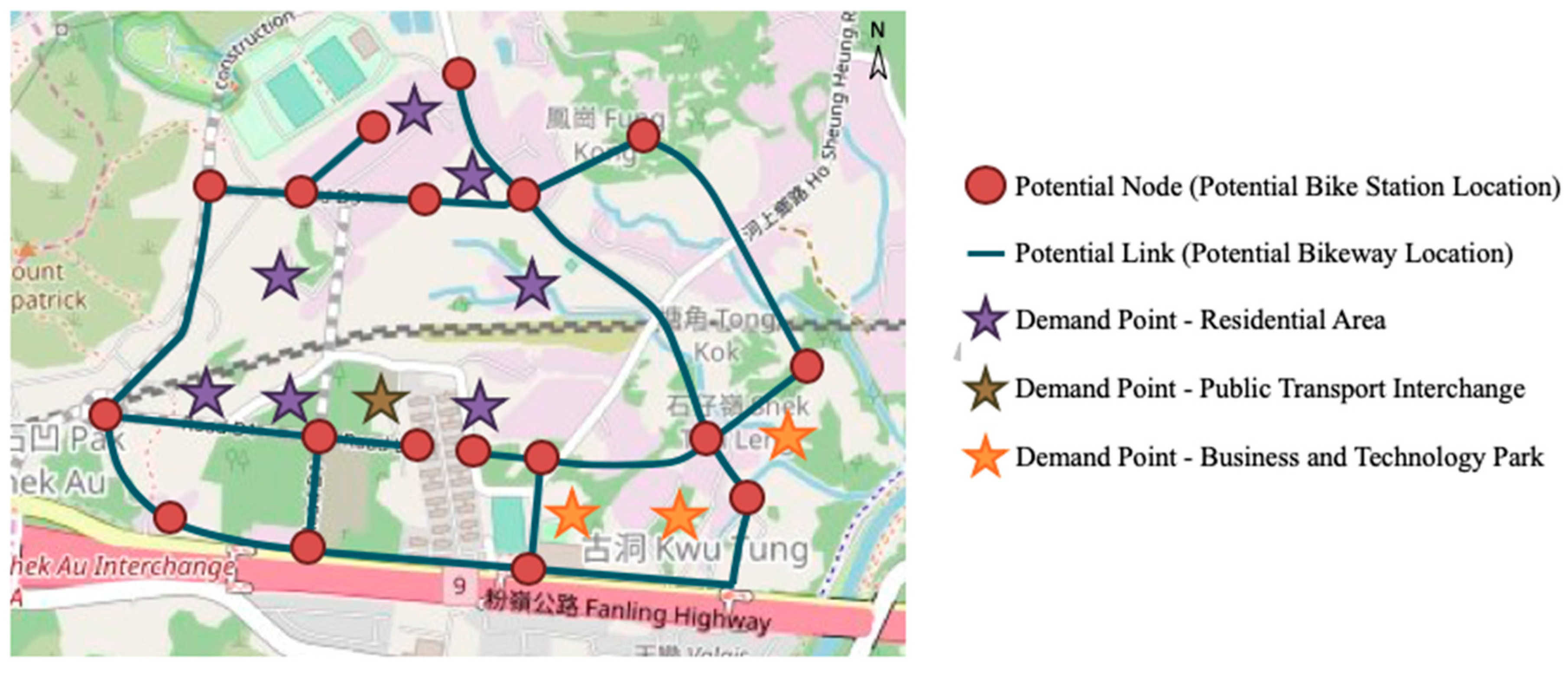
The design problem is described below. We firstly consider a potential bikeway network G(V, E) with potential bike station location (i.e., node) set V, potential bikeway set E, and demand point set D. The total demand traveling from point k to point l is denoted as $d_{kl}$, where $k,l\in D$, and each bikeway that directly connects stations i and j, i.e., $e_{ij}\in E$, has the setup cost $c_{ij}$ where $i,j\in V$. The travel time $t_{ij}$ between the nodes can be different with respect to the travel direction to consider the case that the bikeway is built on a slope. In other words, the downhill travel time can be greatly reduced compared to the uphill travel time. Each demand point $k\in D$ is considered as “covered” when there is at least one proximate bike station for convenient bicycle pick up/ drop off (which should be less than 500 m, as revealed by reference [20]). This defines $M_k$ as the set of potential bike stations which are proximate to demand point k, where $M_k\subset V$. It is also assumed that every demand point is covered by at least one potential bike station (i.e., $\nexists M_k=\varnothing ,\forall k\in D$). The budget for the total bikeway construction is set to be B. For simplicity, all potential bike stations are assumed to have unlimited capacity.

This design problem involves two types of design decisions. The first type is to determine whether a node is picked as a selected node, denoted by a binary decision variable $X_i$ which equals 1 if node i becomes a selected node and 0 otherwise. A selected node is defined as a node that covers at least one demand source and is connected by at least one bikeway. To separate the selected nodes from the unselected nodes, all selected nodes are put into a new set S, where $S\subset V$. The second type is the binary decision variable for opening a bikeway $Y_{ij}$, which equals 1 if the bikeway that connects nodes i and j is constructed and 0 otherwise. An additional note is that we have assumed that every built bikeway has sufficient capacity to accommodate all bike flows and thus the travel time can be a flow-independent constant. In other words, if the bikeway travel time is flow-dependent, a possible extension is to include the third type of decision variables, flow on each bikeway, in the design problem.

This problem involves determining the bikeway layout under four following conditions: (a) the total travel times of all cyclists is minimized, (b) all demand points are covered, (c) all selected node pairs are connected by bikeways, and (d) the total bikeway setup cost does not exceed the budget.

The design objective based on condition (a) can be expressed as

$$\min {\displaystyle \sum }_{i\in S}{\displaystyle \sum }_{j\in S}{d}_{ij}{T}_{ij}.$$

(1)

where $T_{ij}$ denotes the lowest travel time between stations i and j based on the constructed bikeways, where $i,j\in S$. For the demand between points k and l, $d_{kl}$, the shortest path is determined among a maximum of $\left|M_k\right|·\left|M_l\right|$ possible paths formed by the potential bike stations close to these two points. Among these paths, the shortest path is the one that has the minimum travel time and the origin and destination of the path are selected nodes. When both points share the same selected node, the travel time between the nodes becomes 0. When there are multiple shortest paths with respect to time between a pair of selected nodes, all demands are assigned to the path with the lowest setup cost. As a result, all demands of a pair of selected nodes are only assigned to a single shortest path.

Proposition 1.

For every feasible solution to the problem, there exists at least one path between every pair of demand sources.

Proof. 

Condition (b) implies that at least one bike station proximate to a demand source is a selected node to cover all demand points. Thus, both the origin and the destination of every pair of demand sources have been covered by the selected node. From condition (c), every pair of selected nodes must be connected by at least one path. Therefore, there must be at least one path between every pair of demand sources and this completes the proof. □

Condition (b) (i.e., demand coverage constraint) is satisfied when all demand points are covered by at least one selected node, which can be expressed as

$${{\displaystyle \sum }}_{i\in M_k}{X}_i\ge 1,\forall k\in D.$$

(2)

Constraint (2) ensures that at least one potential bike station proximate to each demand point is a selected node. The connectivity between the selected nodes (i.e., conditions (c)) is hard to be expressed solely by $X_i$ and $Y_{ij}$ as the paths between the selected nodes can involve links that consist of unselected nodes. Unlike the minimum spanning tree, we can neither exclude cycles nor set exact bounds to the number of links because the final network layout is unlikely to be tree-like. The connectivity condition can, therefore, be described by the following set of necessary but not sufficient conditions: first, each selected node is connected by at least, but not exactly, one bikeway; and second, the two ends of an opened bikeway can be both unselected nodes.

Finally, condition (d) can be formulated as the total bikeway setup cost cannot exceed a given budget B, which can be expressed as

$${{\displaystyle \sum }}_{i\in V}{{\displaystyle \sum }}_{j\in V}{c}_{ij}{Y}_{ij}\le B.$$

(3)

As the problem contains the complicated connectivity constraint which cannot be expressed mathematically, metaheuristics should be adopted to solve the problem.

3. The Two-Stage Solution Method

This section presents a two-stage solution method to solve the proposed problem. A genetic algorithm (GA) is adopted firstly to determine the optimal selected node set, and a proposed elimination heuristic (EH) determines the optimal bikeway layout that minimizes the total travel cost without violating the budgetary constraint based on the selected node set.

3.1. The Genetic Algorithm

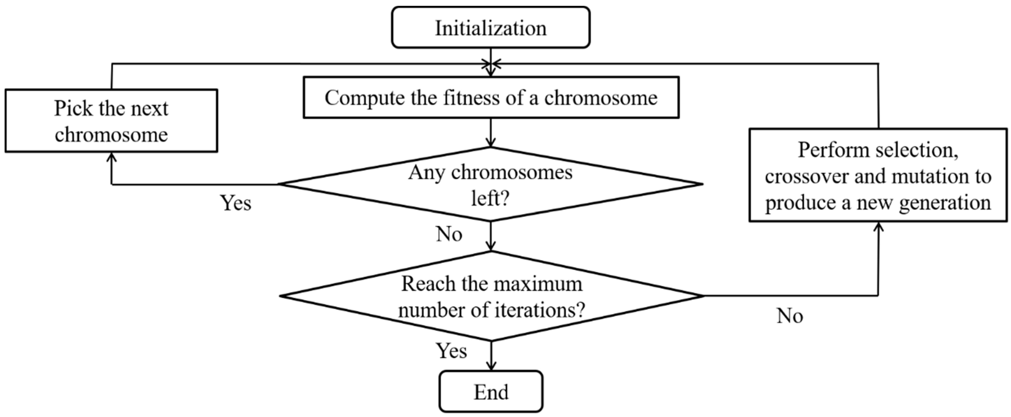
Figure 1 illustrates the general scheme of the GA for determining the optimal node set. At first, a population of solutions is initialized randomly, in which each individual (solution) in GA is represented by a chain of binary digits with length |V| (number of potential stations). The number of ‘1’s on each chain can be interpreted as the selected nodes of that solution. After evaluating the fitness of all initial solutions, the truncation selection method is adopted to select the x% of the fittest parents in the population and duplicate $1/x\%$ times to replace the less fit parents. For example, when the fittest 50% of parents are selected from a population of 100 individuals, the selected parents are duplicated 2 times so that a population of 100 individuals can be maintained. Then the parents would have a certain probability of undergoing crossover and mutation for generating new offspring. In the crossover, a crossover point along the chain is randomly selected, and all digits beyond that point are swapped between the two parents. In mutation, a random position in the solution is picked for flipping the bit at that position (as each position can be either 0 or 1). After the crossover and mutation processes, the solutions are compared to remove replicated solutions. Meanwhile, an elitist selection is carried out in GA by storing the best solution from the current generation to be carried over to the next iteration without alteration. The above process is repeated until the maximum number of iterations is reached.

Every generated solution needs to undergo a three-stage solution fitness evaluation. The first stage is a demand coverage check that verifies whether the selected nodes can cover all demand sources. The solution is regarded as infeasible if the selected nodes cannot cover all demand points: its fitness is not further evaluated and a large penalty is imposed. In contrast, a selected station set that can cover all demand points is regarded as feasible and its fitness is then evaluated by the elimination heuristic. The second stage is used to evaluate if the cost of the bikeway network falls below the budget. The elimination heuristic (introduced in Section 3.2) aims to determine a feasible bikeway layout for a given selected node set (from stage 1) which connects all selected nodes and does not exceed the budget. If all selected nodes cannot be completely connected under the given budget, the selected node set is also classified as infeasible, and a smaller penalty (compared with the penalty for demand coverage) is imposed on that infeasible node set. After screening out the infeasible solutions, the third stage is to determine the objective values (total system travel times) of the remaining feasible solutions, and the solution fitness can be calculated as the reciprocal of the objective value.

3.2. Elimination Heuristic

The EH is applied to every selected station set which covers all demand points (determined by GA) in order to determine a feasible bikeway layout that does not violate the budget constraint. The steps of the EH are as follows:

Step 1

Obtain the network G_F with the shortest paths between all pairs of selected nodes E_F. Terminate if budget B is not exceeded.

Step 2

Assign an elimination factor $f_{ij}$ to each link $e_{ij}$ in G_F according to its path count $p_{ij}$ and cost $c_{ij}$. List and sort the links in descending order $f_{ij}$.

Step 3

Remove the link with the largest $f_{ij}$ in the list and evaluate the network connectivity. Undo the link removal if the selected nodes become disconnected.

Step 4

Remove the evaluated link from the list.

Step 5

Repeat Step 3 until the cost is equal to or lower than B. If the cost is still higher than B after removing all possible links, a penalty is given to the selected node set to denote the solution infeasibility.

Step 1 is to construct a network G_F(V_F, E_F) which consists of the node set V_F and path set E_F, in which V_F and E_F correspond to the selected node set S and the set of shortest paths between the selected node pairs respectively. To determine E_F based on the original network G(V, E) and S, this study applies the minimum spanning tree algorithm (with respect to travel time) for |S| times. The information of all shortest paths between all pairs of selected nodes (e.g., total cost, total travel time, and links included in the path) is then determined and stored. In other words, all selected nodes can reach other selected nodes with the lowest travel times. At this stage, the resultant bikeway network at this step has the lowest total system travel time and the highest total construction cost as most bikeways are constructed.

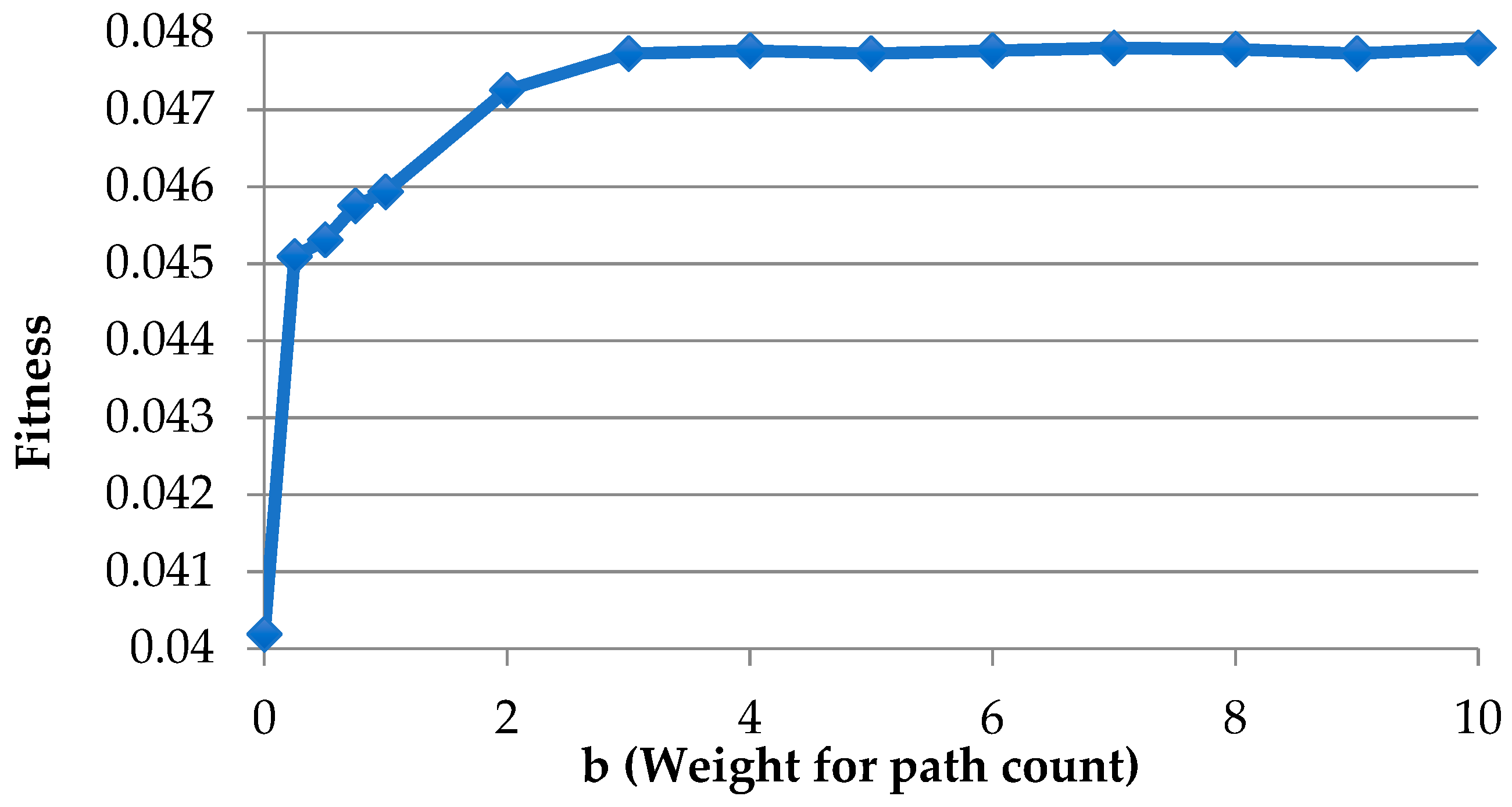
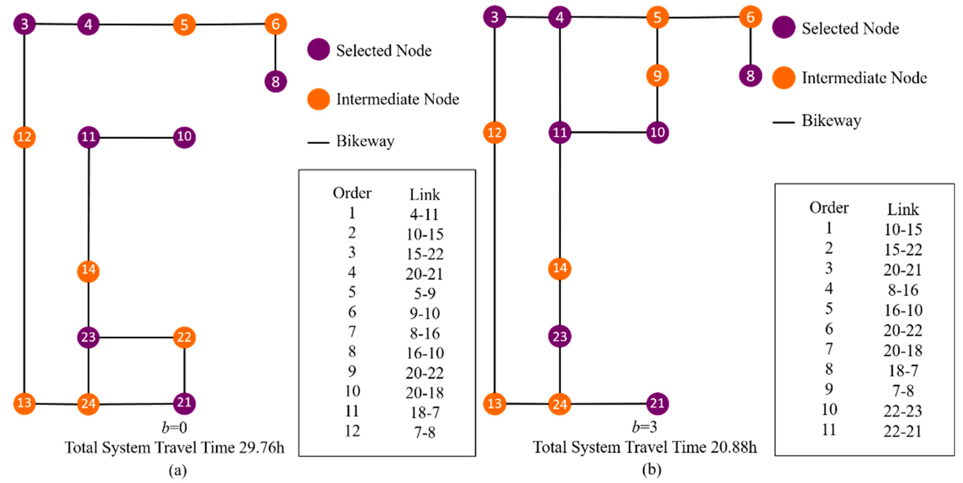
Step 2 is to determine the order of elimination of the built bikeways given in Step 1 by using the elimination factor $f_{ij}$ to meet the budget constraint. The link-based factor is composed of two parts, the construction cost $c_{ij}$, and the path count $p_{ij}$, and expressed as $f_{ij}=a·c_{ij}+b/p_{ij}$, where a and b are the non-negative weights for the cost and reciprocal of the path count, respectively. Path count describes the number of shortest paths using the link which can be determined based on the stored path information in Step 1. In other words, links that have higher costs or fewer shortest paths have a larger elimination factor, which implies higher chances to be eliminated. Using this factor is better than simply removing links with respect to cost because it avoids removing high-cost links used by a large number of shortest paths. For simplicity, the elimination factors of all links remain unchanged throughout the evaluation of each solution. In addition, the bikeways which perform as the only link that connects the selected node with other nodes are automatically removed from the list despite a low path count or a high construction cost.

Step 3 evaluates the connectivity between the selected nodes to determine whether any selected node pairs have been permanently disconnected after each bikeway removal. Instead of reconstructing all paths E_F, this step focuses on checking those paths that include the removed link. The heuristic determines whether the two ends of the removed link can be connected by a new path using other built bikeways. If they cannot be connected, the removed link is restored; if they can be connected, the travel times of those affected paths are updated.

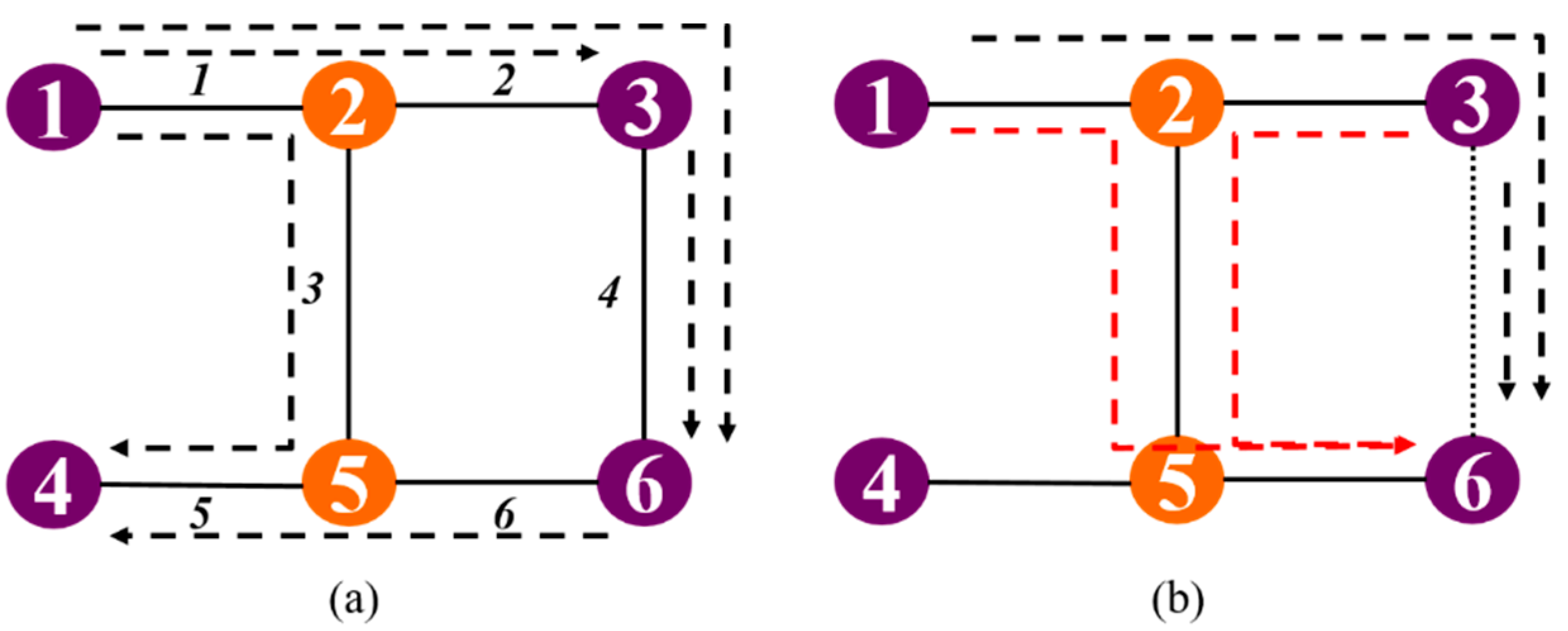
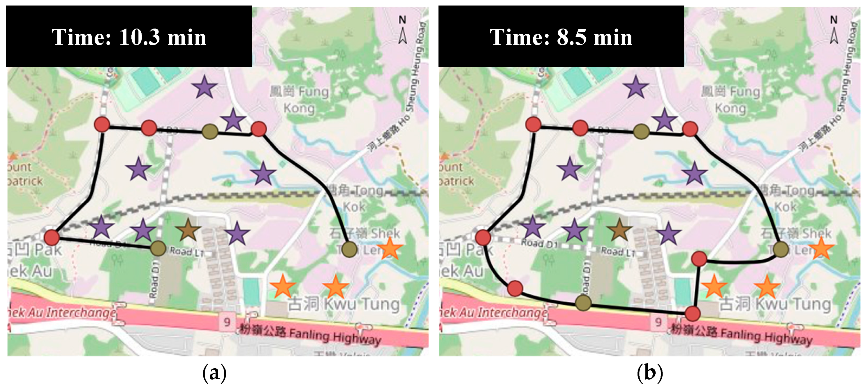
The calculation of the updated travel time is not equivalent to the simple addition of the difference in travel time between the new path and the removed link, which can be explained by an example shown in Figure 2a,b. In these figures, nodes 1, 3, 4, and 6 are the selected nodes while nodes 2 and 5 are not. The solid lines denote the built bikeways, the black dotted lines with arrow denote the shortest paths between the selected nodes, and the italic numbers denote the link number. Figure 2a,b show that the initial shortest paths between the selected nodes and the case after link 4 is removed, respectively. When link 4 is removed (in Figure 2b), two shortest paths (between nodes 3-6 and nodes 1- 6) need to be re-routed and the updated shortest path between nodes 3 and 6 becomes 2-3-6. Meanwhile, if this updated shortest path sequence between nodes 3 and 6 is directly substituted into the original shortest path between nodes 1 and 6 (i.e., 1-2-4), the shortest path becomes 1-2-2-3-6 that link 2 is visited twice consecutively which shows a redundant visit on link 2. Therefore, the updated shortest path between nodes 1 and 6 should completely remove the duplicated links and thus becomes a path with link sequence 1-3-6.

Based on these two cases, the network connectivity evaluation and path updates follow the following steps:

Step 3.1

Determine the new shortest path W that joins the two ends of the removed link V and store its link sequence.

Step 3.2

Update the shortest paths in E_F that contain V by directly substituting I with W.

Step 3.3

Determine the updated travel time T’ and link sequence of each shortest path following the below rules:

(a)

If it has no duplicated link, then T’ is the sum of the original travel time and the travel time difference between V and W, and the updated link sequence is obtained by simply substituting V with W.

(b)

If there are duplicated links, T’ is calculated by firstly following Step 3.3(a) and then subtracting two times the sum of the duplicated links along the route, and the duplicated links are removed from the link sequence of the updated shortest path formed in Step 3.2.

After removing a link, the path counts of all built bikeways are updated and the built bikeways with zero path count are then immediately removed from the list.

Finally, Step 5 is the termination criteria of the EH in which the heuristic stops only if the total setup cost is lower than the given budget. To distinguish the infeasible solutions with the feasible ones, a large penalty is imposed when the network connectivity is not conserved. This gives preferences to the all-connected networks instead of disjoint networks.

4. Numerical Results

The numerical studies aim to (1) investigate the effect of the weights for elimination factor, (2) analyze the effect of the budget on the total system travel time and the solution fitness, and (3) examine the effect of the number of demand points on the construction cost. The proposed solution method was coded with Dev-C++ and ran on a computer with 3.40 GHz and 6.00 GB of RAM. The GA has a population size of 30 with a 50% truncation rate, a 40% crossover rate, and a 60% mutation rate.

4.1. Effect of the Weights in the Elimination Factor

The solution quality relies strongly on the elimination factor f_ij. The weights for the elimination factor, a (for the cost) and b (for the path count), should be calibrated to avoid overemphasizing either attribute. In the experiments, the genetic algorithm was run with the Sioux-Falls network (see Figure 3). To fit our test problem, nine demand sources are added to the network. The weight for the cost a was kept at 1, while the weight for the path count b varied from 0 to 10. Figure 4 shows the effect of the weight of path count on the solution fitness. The solution fitness improves significantly when b increases from 0 to 0.25, improves slightly from 0.25 to 3, and remains steady with negligible fluctuations when b is greater than 3. The values of a and b are thus set to 1 and 3, respectively, in the following sections.

Figure 5 shows that the solution fitness changes with the value of b because the weights for the elimination factor change the order of link elimination and thereby affect the network layout. To study the sole effect of the value of b on the solution fitness, the two networks in Figure 5 use the same selected node set with different values of b (i.e., 0 and 3). The results show that the network in Figure 5b has a lower total system travel time than that in Figure 5a, given that both networks do not exceed the budget constraint, mainly because of the differences in the order of link elimination. For example, the high-cost link 4-11 is eliminated immediately when path count is not considered (i.e., b = 0). Nevertheless, it is kept when the path count is considered because its high path count lowers its order of link elimination. When this link is kept, the shortest paths which use link 4-11 do not have re-routing and thus a lower total system travel time can be achieved. This shows that the elimination factor can be a better approach than cost-based elimination in lowering the total travel time.

The difference in the value of b can result in different selected node set and thus the network layout.

Table 2. Solution fitness under different values of b.

Value of b	0	1	2	3
Size of selected node set	7	7	7	7
Solution fitness	0.04371	0.04664	0.04771	0.04771
Total travel time (hr)	22.88	21.44	20.96	20.96

lists the details of the optimal network layouts with different values of b. While all networks have 7 selected nodes, there are two different selected node sets and three different network layouts. For b = 0, its selected node set of b = 0 is identical to the sets of b = 2 and 3 but the resultant network layout has a higher total system travel time. The eliminated links when b = 0 are different from those when b = 2 and b = 3 due to the difference in the elimination factor of the links and thus due to the order of elimination. For b = 1, the network layout is different from the layouts when b = 2 and 3 due to the difference in the selected node set, so as the eliminated links. When b = 2 and 3, the selected node set and the network layout are identical and the total system travel time is the lowest possible. This shows that the path count can also influence the selected node set and thus the total system travel time.

4.2. Effect of the Budget on the Solution Fitness

This section demonstrates the trade-off between the budget and the solution fitness (as well as the total system travel time) via two cases. The first case adopts a fixed selected node-set consisting of 17 selected nodes from the network illustrated in Figure 3, and it is assumed that the selected node-set covers all the demands. With a defined selected node set, the elimination heuristic was solely used to evaluate the network layout and the total system travel time with different budgets. Figure 6 illustrates that the solution fitness increases when the budget increases, which is consistent with the intuition that a higher budget can construct more bikeways and thus reduces the total system travel time. When the budget is lower than 64, no infeasible solutions can be obtained as at least one pair of selected nodes is unconnected. When the budget equals 64, the bikeway layout is indifferent from the Steiner tree network in which the selected nodes are connected with minimal construction cost. This network has the highest total system travel time because most bikeways that contribute to some of the shortest paths are eliminated to minimize the cost, and therefore those selected node pairs have a longer travel time. On the other hand, the bikeway network has the lowest total system travel time when the budget is at or above 139. At this budget level, all shortest paths between all selected node pairs can be constructed. The minimal total travel time is achieved because all cyclists can travel on the corresponding shortest paths. Furthermore, when the budget increases from 64 to 139, there exist network layouts other than the Steiner tree and all shortest paths’ network (as shown in Figure 7). While the budget is in between the upper and lower bounds, these networks have a lower total travel time than the Steiner Tree but a higher travel time than the all-to-all shortest path network. This shows the capability of the elimination heuristic in determining the budget-constrained solutions under the objective of travel time minimization. The existence of intermediate solutions between the solutions of the Steiner tree problem and the Floyd-Warshall algorithm also implies that the design of the bicycle network is sensitive to the budget. As the elimination heuristic can find these intermediate solutions, it allows the planners to use the budget as a parameter to design the bicycle network. The bicycle network obtained by the elimination heuristic can always meet the budget while minimizing the total system travel time.

In the second case, the selected node set is not predefined, but it needs to satisfy the demand coverage constraint. Unlike the first case, the budget level can alter the sets of selected nodes. Figure 8 shows that the solution fitness increases with the budget, which is consistent with the previous results. When the budget is lower than 42, all obtained solutions are infeasible because the built bikeways are insufficient to cover all the demand points. Figure 9 displays the network layout with a budget of 35. Some demand points are uncovered because the budget is not sufficient for building bikeways to connect all of their proximate stations. These results show that this model can determine whether the budget is enough for a feasible design and provide different designs according to the given budget.

4.3. Effect of Number of Demand Points on Construction Cost

This section investigates the effect of the number of demand points on the construction cost. Different numbers of demand points were inputted into the model, and the minimum cost for covering all demand points was then obtained. The example network is identical to that in Figure 3. Figure 10 shows the relationships between the number of demand points and construction cost.

Figure 10 shows that the construction cost increases with the number of demand points. In general, more demand points require more selected nodes to cover all demands. As a result, more bikeways are constructed to connect these selected nodes, and the construction cost increases. Figure 11 illustrates how the number of demand points affects the number of selected nodes and thereby the construction cost. This figure also indicates that the budget amount affects the maximum number of covered demand points. When the budget is tight, only a few demand points can be covered. In this case, we should carefully investigate the relative importance of the demand points so that we can decide which demand points are worth to cover. In contrast, when the budget is higher, more demand points can be covered so as to increase the coverage of the bikeway network.

5. Application in Hong Kong

This section aims to show the application of our model in Hong Kong. Two case studies were carried out in Kwu Tung North and Kam Tin (i.e., two proposed new towns in Hong Kong) to illustrate how our model can be applied to develop a new bicycle network and improve the existing network in Hong Kong. Developing a bikeway network coincides with the aim of the Hong Kong government in promoting cycling in new towns and development areas for short-distance commuting [21], in which the government has launched several projects that connect scattered cycle tracks in the New Territories and creates new bicycle networks in tourist spots [22]. Our proposed model can be useful to design the bikeway network in Hong Kong due to three reasons. First, it ensures popular destinations (e.g., public transport interchanges or tourist spots) to be covered by bikeways and interconnected. This is unlike the existing networks where the bikeways connect unpopular locations and thus many of them go unused [23]. Second, this model focuses on a network design with continuous and exclusive bikeways, which is favorable to the vast majority of inexperienced cyclists in Hong Kong who only cycle in a safe cycling environment. Thirdly, this model aims to minimize total travel time under the given budget, which is useful for the government that often has a fixed budget for bikeway construction.

5.1. Design Parameters

The unit cost of all bikeways is assumed to be the same, which is taken as c = HK$630 per meter, despite the construction materials, foundation, and technology applied [23]. The cost of building a bikeway between nodes i and j would be $C_{ij}=c\times l_{ij}$, where l_ij is the distance between nodes i and j. The distance l_ij would also be used for calculating the travel time between the bike stations. It is assumed that the cyclists travel at v = 20 km/h by bike [20]. The travel time between nodes i and j would be $t_{ij}=l_{ij}/v$.

5.2. Case Study in Kwu Tung North

Kwu Tung North (KTN) is one of the new development areas in the North East New Territories. It is planned to be 447 ha and to be developed as a mixed development node [24]. As the government aims to provide a quality living environment, a bicycle network will promote cycling within the area. Since there are no existing cycle tracks in KTN, we can demonstrate how our model designs a completely new bicycle network in this area. All the maps were obtained from OpenStreetMap [25], while the potential links and demand points have been identified from the Statutory Planning Portal of the Town Planning Board, Hong Kong [26]. We selected the residential area, the public transport interchange, and the business and technology park to be the demand points, as shown in Figure 12.

Figure 13a,b show the bikeway layouts under different budget levels. With a higher budget level (i.e., Figure 13b), the bikeways are denser and the total system travel time is reduced, which is consistent with the numerical results in Section 4. As shown in Figure 13a,b, a higher budget results in a larger number of selected nodes that are located closer to the demand sources and a longer continuous bikeway. From these results, we can conclude that our model can be applied to design a bikeway network in new development areas. The model is particularly useful when the government has a fixed budget, as it can guarantee a below budget design that minimizes the cyclists’ total travel time.

5.3. Case Study in Kam Tin

The government has planned a new residential development in Kam Tin (KT) South to increase the local housing supply [27]. The existing bicycle network should be expanded so that the new residential area can be connected to the Kam Sheung Road Station (KSRS). Meanwhile, there are only a small number of cycle tracks and parking sites in KT as shown in Figure 14. To facilitate cycling in KT, more cycle tracks and parking sites should be built. Figure 14 shows the demand points and the network. It is noted that some roads are not chosen as the potential bikeway locations because they are either too narrow or are owned by private owners.

Figure 15a,b display the final bikeway network layouts under different budget levels. In this case, provided that there are existing bikeways and parking sites, the model was modified to ensure that these existing facilities are not removed in the elimination heuristics. The results of the bikeway designs are consistent with other sections that the total system travel time decreases when more budget is provided. Also, the travel time between the existing bike stations/ parking sites can be reduced because the stations can be connected by a shorter path when more budget is provided. These results show that our model handles the case of system expansion in which the new design can improve the system performance while taking the existing bicycle network and given budget level into consideration.

6. Conclusions and Future Directions

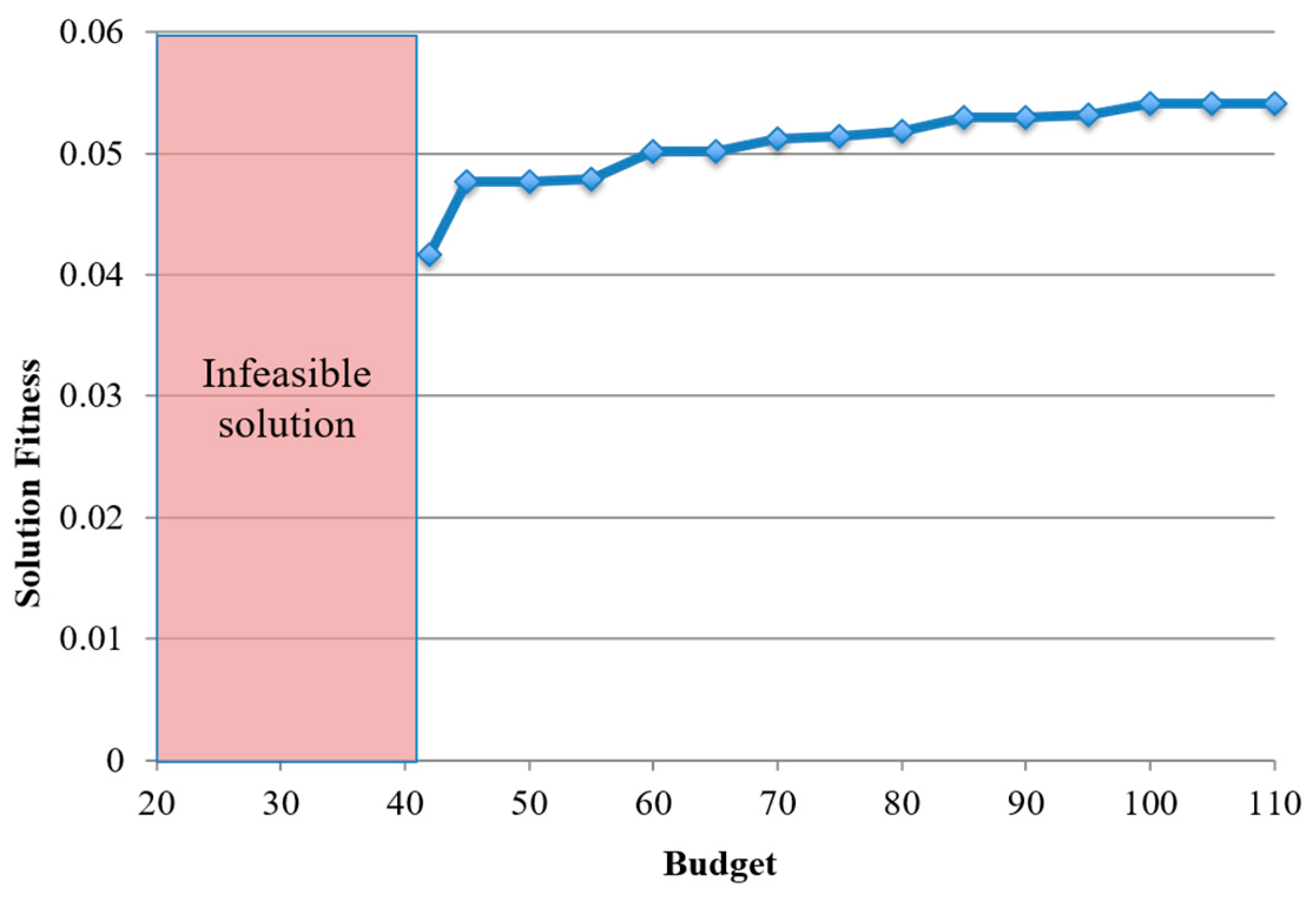
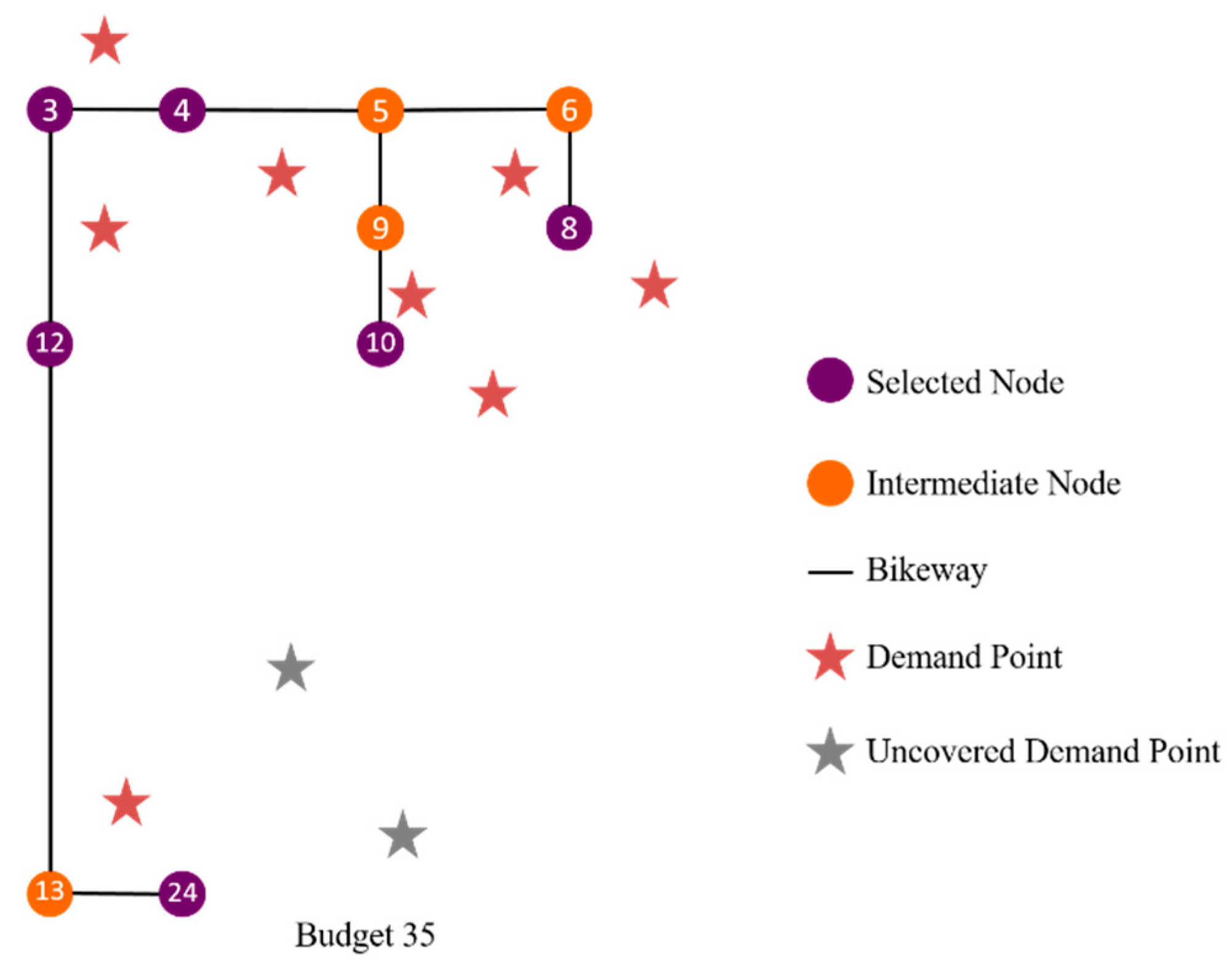
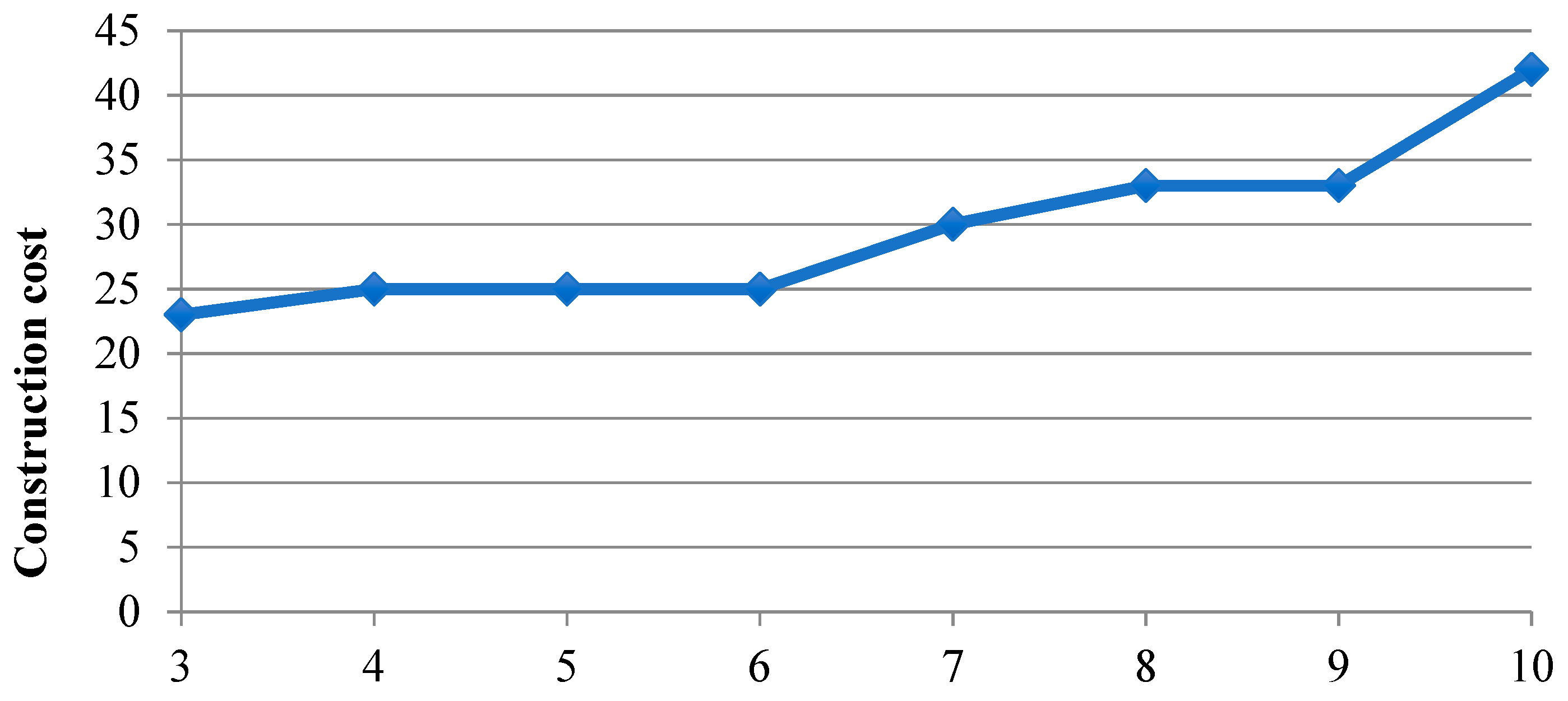
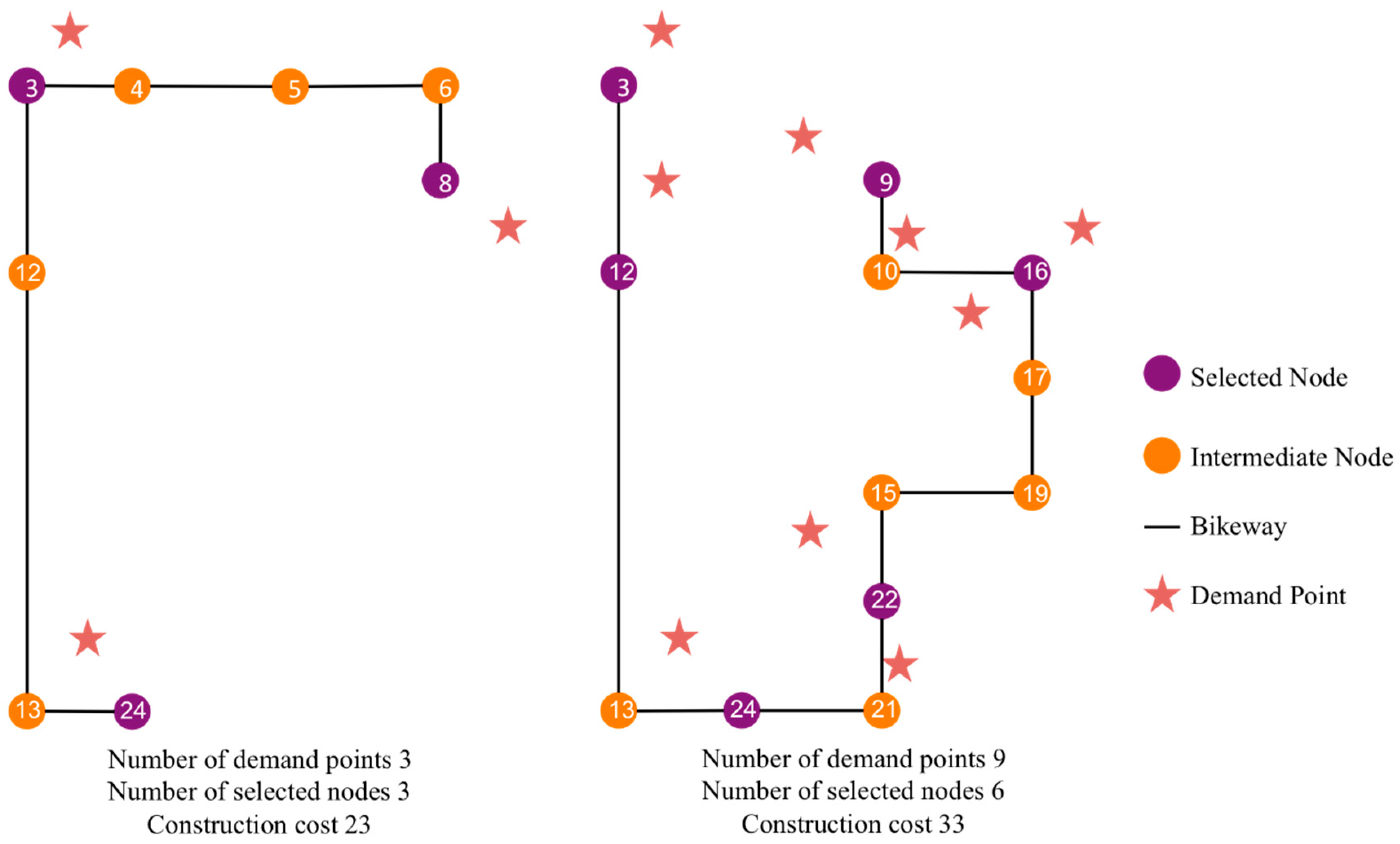
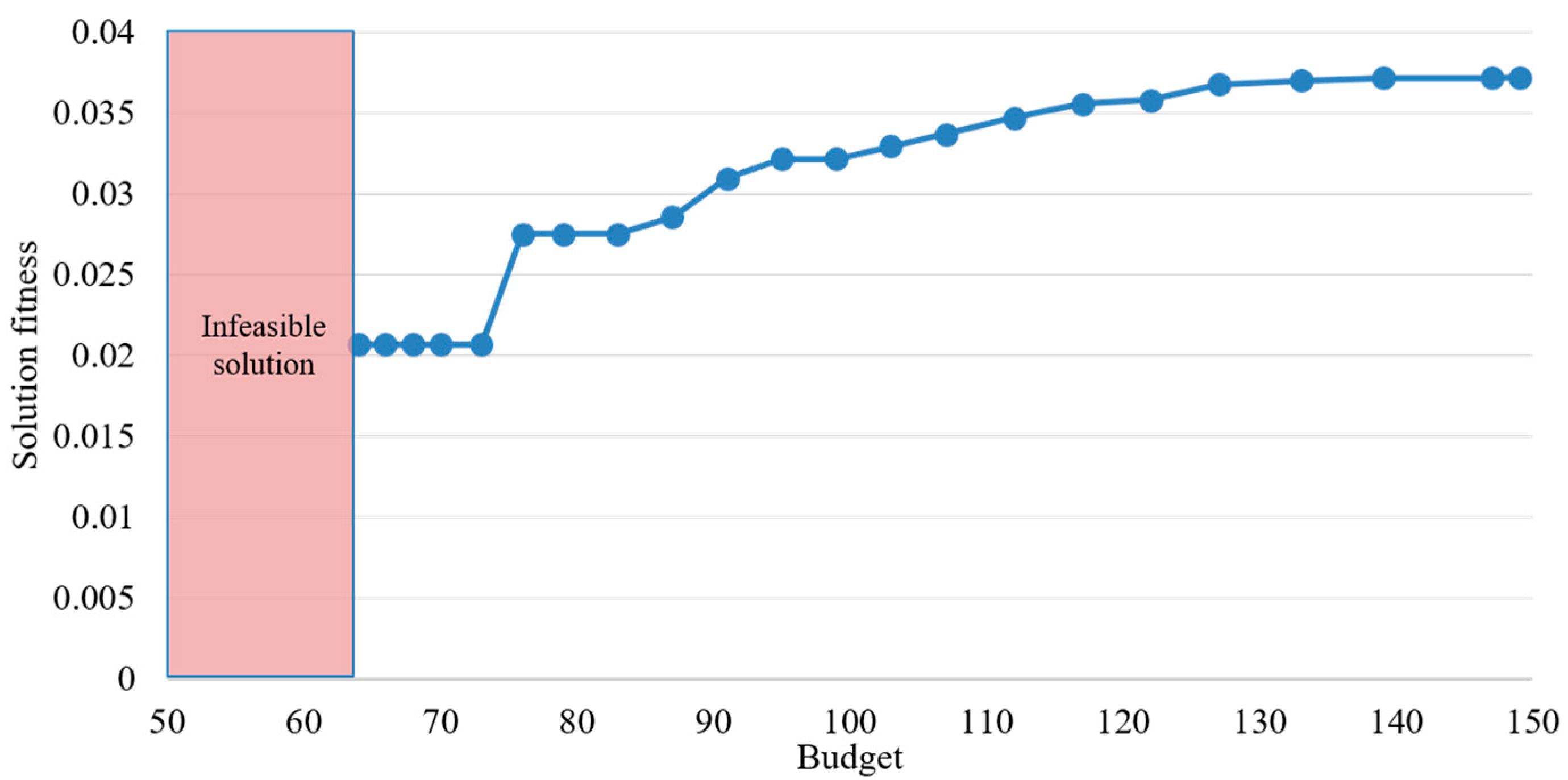
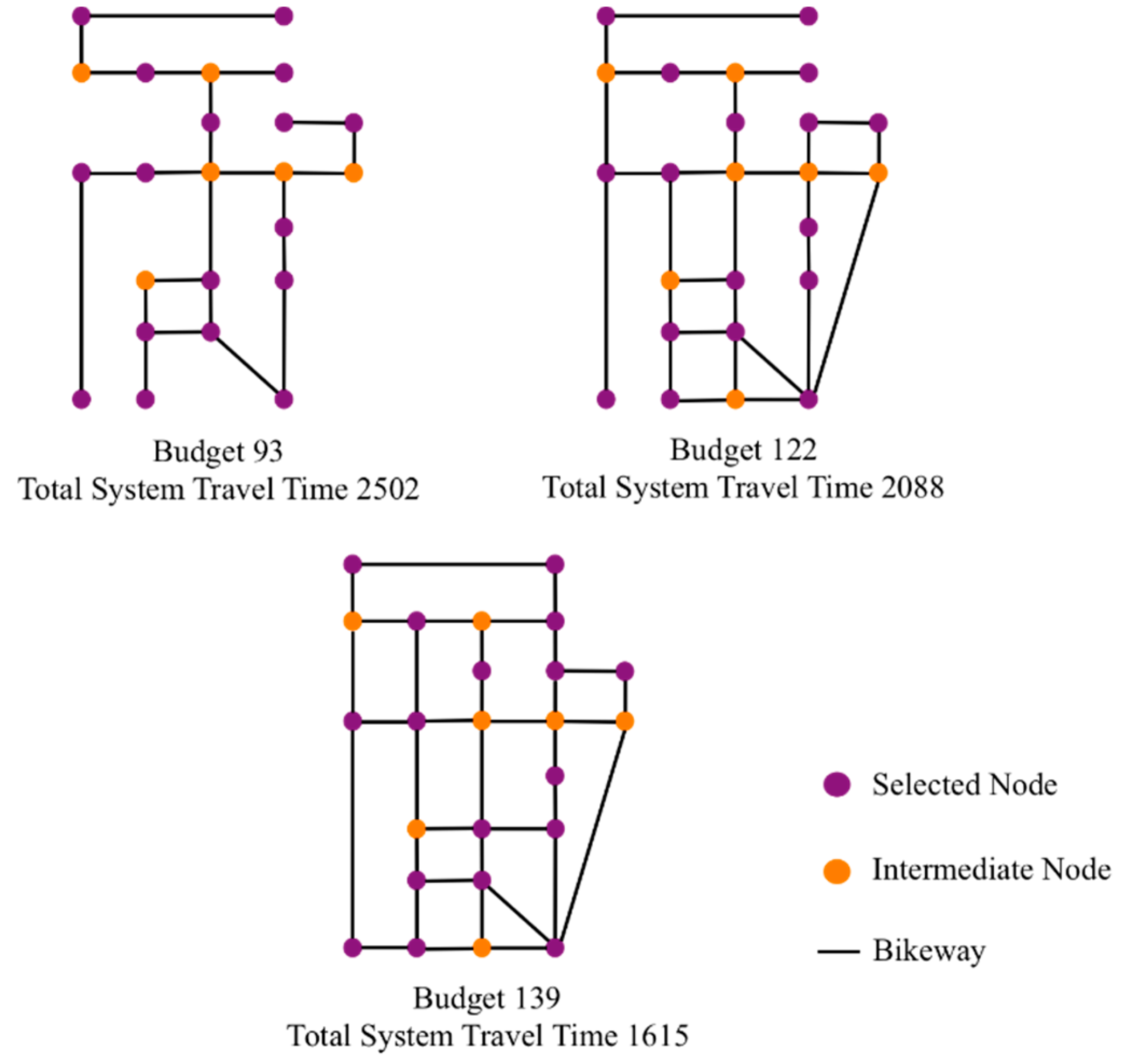
In spite of the significant role of bikeway in motivating cycling, there are very few existing bikeway network design models, and some design objectives and constraints have not been simultaneously taken into consideration. This study proposes a new bikeway network design problem that minimizes the total system travel time between a set of selected nodes under a budget constraint, in which all potential demands must be covered by the selected nodes and all selected nodes must be interconnected. An efficient two-step solution method is proposed to determine the selected node set and the bikeway layout separately. The genetic algorithm is employed to determine the selected node set that covers all demand points, while a novel elimination heuristic is employed to remove the bikeways between the shortest paths of the selected nodes (constructed by the shortest path algorithm) according to the elimination factor (which is a weighted sum of the setup cost and path count). Numerical studies showed that (1) the weights for elimination factors can significantly change the network layout and thus the solution quality; (2) a higher budget can change the network topology and improve the solution fitness whenever the selected node set is fixed or flexible; and (3) the construction cost increases with the number of demand points. The case studies in two Hong Kong new towns showed that the model can handle design problems with or without existing bikeways under various budget levels. This model can, therefore, be adapted to similar bike-sharing system designs because (1) it ensures that the resultant bike station locations have complete demand coverage, (2) all bike stations can be well-connected by the bikeway network, and (3) the designed network can satisfy the budget constraint. Furthermore, the model is not only applicable to new system designs but can also capture the existence of built bikeways and bike stations for system expansion.

Future research could be done in the following directions. First, other design constraints or measures, such as BLOS, could be included in the model. Second, the model assumes that the demand between every demand point pair is identical, while it can be relaxed in future studies by considering varying demand levels of all demand sources, elastic travel demand with respect to travel time, or uncertainties between the selected nodes. Third, the bikeway setup cost is assumed to be proportional to the length of links only, but it can also be influenced by other factors, such as the type of bikeway (e.g., exclusive bikeway, shared bikeway with vehicle roadway) and pavement type. Future studies can be extended to multi-type bikeway design problems. Fourth, the generalized travel cost of each bikeway can include other attributes in addition to travel time, including the number of turns and intersections, the percentage of greening, and the provision of cycling facilities along with a candidate link. Moreover, the route choice behavior of the cyclists can be remodeled by including other route choice attributes (such as traffic flow of automobile on the edges) or using other mathematical forms such as the bi-objective model [28]. Finally, the Genetic Algorithm used in the two-stage solution method can be replaced by other new meta-heuristics or hybrid meta-heuristics, such as the Artificial Bee Colony algorithm, Tabu Search, or Large Neighborhood Search. Comparative studies can be carried out to determine which of the solution methods has a higher computation efficiency.