Combining Multi-Modal Statistics for Welfare Prediction Using Deep Learning

Abstract

In the context of developing countries, effective groundwater resource management is often hindered by a lack of data integration between resource availability, water demand, and the welfare of water users. As a consequence, drinking water-related policies and investments, while broadly beneficial, are unlikely to be able to target the most in need. To find the households in need, we need to estimate their welfare status first. However, the current practices for estimating welfare need a detailed questionnaire in the form of a survey which is time-consuming and resource-intensive. In this work, we propose an alternate solution to this problem by performing a small set of cost-effective household surveys, which can be collected over a short amount of time. We try to compensate for the loss of information by using other modalities of data. By combining different modalities of data, this work aims to characterize the welfare status of people with respect to their local drinking water resource. This work employs deep learning-based methods to model welfare using multi-modal data from household surveys, community handpump abstraction, and groundwater levels. We employ a multi-input multi-output deep learning framework, where different types of deep learning models are used for different modalities of data. Experimental results in this work have demonstrated that the multi-modal data in the form of a small set of survey questions, handpump abstraction data, and groundwater level can be used to estimate the welfare status of households. In addition, the results show that different modalities of data have complementary information, which, when combined, improves the overall performance of our ability to predict welfare.

1. Introduction

Sustainability is a multidimensional and dynamic problem where the most severe challenges often exist in the places with the least data. In rural Africa, the imperative for economic development and poverty reduction is constrained by the variability and uncertainty in environmental systems. Groundwater is the most widely available, water resource but it is poorly quantified in terms of its availability in locations where bulk water users, such as irrigated agriculture or mining, may influence and impact the use and quality for rural populations for drinking water or other household needs. We explore how machine learning methods can fuse multiple streams of biophysical and social data to understand and predict how the multidimensional welfare of people may be at risk from the temporal and spatial variation in the use and distribution of groundwater in coastal Kenya. If the status and changes in groundwater and welfare risks can be quantified this will permit policy and investments to find and maintain a more sustainable balance between the competing goals of economic growth, environmental sustainability and poverty reduction.

1.1. Contributions of This Work

In this work, we employ a deep learning-based method to estimate the welfare status of households using multi-modal data. Deep learning is a type of machine learning method based on artificial neural networks (ANN) [1]. Machine learning is the scientific study of algorithms and statistical models that can automatically detect patterns in data and use them to perform certain decision task [2]. In ML we model the relationships within the input modalities of data with its output and they perform a certain task relying on the patterns and inferences without using any explicit instructions. The final output of the ML model incorporates both dynamical trend information and subtle correlations that may exist between the various input modalities of the data. ANN derive their inspiration from the working of biological neurons. Deep learning employs multiple layers of ANN to build a model which progressively extract patterns from the input signal. Deep learning allows the output of the model to cope with signals that are sampled at different times, and corrupted by varying degrees of artefact and noise. DNN can also scale to the modeling of very large quantities of big data in a principled manner, where model structure is learned directly from the data. Compared to prior deep learning-based studies, the proposed work differs in two key ways: (1) with a primary motivation to generate data and tools required to inform policies, interventions and investments related to drinking water management, we focus on predicting the welfare status of people specifically with respect to drinking water resource, and (2) our model combines household level socio-economic survey data with two other modalities of data such that the welfare can be modeled with respect to their proximal drinking water resource. We use a deep neural network and compare results with traditional machine learning methods. The importance of individual modality is analyzed and it is observed that combining them improves performance.

1.2. Background

A reliable estimate of the welfare of people is important to inform a country’s development policies, even more so for countries with constrained resources. Such information allows government to efficiently allocate its resources and track progress of development activities. Nevertheless, many countries lack the data and the tools required to monitor their resources and how they link to the welfare of people [3], which substantially affects their ability to focus more on the areas or populations with the highest need [4,5]. The welfare data of a population is generally collected using socio-economic surveys consisting of a detailed questionnaire, which are often time consuming and resource-intensive. Often these survey datasets are not in the public domain and have limited coverage [6,7]. Despite recent global push to ramp up data collection within developing nations [3], the use of traditional household surveys alone to close these gaps may not be cost-effective—it may require billions of US dollars to meet the United Nations sustainable development goals target [8]. To mitigate this problem, researchers have employed alternate methods to measure these outcomes using data from search engines [9], social networks [10], or mobile phone networks [11].

Several studies have employed satellite photographs taken at night capturing the light emitted from Earth’s surface (nightlights) for the same [12,13,14,15]. These exploit the observation that the well-off regions tend to be brighter than the poor regions. These works suggest that there is a strong correlation between the traditional economic productivity measures and nightlights [13,14]. In addition to the nightlights, high-resolution daytime satellite imagery is also employed to predict poverty [7]. Here, a multi-step transfer learning approach is used to obtain a noisy proxy for poverty, which is further employed to train a deep learning model. This model is used to estimate average household expenditures/wealth at geographical region roughly equivalent to villages and ward in rural and urban areas respectively.

Other studies have also shown that the digital footprints of mobile phone transactions and logs correlate with the regional distribution of wealth [11]. Data from social networks and other sources on the Internet have also been exploited to estimate the economic activity of geographical regions, especially in wealthy regions [10,16]. These studies employ data mining of tweets and the search queries of individuals to estimate economic activity. The data and mobile phone-based methods have shown promising results but they are less relevant to the developing world, especially for the poorest and most marginalized populations [17]. The machine learning methods employing nightlights data are more suitable in the developing world, but they can only estimate economic conditions of a broader geographical region. In addition, those methods are known to be less effective at differentiating between regions at the bottom end of the income distribution [7]. The transfer learning-based method employing daytime satellite images can be employed in such cases, but it also provides economic information on a geographical region [7].

1.3. Approach

Most of the existing methods neither incorporate fine grained household level information. Thus, existing methods fail to use vital household level information that helps to understand the complex local dynamics of welfare. Moreover, in absence of household survey data, it is difficult to assess if these broad regional statistics indeed reflect the reality on the ground. Since the cost of performing periodic comprehensive surveys is prohibitive, an alternate solution, proposed in this work, may be to perform a cost-effective household survey. We also examine if the lack of detailed information that would have otherwise been present in a comprehensive survey can be compensated for using additional related datasets such as groundwater levels, and community handpump abstraction data. In addition, we try to model welfare as opposed to poverty in most of the existing works. Welfare is measured as a composite basket of assets, capabilities and consumables and differs from poverty which is commonly measured by income or expenditure data. Human development is considered to be multidimensional quantity, aligning to welfare estimates which can be complemented by, but are different to, poverty estimates.

The groundwater levels data, representing the state of groundwater resource, consists of water level estimates obtained from a groundwater flow model developed as part of the wider research program which this study is part of [18]. Similarly, the abstraction data, representing the demand, consists of measured weekly community handpump abstraction data [19]. We attempt to model the welfare status of people based on a combination of three factors—environmental state of resource, demand, and socio-economic status of people. These factors are represented by water level, abstraction, and socio-economic survey data respectively in a multi-input multi-output neural network.

The reason for employing groundwater is its important role in human welfare due to its potential to provide, depending on geology, good quality drinking water in comparison to surface water, and its natural buffering of dry periods [20,21]. Studies have found that people with access to groundwater engage in productive uses such as irrigation and livestock watering which has benefits to their livelihoods [22]. Households that practice irrigation are less likely to be poor compared to those that do not use groundwater for irrigation [23]. The changing level of groundwater which may increase the risk profile of a household subject to their access to, and use of, the groundwater resource. The degree to which changing groundwater levels, over space and time, influence household welfare is not very clear. This study aims to explore this relationship based on modeled groundwater levels [24].

The modeling using machine learning approaches is challenging due the different nature of these datasets—while groundwater levels and abstraction are temporal data, socio-economic survey represents the socio-economic status of people at a specific point in time. Hence, we have employed a recurrent neural network (RNN) [1] for groundwater levels and abstraction, and a feed-forward (FF) network for survey data. The reason for using RNN for groundwater levels and abstraction is because these data are time-series and have temporal aspect. A RNN well known to deal with time-series data because they can retain state from one iteration to the next by using their own output as input for the next step [25]. On the contrary, the socio-economic data consists of a survey questionnaire and hence does not have a temporal aspect associated with it. Thus, there is no need to employ a RNN for this data, instead a normal feed-forward (FF) neural network can be used. However, leveraging the recent advancements in the use of convolutional neural network (CNN) in the first layer of a deep learning model as a feature extractor [26], we employ CNN as first layer for all the modalities. An extensive experimentation shows that the multi-modal data integration provides additional value in characterizing the welfare status of households.

This work represents part of a wider study to understand the dynamic relationship between groundwater levels and welfare of people to identify relevant data and develop tools to manage drinking water resource [18,27]. The study area is in Kwale County, Kenya, south of Mombasa and adjacent to northern Tanzania, as shown in Figure 1.

The County population of 880,000 people mostly live in rural areas (82%) with majority (70%) living below the poverty line of less than USD 1.25 a day [28]. The study area includes the long-established coastal tourism industry in Diani and the more recent mining and commercial sugar production industries. By combining different types of data pertaining to household welfare with groundwater levels this work attempts to predict changes in household’s welfare status. We show how recent advances in machine learning methods can be applied as cost-effective and scalable methods to track welfare of people.

2. Proposed Methods

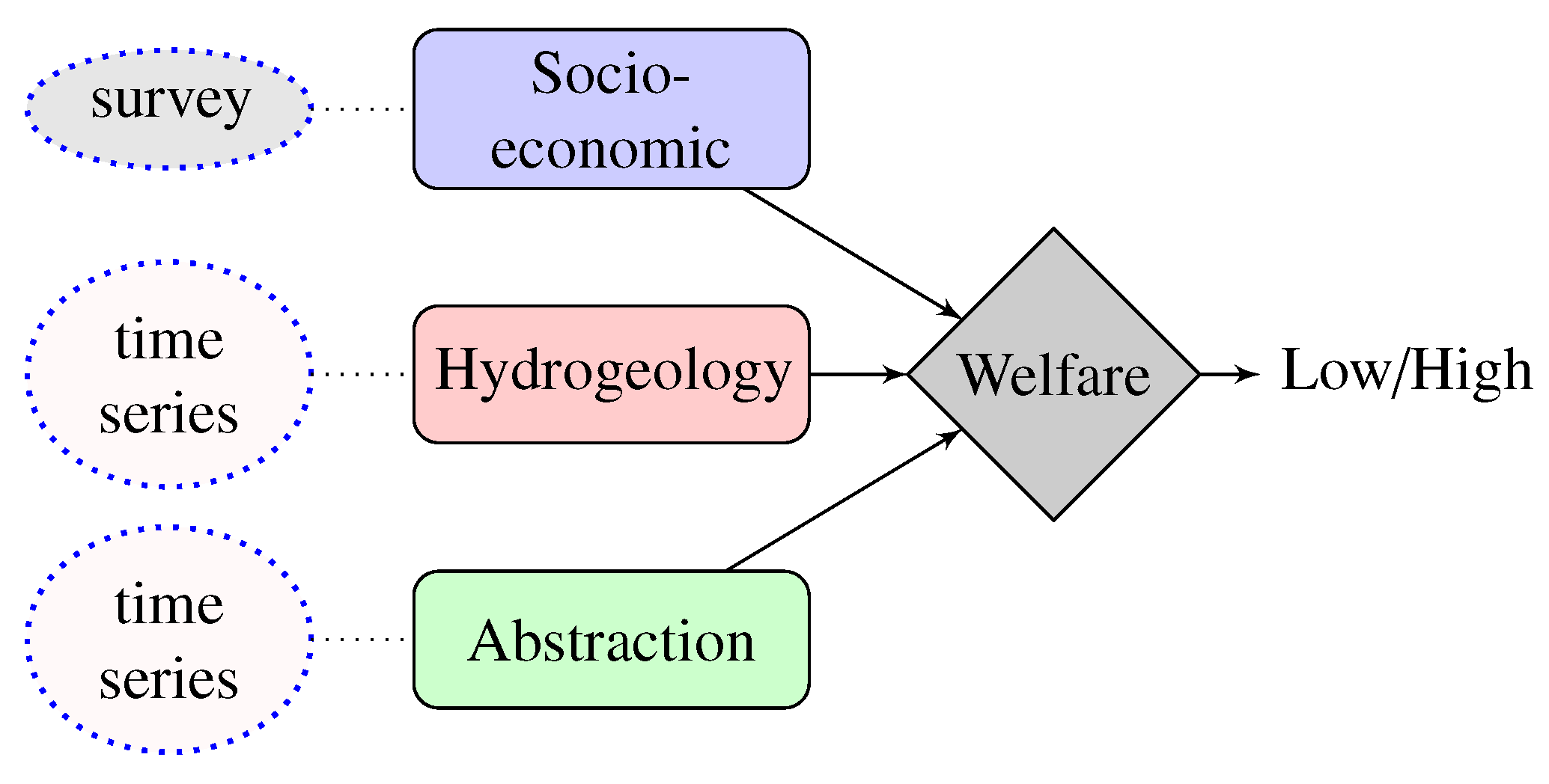
In this section, we discuss the proposed methods to predict the welfare status of a household. The block diagram depicting the objective of the proposed framework is described in Figure 2. We predict the welfare status of a household based on three different modalities of data: (a) socio-economic survey data, (b) groundwater levels, and (c) handpump abstraction data.

The different modalities of data survey, groundwater levels and abstraction are represented as ${\mathbf{x}}_s\in {\mathbb{R}}^{m_1},{\mathbf{x}}_h\in {\mathbb{R}}^{m_2}$ and ${\mathbf{x}}_a\in {\mathbb{R}}^{m_3}$ respectively. The abstraction and groundwater levels data are time-series data while the survey data is a fixed set of questions for a particular household.

The problem here is multidimensional, whose inputs are non-Gaussian and may be correlated, with varying degrees of noise and artefacts present in each signal. Therefore, we will model relationships within different modalities of data using a multi-input multi-output neural network, a framework for modeling multi-modal data. The final output of the model is a set of varying probabilistic indices modeling the welfare that incorporate both dynamical trend information and subtle correlations that may exist between the multidimensional data. There are a total of four welfare indices at the output of the model, one for each modality of the data, and one final welfare for the joint model.

The multi-input multi-output framework of the neural network allows the uncertainty in the data to be modeled explicitly, allowing the output of the model to cope with signals that are (a) sampled at different times, and (b) corrupted by varying degrees of artefact and noise. In addition, the proposed method is non-parametric, and therefore can scale to the modeling of very large quantities of big data in a principled manner, where model structure is learned directly from the data, rather than by imposing strong probabilistic modeling assumptions. Furthermore, the welfare status estimated at the output of the model allow the relevant institutions and stakeholders to explore the status and risks being faced by different households and act accordingly.

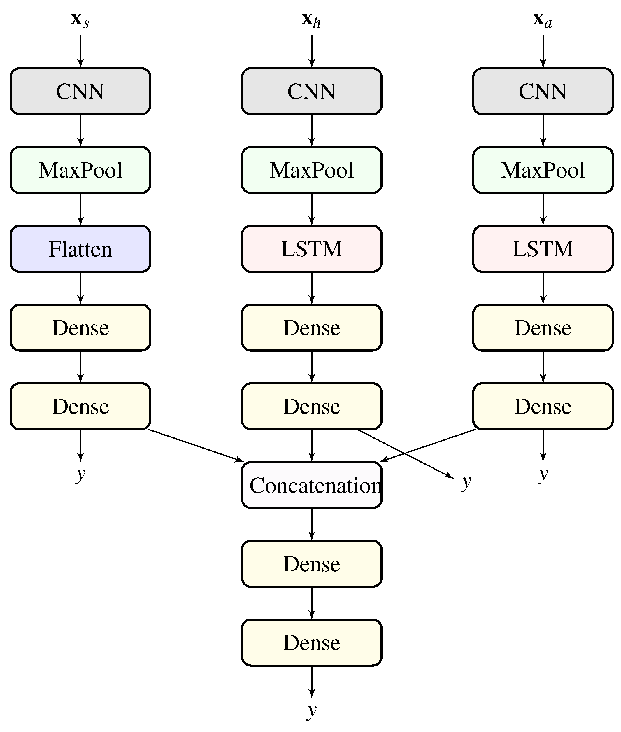
The block diagram of the proposed framework is shown in Figure 3. This framework consists of three smaller sub-networks, one for each individual data modality. The different modalities (${\mathbf{x}}_s,{\mathbf{x}}_h,{\mathbf{x}}_a$) of the data are the inputs to each of the smaller sub-networks, and the output of all networks correspond to welfare label (y). The embeddings from the penultimate layers of each of the smaller neural network are concatenated and are fed to a series of fully connected layers, with welfare label (y) as the final output. The resulting multi-input multi-output neural network architecture is jointly trained.

The sub-network for the survey data consists of a one-dimensional CNN (1D-CNN) followed by fully connected layers. A CNN is a sequence of layers, where each layer takes a multidimensional array as input and gives a multidimensional as output. Mathematically, at each of the layer ${\mathbf{y}}_s=c\left({\mathbf{x}}_s\right)$, where ${\mathbf{x}}_s$ and ${\mathbf{y}}_s$ are the input and output arrays respectively and c is a local function, consisting of translation invariant operators and thus can be considered as a filter. The convolution operation is generally followed by a pooling step which is computed over the input array in small sliding windows. Among different types of pooling functions, e.g., averaging and sum, maxpooling is the one most commonly used. This CNN module is followed by a maxpooling operator. Furthermore, a flattening layer flattens the data before it is fed to a multi-layer FF network with two fully connected layers. The multi-layer FF network consist of a cascade of perceptron layers. The individual perceptron layer is defined as:

$${\mathbf{y}}_p=\sigma (\mathbf{W}{\mathbf{y}}_s+\mathbf{b}),$$

(1)

where $\mathbf{W}$ is the weight vector matrix, ${\mathbf{y}}_s$ is the input vector, $\mathbf{b}$ is the bias, and $\sigma$ is the activation function. The last fully connected layer is connected to a SoftMax layer with two classes.

Since groundwater levels data is a time-series, Long Short-Term Memory networks (LSTM), a type of RNN suitable for time-series data, is used to model the data. The sub-network for groundwater levels data consists of a 1D-CNN followed by a LSTM layer further connected to a series of fully connected layers. 1D-CNN in this sub-network can be considered to be an inbuilt feature extractor. LSTM can learn long term dependencies in the time-series data and have the form of a chain of repeating cells. Each LSTM cell has a forget gate $f_t$, input gate $i_t$ and cell state $C_t$. The forget gate decides which information is discarded from the previous cell state. On the contrary, the input gate, based on the current input decides which information is stored in the current cell state. Based on the previous two steps, the cell state stores which information to forget and store. For a given time series ${\mathbf{x}}_h=\{x_1,\cdots ,x_t,\cdots ,x_{m_2}\}$, as input, a LSTM employs following steps:

$$\begin{array}{cc}\hfill {\mathbf{f}}_t& ={\sigma }_1({\mathbf{W}}_f{\mathbf{h}}_{t-1}+{\mathbf{W}}_f{\mathbf{x}}_t+{\mathbf{b}}_f)\hfill \\ \hfill {\mathbf{i}}_t& ={\sigma }_1({\mathbf{W}}_i{\mathbf{h}}_{t-1}+{\mathbf{W}}_i{\mathbf{x}}_t+{\mathbf{b}}_i)\hfill \\ \hfill {\mathbf{C}}_t& ={\mathbf{f}}_t\times {\mathbf{C}}_{t-1}+{\mathbf{i}}_t\times {\sigma }_2({\mathbf{W}}_c{\mathbf{h}}_{t-1}+{\mathbf{W}}_c{\mathbf{x}}_t+{\mathbf{b}}_c).\hfill \end{array}$$

(2)

Finally, an output gate modulated by the cell state computes the hidden layer state as:

$${\mathbf{h}}_t={\sigma }_1({\mathbf{W}}_h{\mathbf{h}}_{t-1}+{\mathbf{W}}_h{\mathbf{x}}_t+{\mathbf{b}}_h)\times {\sigma }_2\left({\mathbf{C}}_t\right),$$

(3)

where ${\sigma }_1$ and ${\sigma }_2$ are two activation functions, sigmoid and tanh, respectively. ${\mathbf{W}}_{*}$ and ${\mathbf{b}}_{*}$ indicates the weight matrices and the biases, respectively, and t represents the time index. Here * can be $f,i$ and c, representing the parameters for forget gate, input gate and the cell state, respectively.

Since abstraction data is also a time-series, a LSTM sub-network, similar to the one used for groundwater levels, is employed for modeling the abstraction data. The outputs of the penultimate layers for survey, groundwater levels, and abstraction data, represented by ${\mathbf{d}}_s,{\mathbf{d}}_h$, and ${\mathbf{d}}_a$ respectively, are concatenated, $\mathbf{d}=[{\mathbf{d}}_s,{\mathbf{d}}_h,{\mathbf{d}}_a]$, and fed to a FF network with two layers. For reference, this entire network is also compared to smaller sub-networks that consider individual datasets separately for welfare prediction, here each individual dataset is modeled by the corresponding sub-network described above.

3. Experimental Setup

This section starts with the detailed description of the dataset along with the problem formulation. Furthermore, we describe the details of various hyper-parameters of the proposed classifiers employed in this work.

3.1. Dataset Description

The dataset consists of three modalities: socio-economic survey, abstraction, and groundwater levels. There are challenges to employ these datasets simultaneously in a single model. A detailed description of these datasets and their limitations are as follows.

3.1.1. Socio-Economic Survey Data

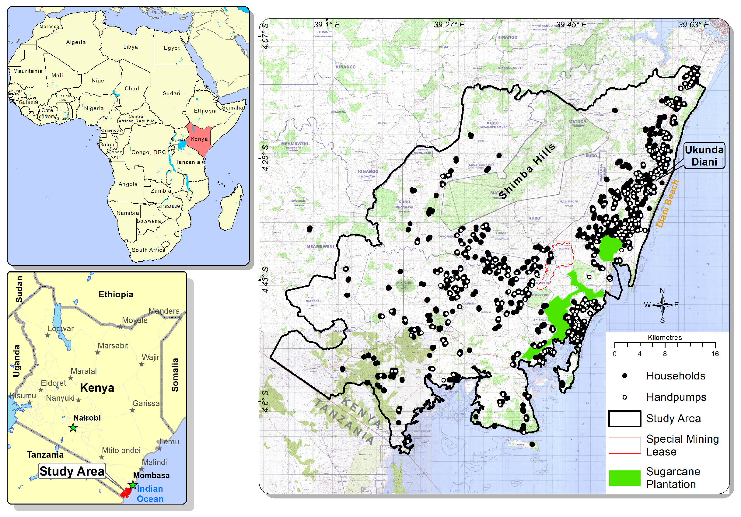
The socio-economic data was collected as part of three rounds of longitudinal household surveys between 2013 and 2016 with respect to a sample of 532 handpump locations [29,30]. The data collected at each of the longitudinal survey is considered to be data belonging to one year. For each handpump location, an average of six households are randomly selected, generating a sample of 3,500 households. The survey captured information related to household demographics, welfare indicators and household assets, health, drinking water supplies, waterpoint management, and subjective welfare assessments. From these data a set of 29 indicators (${\mathbf{x}}_{s_t}\in {\mathbb{R}}^n$) are used to derive an asset-based multidimensional welfare index with weights defined by principal component analysis (PCA) approach [29,31,32]. This approach differs from income or expenditure measures of poverty where a household would be classified based on one dimension of well-being with a poverty line cut-off which in some cases may be subjectively pre-selected. Welfare is a more inclusive concept acknowledging multiple dimensions such as education, health, assets and other salient indicators.

For this study, the resulting welfare index, normalized between 0 and 1, is used to divide the population into two halves—we consider households with welfare index less than 0.5 to be low-welfare, and the rest high-welfare. These low-welfare vs. high-welfare households are considered to be ground truth labels. A different subset of five questions (${\mathbf{x}}_s$) assumed to represent the how well off a household is, are used as inputs to train the models. Based on wider literature [29], we select five indicators at the household level: (i) gender of head, (ii) dependency ratio (children over 15 years/total adults), (iii) improved structure (walls are rendered), (iv) own cattle or oxen, (v) subjective perception of being better off. These five questions are different from the 29 questions used to generate the labels to avoid learning a trivial mapping function. The key motivation behind using fewer survey questions to model welfare status is to ensure the proposed framework can be employed in resource-constrained settings, where performing periodic comprehensive surveys may be unfeasible. A potential solution may be asking a small subset of questions by mobile phone survey rather face-to-face interviews.

3.1.2. Groundwater Level Data

A groundwater flow model was developed to characterize the aquifer system of southern coastal Kenya. Following the development of a conceptual model [18] a numerical model was constructed using Modflow-2005, simulating the period 2010 to 2017 and eight future model scenarios [24]. As outputs of this model, estimated water levels of the aquifer system for the study area are available at 10-day intervals during 2010–2016. For this study, we assume a time-series of past $m_2$ intervals of water levels at a household’s location to represent the state of drinking water supply for that household (${\mathbf{x}}_h$). Since we observed that for most of the temporal windows, the change in water levels was very subtle, we use area under the curve as opposed to the raw values. This representation of available water supply has its limitations. The water levels alone do not characterize household water availability, accessibility, and reliability, which are all key factors as defined under sustainable development goals [33]. A more nuanced approach would be to include additional data such as the distance to the nearest operational handpump, cost (if any) of accessing the pump, quality of water, etc. As one of the aims is to investigate whether a limited data set can provide useful extra information about household welfare, we limit ourselves to using the modeled water levels to represent the state of the water supply.

3.1.3. Abstraction Data

GSM-enabled transmitters were installed on a sample of 300 operational community handpumps to generate daily pump usage data [19,34]. For this study, the daily data over 2013-2016 is converted into average weekly data. We assume a time-series of past $m_3$ weeks of average weekly abstraction (${\mathbf{x}}_a$) represents the water demand of households using that pump. We note there are limitations to this assumption: (1) handpumps abstraction data alone is not representative of the water demand because people also use other sources of water (e.g., river, open wells, rain water, etc.), (2) the data represents average abstraction of the pump which cannot be disaggregated into individual households using the pump, (3) the data cannot be disaggregated into usage by types, i.e., household vs. irrigation vs. livestock activities, and (4) the data has missing values due to many reasons, e.g., pump malfunction, pump not being used temporarily due to availability of other resources (e.g., rainfall, school closures). For this data, it is difficult to overcome the first three limitations but regarding missing data, we propose some potential approaches in Section 4.2 to alleviate the problem.

Thus, each household specific example is represented by three types of data modalities—${\mathbf{x}}_s$, ${\mathbf{x}}_a$, and ${\mathbf{x}}_h$, which are the features, along with corresponding welfare label y. A collection of these examples is used to train the machine learning approaches described in Section 2. We also use different combinations of these feature to analyze their mutual benefits.

3.2. Model Parameters

In this section, we discuss the experimental setup along with the details of various parameters used in the experiments. The 1D-CNN layers use 16 filter banks with kernel size/stride of 3/1 and all the LSTM layers have 32 nodes. The maxpooling operator is employed with 3 steps and the last two dense layers in each sub-network have 8 and 16 nodes. The concatenated representation is followed by two dense layers with 32 and 16 nodes, respectively. The last fully connected layers of each submodel and joint model are connected to a SoftMax layer with two classes.

All of the networks for this paper are trained using Keras [35] with Tensorflow [36] backend. The rmsprop optimizer is used with an initial learning rate of ${10}^{-3}$. All the networks are trained for 100 epochs with a batch size of 32. The loss function used in all the sub-networks and the overall network is binary crossentropy with accuracy as the metric for classification. The overall loss used is weighed by 0.8, 1, 0.5 and 0.5 for the overall network, sub-networks for survey, groundwater levels and abstraction data, respectively. The 1D-CNN layers employ ReLU [1] as activation and sigmoid is used as activation at the last layer of each of the network. The experiments with individual modalities of data employs each of the respective sub-network. The socio-economic survey data used in all the machine learning experiments ${\mathbf{x}}_s$ is a set of five questions ($m_1$ = 5). The data corresponding to past ten time-intervals of groundwater levels data are used as ${\mathbf{x}}_h$ ($m_2$ = 10). Similarly, the data corresponding to the average handpump water level abstraction for past eight weeks is used as ${\mathbf{x}}_a$ ($m_3$ = 8). All the hyper-parameters and dimensionality of representations corresponding to both the ${\mathbf{x}}_h$ and ${\mathbf{x}}_a$ are obtained empirically.

In case of abstraction data, ${\mathbf{x}}_a$, when the data is missing for two consecutive days, we use the average abstraction level for the following and previous 4 days. If the data for a particular handpump corresponding to the respective household is unavailable, the data belonging to the nearest handpump is used. However, as we vary the distance to the nearest handpump to a household with available data, the number of households available to model varies.

The data corresponding to both ${\mathbf{x}}_h$ and ${\mathbf{x}}_a$ are normalized. The socio-economic survey data is collected over three periods and attempted to cover the same households over time; however, the households from one period to the other does vary. In this work, for most of the experiments, we consider these households to be independent. In all experiments the distance of handpump used for abstraction data is less than 0.5 km, resulting in 3259 households, unless stated otherwise. The year-wise data split for low-welfare/high-welfare households is year one—583/620, year two—263/524 and year three—350/919. We evaluate the performance using classification accuracy (CA) and area under the receiver operating characteristic curve (AUROC) as metrics.

4. Experimental Observations

This section provides a detailed explanation about various experiments starting with the year-wise cross-validation, where the total data belonging to two years of survey is used to train the model and the data belonging to the third year is used for testing. Furthermore, we evaluate the performance of the proposed model when the data from nearby handpumps is used as abstraction data for the households with missing abstraction data. The performance of the welfare prediction model is analyzed for various sections of the geographical locations of households. Finally, a comparison of the proposed method with the traditional machine learning methods is also provided.

4.1. Year-Wise Cross Validation

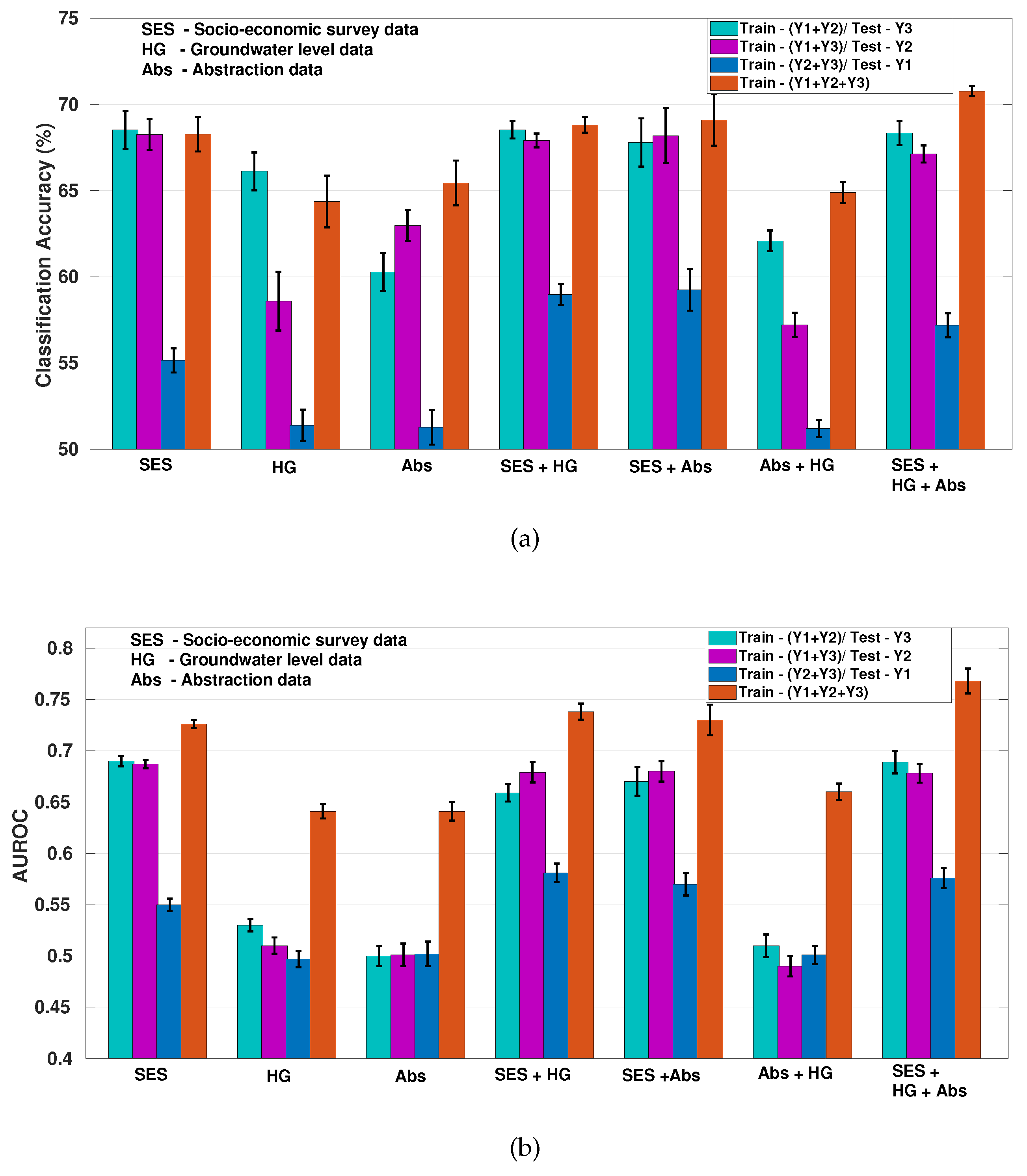
In this experiment we have employed a combination of two different years of survey data (along with other two input modalities) as training data and the third year as testing. In addition, we have also employed each one of the ${\mathbf{x}}_s$, ${\mathbf{x}}_h$ and ${\mathbf{x}}_a$ individually and in tandem with each other for the same task. We have also pooled the survey data belonging to three years together for a three-fold cross-validation. The results for these different experiments are shown in the form of CA and AUROC (with 95% confidence interval (CI)) in Figure 4a,b respectively.

It can be observed that there is complementary information in different modalities as evident from the results for all the data (brown bars). These results are consistent when year one and year two data is used for training and year three is used for testing, except a slight peak in the results for socio-economic survey and groundwater levels data as input.

The results when years two and three are used for training are different from other results, especially for the case of groundwater levels and abstraction data. One possible reason for this could be the temporal information present in the abstraction and groundwater levels data. The testing data here belongs to the previous year as compared to the training data, maybe the lag in temporal dimension of groundwater levels and abstraction data results in bad performance. This observation above is further strengthened by viewing the results using only the socio-economic survey data, here the CI is much smaller for the year-fold validation as opposed to the CI for groundwater levels, abstraction or groundwater levels and abstraction data.

4.2. Missing Abstraction Data

To deal with missing values in abstraction data, whenever household specific handpump abstraction data is unavailable, for that household, we consider data from the next closest representative handpump with available data. The AUROC results with 95% CI for a three-fold stratified cross-validation of the total pooled dataset as we vary the distance (in kms) of closest handpump are shown in

Table 1. AUROC with 95% CI for different modalities data as input with the varying distance for the handpump data used for the abstraction data. #HH here represent the number of households. SES, Abs and HG represents socio-economic survey, abstraction and groundwater levels data.

		AUROC
Distance	#HH	SES	HG	Abs	SES + HG	SES + Abs	Abs + HG	SES + HG + Abs
<0.2	2200	0.71 ± 0.009	0.65 ± 0.01	0.66 ± 0.012	0.72 ± 0.007	0.74 ± 0.005	0.67 ± 0.010	0.78 ± 0.014
<0.5	3259	0.72 ± 0.004	0.64 ± 0.007	0.64 ± 0.009	0.73 ± 0.008	0.73 ± 0.015	0.66 ± 0.008	0.77 ± 0.012
<1	3700	0.70 ± 0.007	0.63 ± 0.005	0.66 ± 0.011	0.71 ± 0.010	0.74 ± 0.008	0.67 ± 0.013	0.76 ± 0.009
<2	3700	0.71 ± 0.008	0.66 ± 0.011	0.65 ± 0.010	0.73 ± 0.005	0.73 ± 0.007	0.66 ± 0.007	0.76 ± 0.010
-	4204	0.72 ± 0.010	0.64 ± 0.009	0.66 ± 0.013	0.72 ± 0.009	0.74 ± 0.012	0.67 ± 0.005	0.77 ± 0.015

. We observe that the proposed method performs almost similar in all the cases when this distance is varied. One of the possible reasons could be the similarity between the average weekly abstraction data for different handpumps over a region. It may be the case that the model is able to capture the region-based variations which are not much different. However, in all these cases the use of abstraction and the groundwater levels data improves the performance. This further supports our claim that there is complementary information in the abstraction and groundwater levels data which can assist in welfare prediction for a household.

4.3. Location Based Performance

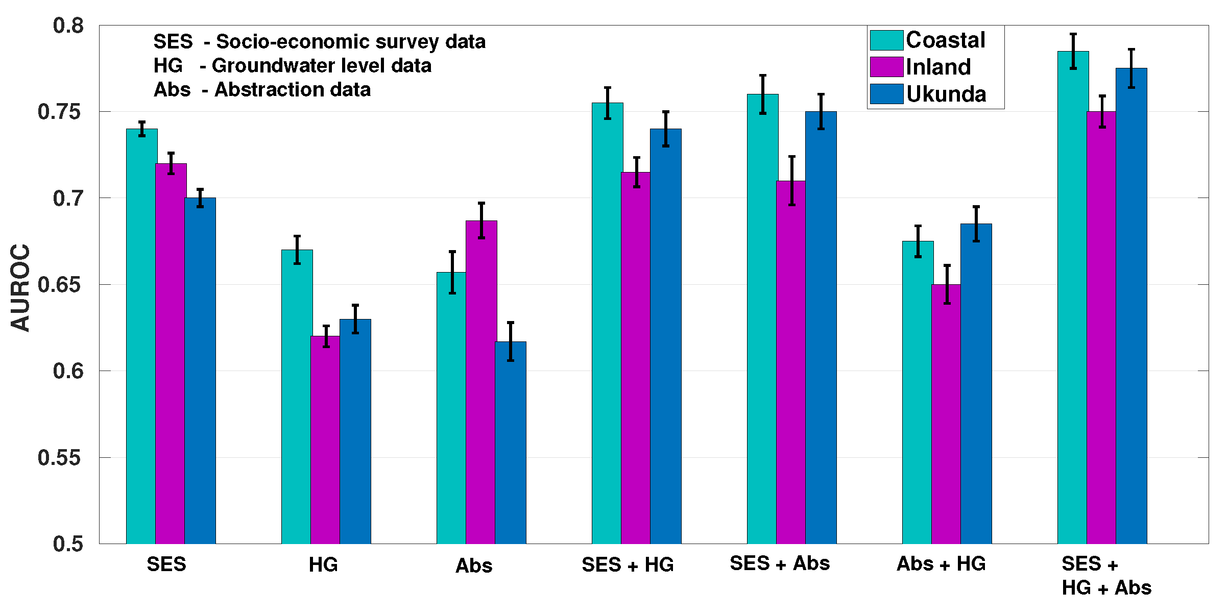
In an attempt to assess the differential value of the proposed model with respect to geographical location of the study area, we disaggregate the model outputs by specific zones. Although there are no physical boundaries separating these zones, the study area consists of three distinct zones based on geographical characteristics livelihood activities—Ukunda (urban, tourism, some access to piped water), coastal (rural, fishing, water drawn from shallow wells in a karstic coral aquifer), and inland (rural, mining, and commercial irrigation, water from boreholes a sandstone aquifer). The total number of households sampled in coastal, inland and Ukunda regions are 2355, 1361 and 488, respectively. The AUROC (with 95% CI) plots for a three-fold stratified cross-validation, with different modalities of data as input, for different regions are shown in Figure 5.

The benefits gained from the addition of water level and abstraction data to the socio-economic data varies substantially over the three zones. Inland, the addition of the water level and abstraction data raises the mean AUROC by only 3% (this reduces further if considering the 95% CI). Also, compared to the other two zones the predictive power of the water level data and abstraction data are very different, with the abstraction data being more useful, although still less useful than the socio-economic data. In contrast, the addition of the water level and abstraction data is most beneficial in predicting welfare in the Ukunda region, adding a further 8% to the AUROC.

Given their geography, the inland communities will arguably be more affected by their environment, in particular the state of the aquifer than those in other area. Groundwater is not as easily accessible as it is at the coast, with boreholes drawing water from 30 m to 40 m, as opposed to shallow dug wells less than 10 m deep. Inland households must be more resilient to changes in groundwater levels as if they are not, the consequences will be more deleterious. Similarly, handpump density is much lower making the distance to one’s second water sources much greater than at the coast. Thus, the other measures of welfare may have groundwater levels and abstraction effects built into them. In addition, Figure 5 shows that for the inland household abstraction alone is a better predictor of welfare than in other areas. Related research in the same study area [27] showed that handpump use is closely linked to rainfall patterns and that household in this area are more likely to harvest rainwater. This is consistent with there being a closer correlation between handpump abstraction and other welfare-related factors implied by the higher ‘abstraction only’ AUROC in this area relative to the coastal and Ukunda regions. This deserves further investigation beyond the scope of this paper and these datasets.

4.4. Comparison with Other Techniques

The proposed method is also compared with the standard machine learning algorithms as shown in

Table 2. Comparison of the proposed method with the standard machine learning classifiers for the data in terms of CA (%), AUROC, Precision and Recall. The data used in this experiment have all the modalities as input.

	KNN	SVM	DT	RF	MLP	1D-CNN	Proposed
CA (%)	65.18 ± 1.3	71.63 ± 0.9	68.13 ± 0.7	69.18 ± 1.1	67.04 ± 0.93	70.19 ± 0.87	70.78 ± 0.30
AUROC	0.57 ± 0.02	0.59 ± 0.004	0.64 ± 0.011	0.67 ± 0.007	0.73 ± 0.009	0.74 ± 0.011	0.77 ± 0.012
Precision	0.58 ± 0.04	0.58 ± 0.006	0.65 ± 0.009	0.67 ± 0.005	0.71 ± 0.010	0.72 ± 0.008	0.79 ± 0.010
Recall	0.57 ± 0.03	0.59 ± 0.004	0.64 ± 0.007	0.69 ± 0.009	0.74 ± 0.007	0.73 ± 0.007	0.77 ± 0.009

. The metrics used for comparison are CA, AUROC, precision and recall, the results are shown with 95% CI for three-fold stratified cross-validation for all the pooled data. The input data used for this experiment consists of all three modalities of data. The methods used for comparison are K-nearest neighbors (KNN), support vector machine (SVM), decision trees (DT), and random forest (RF) [2,37]: the number of nearest neighbors chosen for KNN classifier are five; SVM are implemented with a radial basis function (RBF) kernel; the criterion used for the DT is gini impurity with ten minimum samples required for split. The RF classifier fits a number of DT classifiers on various sub-samples of the data and employs averaging to improve the performance.

In addition, we have also employed a standard machine learning classifiers, a multi-layer perceptron (MLP) and 1D-CNN-based deep neural network [1]. The MLP employed here is a FF network with four layers with 32, 16, 64 and 32 nodes with a dropout of 0.2 after each layer. The 1D-CNN network consists of a 1D-CNN followed by a FF network, the CNN layer have 16 filterbanks with kernel size and stride of 3 and 1, respectively. This is followed by three FF layers with 32, 16 and 32 nodes, a dropout of 0.2 is used here as well. All other hyper-parameters in these networks are similar to the proposed network. It can be observed that the proposed multi-input multi-output neural network outperform the existing machine learning models for our task. It can be observed that the proposed multi-input multi-output neural network is not only outperforming the traditional machine learning methods, but is also better than a standard MLP and CNN-based classifier. In case of AUROC, the proposed method results in a gain of 4.05% as opposed to the 1D-CNN-based model, which is the best performing model among all other models. There could be two possible reasons for better performance: (a) efficient modeling of time-series data in abstraction and groundwater level data using LSTM, and (b) knowledge transfer in the multi-input multi-output deep learning method employed. The proposed model is jointly trained, and hence different modalities will have more interactions during the error backpropagation (in training). Thus, the network may learn hidden representations which contain knowledge that is trained and used by different modalities of data. The hidden representations trained this way will be better than the one estimated in a single model.

5. Conclusions and Discussion

In this work, we have demonstrated that a small set of survey questions along with groundwater level and handpump abstraction data can be used to predict the welfare status of households. Groundwater level and abstraction data alone perform worse as a predictor of welfare, as was expected; however, abstraction is slightly more predictive than water level. Combining abstraction and groundwater levels with survey data improves the performance; however, this gain varies across different regions within the study area, in some areas adding little value. When used in isolation abstraction and groundwater levels may not be what one would choose as an indicator of welfare around which one might design programs and interventions. But the fact that they do have some predictive power demonstrates that, in this locale at least, the water resources and water abstracted are linked to household welfare.

Comprehensive household surveys, rightly so, remain popular tools for determining welfare. Despite providing vital information, a major challenge with their use is that they are time-consuming and resource-intensive. The proposed framework provides an alternative solution by using a relatively small set of survey questions along with complementary available datasets, e.g., from groundwater levels and handpump abstraction data, to estimate the welfare status of households.

We have shown here that, in conjunction with small set of socio-economic survey data, water level and abstraction data provide useful additional information to characterize the welfare status of households. This method may be useful to policymakers, especially when they must allocate scarce resources efficiently, with only limited data available to inform their decision making. In future, other modalities of readily available data can also be employed in this type of a model to further improve the performance.

We draw three main lessons from this work from modeling multiple streams of data in one of the most intensively researched, rural study sites in Africa. First, the data requirements for machine learning methods are large. The groundwater level, daily abstraction data from handpumps and three panels of a large, longitudinal survey do not elicit clear and compelling results despite an extensive portfolio of modeling treatments. Given advances in remote sensing technologies, data resolution and multiple data sources, there is a strong case to conduct further work to validate the findings presented here. The replicability of the field methods applied in this study are unlikely to be available in all but the most strategic locations in Africa.

Second, the modeling has revealed a muted but intriguing signal that welfare may be associated with the patterns of daily water abstraction from handpumps. This partly reflects the notion of accidental infrastructure where one data stream may contain artefacts of useful information for other purposes. There is insufficient evidence to claim any predictive power from handpumps as sentinels of welfare, particularly given the multidimensional nature of welfare and poverty. However, it reflects the spill-over effects of collating data in structured and continuous fashion at the interface between biophysical and social systems.

Third, the interactions between groundwater and human welfare are dynamic and masked by biophysical processes and social practices. Though we have evidence that drinking water is one of four, dominant welfare priorities in the study area [38], it is ranked below education, energy or sanitation. As we have noted, there are a range of confounding factors which reject any simple causal relationship to hold between groundwater and welfare. The implication that abstraction from rural handpumps is a proxy for the risk status of households may be substantiated by wider work in this study area where it has been shown that dependency and use of handpumps is seasonal and that the majority of the population depends on groundwater in times of dry spells [29,39]. The extent to which handpump abstraction is a proxy for risk is therefore plausible and worthy of further exploration to examine unknown aspects of distributional inequalities for different social groups access to and use of handpumps.

In conclusion, we would identify three major limitations to this work which merit consideration in future applications. First, the proposed method involved combining different modalities of data to improve the performance, but it is challenging to combine the varying level of noise and conflicts between modalities. One of the biggest challenges here is learning how to represent and summarize multi-modal data such that the complementary information is emphasized and redundancy is reduced. The multi-modal data is heterogeneous, and the relationship between modalities is open-ended or subjective, which makes it challenging to translate (map) data from one modality to another. Other challenges here include identifying the direct relations between elements and joining information from two or more different modalities. Second, we would also like to point out that there are limitations with the use of PCA-based method employed to generate ground truth labels for our task. Third, our welfare is framed here by five socio-economic variables chosen based on judgement and published literature. There are grounds to test and refine other risk proxies derived from both social and biophysical sources of information in future work.