Anomaly Detection System for Water Networks in Northern Ethiopia Using Bayesian Inference

Abstract

For billions of people living in remote and rural communities in the developing countries, small water systems are the only source of clean drinking water. Due to the rural nature of such water systems, site visits may occur infrequently. This means broken water systems can remain in a malfunctioning state for months, forcing communities to return to drinking unsafe water. In this work, we present a novel two-level anomaly detection system aimed to detect malfunctioning remote sensored water hand-pumps, allowing for a proactive approach to pump maintenance. To detect anomalies, we need a model of normal water usage behavior first. We train a multilevel probabilistic model of normal usage using approximate variational Bayesian inference to obtain a conditional probability distribution over the hourly water usage data. We then use this conditional distribution to construct a level-1 scoring function for each hourly water observation and a level-2 scoring function for each pump. Probabilistic models and Bayesian inference collectively were chosen for their ability to capture the high temporal variability in the water usage data at the individual pump level as well as their ability to estimate interpretable model parameters. Experimental results in this work have demonstrated that the pump scoring function is able to detect malfunctioning sensors as well as a change in water usage behavior allowing for a more responsive and proactive pump system maintenance.

1. Introduction

Water-related diseases are responsible for 80% of the death and illness in the developing world [1]. For an estimated 2.9 billion people living in remote, rural communities in developing countries, small water systems are the only source of clean and safe drinking water [2]. In rural sub-Saharan Africa, the majority of those who enjoy access to an improved source of water, mostly rely on boreholes with hand-pumps [3]. Despite the billions of dollars of investments in the development of such remote water systems, providing water service to people lacking access to drinking water facilities and ensuring the service is reliable and sustainable remains a significant challenge [4,5]. In fact, the number of rural sub-Saharan Africans without access to safe drinking water has risen from 240 million in 1990 to 275 million in 2011 [4]. Historically, the only way for governments and non-government organizations to monitor rural water systems has been to visit them. But reaching these locations takes time, human resources, and money. Given this reality, site visits occur infrequently, meaning broken water systems can stay broken for months. Estimates by Foster et al. [6] show that 33% of water points in Ethiopia are non-functional, and many of these water points will never be repaired. When these water systems go down, communities have no choice but to go back to drinking dirty water leading to significant adverse health implications, and a slow down in other human development gains [7,8]

As part of charity: water’s—a non-profit organization [9]—efforts to improve the sustainability of water projects, a special program to develop a remote sensor was launched in 2012, with the support of a grant from Google [10]. The goal was to harness the power of what’s being called the Fourth Industrial Revolution [11] and put IoT (Internet of Things) and cloud computing technology to work for the world’s poorest people. charity: water, along with other technology partners, developed a remote sensor device to monitor performance and functionality of clean water projects located in remote areas of the developing world. The sensor transmits real-time water flow data to the cloud, so if a pump breaks down, mechanics can be dispatched to restore clean water as quickly as possible. Collecting and harnessing such real-time data could significantly improve the sustainability of water services in rural communities [12].

The first round of funding enabled engineers to develop the first iteration of the Afridev hand pump sensor, Afridev-1 [13], which is a sensor built to wrap around the rising main pipe and measure the water level in a central chamber. See Figure 1. Starting in late 2015, the first generation of the water sensor was deployed on 3000 Afridev hand pumps in Northern Ethiopia. Inside each device, a stack of six capacitance sensors measure the physical level of water in the wellhead twice every second, which is then converted to liters per hour flowing through the pump [13]. The data from the sensors installed can be viewed online. We refer the reader to Appendix A for details on how to login and view the data.

The devices deployed in 2015 have collected millions of data points since installation and the purpose of this study was to analyze this data. One immediate goal was to identify anomalies in the data. This is important for two main reasons. First, once anomalous elements are identified in the data, they can be removed resulting in a cleaner dataset to learn better models of normal water usage. This will be important to better understand user water consumption characteristics and identify patterns and seasonality effects. Second, the anomalies themselves can be of interest as they may show rare changes in water consumption behavior or detect faulty sensors early, which will drive better maintenance practices and resource management. Understanding and analyzing water consumption patterns will help drive the next generation sensor design and feedback into rolling out a predictive element to the next generation device.

In this work, we present an anomaly detection approach to the aforementioned water usage data. We first fit a multilevel probabilistic model of normal water usage using approximate variational Bayesian inference to obtain a conditional probability distribution over the hourly data. This will be our model of normal. We then use the conditional distribution—model of normal—to form a scoring function for each water observation and a scoring function for each pump. The pump-level scoring function derived from the Irwin-Hall cumulative distribution function will be used to score each pump from the aggregated observation-level scores produced by the observation-level scoring function. If the pump-level score indicates an anomalous pump, then the observation-level score is used to investigate which specific set of observations contributed to the high pump score. The approach is semi-supervised, meaning that only data representing normal water usage is needed to fit the model. The model is also interpretable. In other words, this is not a black-box model, and the learnt model parameters could potentially uncover insights related to user water usage characteristics and seasonalities present in the data. The anomaly detection system presented in this work is novel in its hierarchical scoring design by which data is scored for anomalies at two levels (individual observation-level and pump-level) using the same model of normal, while preserving the interpretability of the model parameters. To the best of our knowledge, such a hierarchical anomaly detection system has not been developed for water networks. This design enables water network operators to incorporate their knowledge of the state of the pump by resetting the score in the cases when the anomaly detection system triggers a false anomaly (false positive). This will be discussed further in Section 3.3.

The rest of the paper is organized as follows: First, we provide a literature overview of prior work applying anomaly detection methods to water systems, followed by a discussion of the dataset used in our analysis and how it was collected. Second, we present our multilevel probabilistic model of normal water usage and the inference method used to estimate the model parameters. Following that, we present a discussion of our anomaly detection approach using the probabilistic model of normal water usage. The anomaly detection section is broken down into two parts: an observation-level scoring and a pump-level scoring. Both scoring functions will be discussed. Third, we discuss the model results and the performance of the anomaly detection system on the data we have at hand. We finish the paper with the conclusions and future work.

2. Materials and Methods

Anomaly detection is a critical topic in numerous industry sectors addressing issues such as fraud detection, security, safety in process engineering, manufacturing, infrastructure, distribution systems, and predictive maintenance. A significant amount of research on data-driven anomaly detection has been done using statistical modeling and, more recently, machine learning algorithms, cf. Hodge and Austin [14], Rousseeuw and Leroy [15], Barnett and Lewis [16], Hawkins [17], Bakar et al. [18], Chandola et al. [19]. In particular, due to the diverse and complex nature of water distribution systems, various ‘anomalies’ may occur due to fundamentally different underlying causes, e.g., water leakage, pipe blockage, device condition, and energy efficiency are a few examples, cf. Duan and Lee [20], Duan et al. [21], Islam et al. [22]. Conducting anomaly detection along with meaningful root-cause analysis for such systems often times requires an appropriate combination of human domain knowledge, observational data, and accurate modeling techniques. More recently, and due to its flexibility, Bayesian inference has become a powerful and appealing technique which can address many of the aforementioned challenges in water systems, cf. Duan et al. [23], Rougier and Goldstein [24], Wang et al. [25].

More recently machine learning techniques, including supervised learning methods have been applied to detect and predict hand-pump anomalies where human-verified examples of pump failures were used to train the detection model, cf. Wilson et al. [26], Greeff et al. [27]. Additionally, Support Vector Machine and Support Vector Regression were proposed by Mounce et al. [28], Candelieri [29] to detect anomalies in urban water distribution systems. Pertaining to water usage data, Zohrevand et al. [30] propose using a Hidden Markov Model—a generative probabilistic model—as a means to model the normal water usage behavior and further detect anomalies in water supply systems. While the approaches in [28,29,30] work well to detect anomalies in water usage data, our choice of a multi-level probabilistic model (discussed in details in Section 2.2) was mostly driven by our ability to identify interpretable patterns through the learnt model parameters, that could potentially unlock insights into the water usage characteristics and any seasonality patterns that may affect water consumption behavior in the rural communities. See discussions in Section 3.

2.1. Dataset

At the time of this analysis, 2414 water pumps retrofitted with first generation Afridev sensor, Afridev-1 [13] were online in the Tigray, Ethiopia region. Figure 2 shows the location of the remotely monitored pumps used in the analysis. The Afridev-1 is equipped with multiple sensors, including a modem for communication with the cellphone towers, and an array of six capacitance sensors for measuring the physical level of water in the wellhead at a frequency of 2 samples per second. This high resolution data is then aggregated by the on board micro-controller to the total liters count flowing through the pump per hour [13]. See Figure 1 for more details on the Afridev-1 sensor design and where it is installed on the rising main pipe of the pump [31]. This hourly liters count data is then sent over the telco network to the cloud and stored in a Redshift database on cloud platform by Amazon Web Services, a.k.a. AWS. In addition to the timestamped hourly liters, the database also reports some information about the approximate number of users per pump which is set by the installation crew at the time of installation. The number of users reported by the sensor is fixed and only changes when the crew re-estimates the number of pump users. The data used in the study was collected over 5 years from September 2015 to June 2019. Both the hourly time-series data of the water usage (hourly liters) and the number of pump users were used in the model.

2.2. Model of Water Usage

Multilevel modeling is a popular approach for modeling a variety of problems going beyond the classical individual within group applications [32]. Multilevel models are designed to analyze data with variables from different levels, allowing for estimating group effects simultaneously with the effects of group-level predictors. Typically, the data is assumed to have a hierarchical or clustered structure with one response variable measured at the lowest level and some explanatory variables at all existing levels [33].

We construct a multilevel generalized linear model with Negative Binomial family and log link where the hourly water liters count variable—the response variable—is assumed to be drawn from a Negative Binomial distribution, where its mean (i.e., location) parameter is conditioned on other explanatory variables from different levels. The Negative Binomial Distribution was used for the likelihood of the response variable since the liters reported by the sensor is count integer data, and the Negative Binomial Distribution allows us to model both the mean (i.e., location) parameter and the variance as opposed to using Poisson which has only one parameter that controls the mean and the variance together.

Suppose we have P pumps producing a total of N hourly water usage measurements. Each hour a pump records and transmits the count of liters, x, pumped out of the well in the last hour. This will be the response variable. Each water measurement is tagged with a timestamp. Certain properties of the timestamp are extracted as explanatory variables such as hour of day, day of week, and month of the year denoted by $h\in [1,\dots ,24]$, $d\in [1,\dots ,7]$, and $m\in [1,\dots ,12]$ respectively. These variables are used as different groupings with different levels for the response variable, x. In addition, we include an explanatory variable, r, that represents the number of users that regularly use each pump normalized to have zero mean and unit standard deviation. We found that normalizing the number of users variable made the estimation algorithm more stable. The model of the data looks as follows:

$$\begin{array}{cc}\hfill x& \sim \mathrm{NegBinomial}(\mu ,\varphi ),\hfill \end{array}$$

(1)

$$\begin{array}{cc}\hfill \mu & =exp({\alpha }_0+{\alpha }_h+{\alpha }_d+{\alpha }_m+\beta r),\hfill \end{array}$$

(2)

$$\begin{array}{cc}\hfill \varphi & ={\varphi }_h,\hfill \end{array}$$

(3)

$$\begin{array}{cc}\hfill {\alpha }_0,{\alpha }_h,{\alpha }_d,{\alpha }_m& \sim \mathrm{Normal}(0,{\sigma }_{\alpha }),\beta \sim \mathrm{Normal}(0,{\sigma }_{\beta }),\hfill \end{array}$$

(4)

$$\begin{array}{cc}\hfill {\sigma }_{\alpha }& \sim \mathrm{Half}\text{-}\mathrm{normal}\left(2.5\right),{\sigma }_{\beta }\sim \mathrm{Half}\text{-}\mathrm{normal}\left(1.0\right),\hfill \end{array}$$

(5)

$$\begin{array}{cc}\hfill {\varphi }_h& \sim \mathrm{Half}\text{-}\mathrm{cauchy}\left(1.0\right),\hfill \end{array}$$

(6)

where x is the count of liters pumped measured by the sensor at a given hour (i.e., the response variable). $\mu$ is the mean (i.e., location) parameter of the Negative Binomial distribution, such that $E\left[x\right]=\mu$. ${\varphi }_h$ is the over-dispersion parameter of the Negative Binomial distribution, such that $Var\left[x\right]=\mu +\frac{{\mu }^2}{\varphi }$. The variance parameter ${\varphi }_h$ carries a subscript h for the hour of day group which indicates that the variance parameters will vary across the hours of the day. The log of the mean $\mu$ is a linear function of the explanatory variables, such that the $E\left[x\right]=\mu =exp({\alpha }_0+{\alpha }_h+{\alpha }_d+{\alpha }_m+\beta r)$ and $Var\left[x\right]=\mu +\frac{{\mu }^2}{\varphi }$. ${\alpha }_h$ is the hour of day intercept parameter set, which carries a subscript h∈ [1, …, 24] for the hour of day to allow the mean to also vary across the hours of the day. ${\alpha }_d$ is the day of week intercept parameter set, where d∈ [1, …, 7], ${\alpha }_m$ is the month of year intercept parameter set, where m∈ [1, …, 12]. $\beta$ is the slope parameter associated with the number of users r of a given pump. We only estimate one $\beta$ parameter for the entire population. The Prior used on all intercept parameters ${\alpha }_0$, ${\alpha }_h$, ${\alpha }_d$, and ${\alpha }_m$ is $\mathrm{Normal}(0,{\sigma }_{\alpha })$ where ${\sigma }_{\alpha }\sim \mathrm{Half}\text{-}\mathrm{normal}\left(2.5\right)$. Prior on $\beta$ is $\mathrm{Normal}(0,{\sigma }_{\beta })$ where ${\sigma }_{\beta }\sim \mathrm{Half}\text{-}\mathrm{normal}\left(1.0\right)$, and the Prior on ${\varphi }_h$ is $\mathrm{Half}\text{-}\mathrm{cauchy}\left(1.0\right)$. The model is also represented as a probabilistic graphical model in Figure 3.

We chose weakly informative priors for ${\sigma }_{\alpha }$, ${\sigma }_{\beta }$, and ${\varphi }_h$. The specific choice of the hyperpriors ${\sigma }_{\alpha }$ and ${\sigma }_{\beta }$ was a model design choice. Note that we found no noticeable difference in the estimates for larger values of the variance of the hyperpriors ${\sigma }_{\alpha }$ and ${\sigma }_{\beta }$.

2.3. Inference and Parameter Estimation

We have described the motivation behind the model and illustrated its conceptual usage for understanding water usage and modeling normal behavior. In this section, we turn our attention to procedures for inference and parameter estimation for the model described in Equations (1)–(6).

Bayesian inference is a powerful framework for analyzing data using probability models. First, we formulate a model based on our assumptions of the hidden structures present in the data, assuming that the complex data observed exhibits simpler unobserved patterns. Then, we use inference algorithms to uncover the patterns that are manifested in the data, by approximating the posterior—a conditional distribution of the hidden variables given the data. Finally, we use the posterior distribution to perform the task we have at hand, whether it is forming predictions or simply exploring the data and making inferences. For many machine learning models, the posterior is often difficult to compute, therefore, we resort to approximations.

At the core of Bayesian learning is a conceptually simple principle. Suppose our observed water usage data is X and the explanatory variables ($h,d,m,r$) are represented by W. Suppose also that our model parameters are represented by $\theta =({\alpha }_0,{\alpha }_h,{\alpha }_d,{\alpha }_m,\beta ,{\varphi }_h,{\sigma }_{\alpha },{\sigma }_{\beta })$. The principle tells us how to update our prior belief, $p\left(\theta \right|W)$, about our model parameters $\theta$, using the observed data X and explanatory variables W to obtain a posterior distribution $p\left(\theta \right|X,W)$ over all possible parameter values. This is the famous Bayes’s rule:

$$p\left(\theta \right|X,W)=\frac{p\left(X\right|\theta ,W\left)p\right(\theta \left|W\right)}{p\left(X\right|W)},$$

(7)

where the denominator in Equation (7), $p\left(X\right|W)$, given by

$$p\left(X\right|W)={\int }_{\theta }p\left(X\right|\theta ,W)p\left(\theta \right|W)d\theta ,$$

(8)

is the marginal likelihood which normalizes the posterior distribution such that it integrates to unity. It should be noted that, the integral in Equation (8) is often intractable. In addition, we are often interested in the posterior distribution of a single parameter or a subset of the parameters rather than this joint posterior. Obtaining these marginal distributions also requires computing large integrals that are intractable.

Variational Inference (VI) approximates the posterior distribution with a simpler density [34,35,36]. We search over a family of simple densities and find the member closest to the posterior. This turns approximate inference into an optimization problem. VI has had a tremendous impact on machine learning. It is typically faster than Markov Chain Monte Carlo (MCMC) sampling and has recently scaled up to massive data in Blei et al. [36], Hoffman et al. [37]. Unfortunately, VI algorithms are difficult to derive and require deep expert knowledge. Therefore, we resort to Automatic Differentiation Variational Inference (ADVI) to fit the model to the large dataset at hand.

ADVI is an automatic yet scalable technique to approximate Bayesian inference [38]. The user only provides a dataset and a Bayesian model just like the model described in Equations (1)–(6). The algorithm makes no conjugacy assumptions, and supports a broad class of differentiable models. ADVI follows this high level procedure. First the space of the latent variables (model parameters of interest $\theta$) is transformed to the real coordinate space such that $\mathsf{\Psi }:\mathrm{supp}\left(p\left(\theta \right)\right)\stackrel{}{\to }{\mathbb{R}}^K$, where K is the dimension of $\theta$. Then a Gaussian distribution is posited on the transformed parameters as their variational distribution $\mathcal{N}(\mathsf{\Psi }\left(\theta \right);{\mu }_k^{\mathsf{\Psi }},{\sigma }_k^{\mathsf{\Psi }})$ parameterized by means ${\mu }_k^{\mathsf{\Psi }}$ and the variances ${\sigma }_k^{\mathsf{\Psi }}$ of each Gaussian $k=[1,\dots ,K]$. Finally, as a proxy of minimizing the Kullback-Leibler divergence between the variational distribution and the posterior distribution, we maximize the Evidence Lower Bound (ELBO) using stochastic gradient ascent (the adaGrad variant). Once the optimization converge, the Gaussian variational distribution is then transformed back to the original latent variable space to obtain the non-Gaussian posterior approximation.

ADVI blends automatic differentiation with stochastic optimization to approximate the posterior with attractive convergence properties and speed. For instance, ADVI has complexity $\mathcal{O}\left(2LMK\right)$ per iteration where M is the number of Monte Carlo (MC) samples, L is the number of observations, and K is the dimension of model parameters. Detailed discussion on ADVI and its convergence properties can be found in [38,39,40]. Note that the processing time to approximate the posterior for the parameters reported in this work was 17.8 seconds per 1000 iterations on a 3.1 GHz Intel i5 laptop with 8 GB RAM.

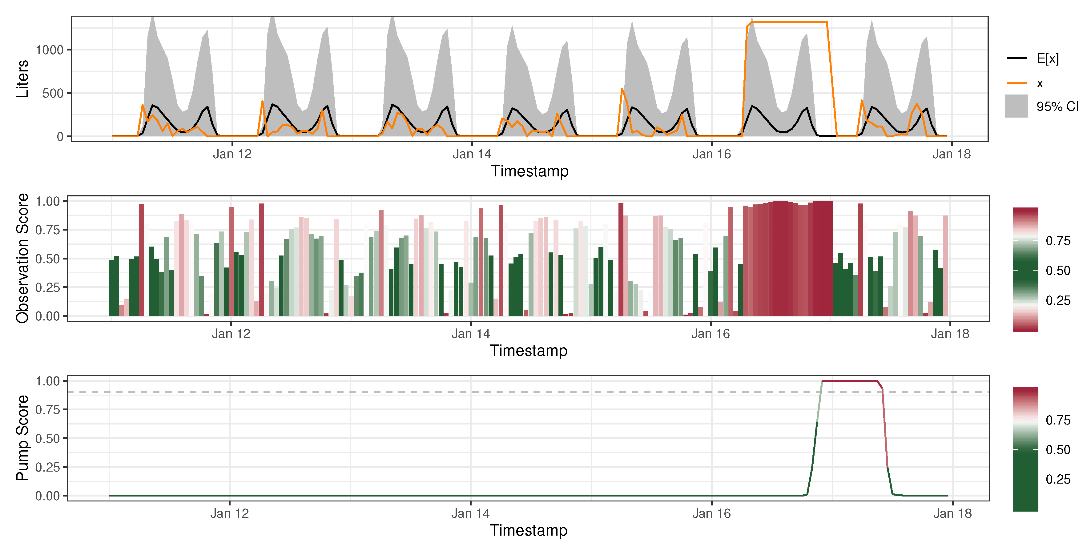
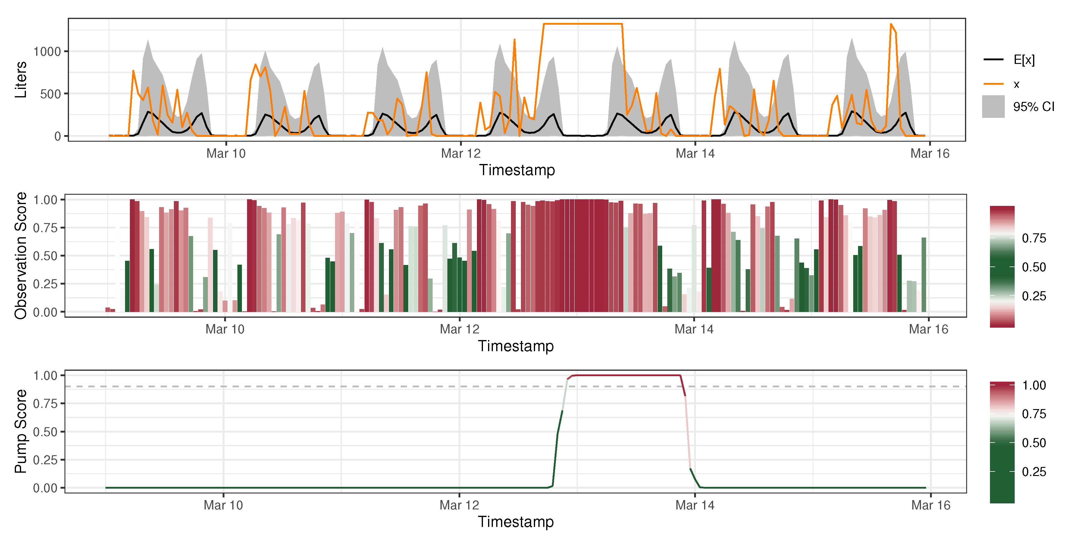
2.4. Anomaly Detection

At an abstract level, an anomaly is defined as a pattern that does not conform to expected normal behavior [19]. A typical implementation of an anomaly detection algorithm consists of two main steps. First, one has to learn a model of the normal behavior $\mathcal{N}$ representing the underlying process occurring in the system. Using the normal model, one can proceed to compute a score for an existing (or new) instances of measured data, x, with respect to $\mathcal{N}$ using a predefined scoring function, $s_{\mathcal{N}}\left(\right)$. Many anomaly detection methods produce an uncalibrated score, however, the scoring functions used in this work produce calibrated scores (probability). Additionally, to identify an anomaly, one has to define a threshold, $\delta$, such that the data instances whose score is above $\delta$ is considered an anomaly.

The scoring methodology presented in this work consists of two levels: an observation-level scoring function, $s_{\mathcal{N}}^O\left(\right)$, and a pump-level scoring function, $s_{\mathcal{N}}^P\left(\right)$. The observation-level scoring function and it’s corresponding score aim to identify anomalous individual data instances. Each hourly water usage measurement will be scored to determine if the water usage at that point in time is anomalous or not. The pump-level scoring function and it’s corresponding score aim to identify anomalous pumps rather than individual data points. Once a pump is flagged as anomalous, one can use the observation-level scores to pinpoint and identify instances within the pump data that are anomalous. Implementation details for these two scoring functions will be discussed in Section 2.4.1 and Section 2.4.2.

A Typical anomaly detection system makes an assumption that abnormal behavior only occur very rarely. Therefore, the data in its entirety maybe be used to learn the model of normal behavior, $\mathcal{N}$. Upon initial data exploration, we observed that a significant portion of recorded measurements exhibited anomalous or suspiciously corrupt data. Upon closer inspections and by consulting with human experts, we recognized that many of such anomalous measurements were due to systematic errors caused by a faulty design in the first generation Afridev-1 sensor and not by variability in user usage of the pump. Therefore, careful treatment went into choosing a correct subset of original dataset to learn a model of normal water consumption, $\mathcal{N}$ via Equations (1)–(6). To do so, pumps were first randomly sampled and then the corresponding measured dataset were manually analyzed by human experts to ensure their validity to train the normal model, $\mathcal{N}$.

2.4.1. Observation-Level Score

For a given pump p, suppose we have a water usage observation $x_t$ measured at a certain time of day t. The mean parameter ${\mu }_t$ of the Negative Binomial distribution of water usage at that specific hour can be computed using Equation (1) by simply feeding in the values for h, d, m, r, which are known at the time of measurement t, along with the estimates’ means of the model parameters ${\alpha }_h,{\alpha }_d,{\alpha }_m,{\beta }_u$. The over-dispersion parameter ${\varphi }_t$ is also estimated as described in Section 2.3. Now given the mean and over-dispersion parameters of the Negative Binomial distribution ${\mu }_t$ and ${\varphi }_t$ at time t, the corresponding probability mass function (PMF) is defined as:

$$f\left(x_t\right|{\mu }_t,{\varphi }_t)=\left(\frac{x_t+{\varphi }_t-1}{x_t}\right){\left(\frac{{\mu }_t}{{\mu }_t+{\varphi }_t}\right)}^{x_t}{\left(\frac{{\varphi }_t}{{\mu }_t+{\varphi }_t}\right)}^{{\varphi }_t}.$$

(9)

The cumulative distribution function (CDF) is, thus, given by:

$$F\left(x_t\right|{\mu }_t,{\varphi }_t)=\sum _{j=0}^{x_t}f\left(j\right|{\mu }_t,{\varphi }_t)=\sum _{j=0}^{x_t}\left(\frac{j+{\varphi }_t-1}{j}\right){\left(\frac{{\mu }_t}{{\mu }_t+{\varphi }_t}\right)}^j{\left(\frac{{\varphi }_t}{{\mu }_t+{\varphi }_t}\right)}^{{\varphi }_t}.$$

(10)

Since $x_t$ is a discrete random variable and the residuals depend on the covariates, $F\left(x_t\right|{\mu }_t,{\varphi }_t)$ cannot be used in the usual way to detect anomalies. We overcome this issue by transforming our response variable $x_t$ so that the conditional distribution of the transformed variables are identical across time. Let $u_t$ be a sample from a uniform distribution $U[0,1]$, we define $z_t\left(\right)$ as

$$z_t\left(x_t\right|{\mu }_t,{\varphi }_t)=F\left(x_t\right|{\mu }_t,{\varphi }_t)-u_{t}f\left(x_t\right|{\mu }_t,{\varphi }_t).$$

(11)

Note that since $u\sim U[0,1]$ is independent of x, we have: $z\sim U[0,1]$. The observation-level scoring function which produces the anomaly score for an individual hourly observation is then computed from Equation (11):

$$s_{\mathcal{N}}^O\left(x_t\right|{\mu }_t,{\varphi }_t)=z_t\left(x_t\right|{\mu }_t,{\varphi }_t).$$

(12)

Note that the observation-level scores produced by $s_{\mathcal{N}}^O\left(\right)$ should approximate a uniform distribution $U[0,1]$.

2.4.2. Pump-Level Score

Suppose the sequence of last n hourly water usage observations observed from the pump has been scored by the observation-level scoring function, $s_{\mathcal{N}}^O\left(x_t\right|{\mu }_t,{\varphi }_t)$ for $t=[t-n+1,\dots ,t]$ defined in Equation (12). The scoring function will produce a sequence of anomaly scores $\mathbf{z}=[z_{t-n+1},\dots ,z_t]$, where t is the time index of the last observation. To compute the pump-level anomaly score at time t, we sum all n observation-level scores in $\mathbf{z}$ for each pump at time t:

$$S_t=\sum _{i=t-n+1}^t{z}_i.$$

(13)

Assuming that the observation-level scores, $\mathbf{z}$, are uniformly distributed $U[0,1]$, then the sum of these anomaly scores, S, will have an approximate Irwin-Hall distribution. The pump-level anomaly scoring function can be obtained by computing the cumulative distribution function of the negative logarithm Irwin-Hall distribution where the parameter n is the length of the sequence $\mathbf{z}$. Note that the sum of n independently and identically distributed uniform random variables can be well approximated by a Gaussian for large values of n by the central limit theorem with a mean of $n/2$ and variance of $n/12$. The cumulative distribution function (CDF) computed from the negative logarithm of probability density function (PDF) of the Irwin-Hall distribution for the sum of n independent and identically distributed $U[0,1]$ random variables (i.e., observation-level anomaly scores) is given by:

$$\begin{array}{ccc}\hfill f_{IH}\left(S\right|n)& =& \frac{1}{(n-1)!}\sum _{j=0}^{\lfloor S\rfloor }{(-1)}^j\left(\genfrac{}{}{0pt}{}{n}{j}\right){(S-j)}^{n-1},\hfill \end{array}$$

(14)

$$\begin{array}{ccc}\hfill F_{IH}\left(S\right|n)& =& \sum _{j=0}^{\lfloor S\rfloor }-log\left(f_{IH}\left(j\right|n)\right).\hfill \end{array}$$

(15)

Pump-level scoring function which produces the anomaly score for a given pump using the sum of its individual observation-level scores thus can be directly computed using the cumulative distribution function $F_{IH}$ in the form of:

$$s_{\mathcal{N}}^P\left(S\right|n)=F_{IH}\left(S\right|n).$$

(16)

Figure 4 shows how the pump scoring function, $s_{\mathcal{N}}^P\left(\right)$, behaves at different lengths n of observation level anomaly scores sequence $\mathbf{z}$. Notice how the scoring function produces scores closer to one as S moves away from the mean of the distribution and closer to zero as S moves toward the mean.

To summerize, given the estimated model parameters, the conditional probability distribution of each observation (Negative Binomial) is used to derive the observation scoring function, $s_{\mathcal{N}}^O\left(\right)$ in Equation (12), which is then used to score each observation. After accumulating n observations and their respective scores, $\mathbf{z}$, the sum over all previous n observation-level scores, S, is computed. The pump-level scoring function, $s_{\mathcal{N}}^P\left(\right)$, is then derived from the CDF of the -log of the PDF of the Irwin-Hall distribution (see Equation (16)) given the n data points that have been observed so far. The value of n used in the analysis was $n=24$. The pump is then scored by applying the pump scoring function to the sum of observation-level scores up to the current time, $s_{\mathcal{N}}^P\left(S\right|n)$. This process is repeated over a rolling window of observations, therefore, a pump-level score and an observation-level score is produced for every hourly observation.

3. Results and Discussion

3.1. Model of Water Usage

We fit the model described in Equations (1)–(6) using the ADVI implementation in RStan version 2.19.2 [41,42,43]. RStan follows a Probabilistic Programming (PP) paradigm in which probabilistic models are specified and inference for these models is performed automatically [44,45,46]. It allows us to build interpretable models while embedding our knowledge into the model parameters. Since the data size was large, full Bayesian statistical inference with MCMC sampling was very slow, therefore, we used approximate Bayesian inference (ADVI) [43] to fit the model and estimate its parameters. Figure 5 shows the observed hourly liters count value, x, along with its expected value and the 95% credible interval for one pump over 3 consecutive days. It is worth noting that the model has captured temporal variation in water usage within a day. Early morning hours show a spike in water usage, followed by a gradual slow decrease throughout the day, followed by a second spike in usage in the evening. The night hours show very little to no usage compared to the daytime usage. Notice that the variance in usage is relatively higher during the day compared to the night time when the variance is low. In addition, we plot the mean value, $E\left[x\right]$, for the hourly liters count and the observed liters count, x, for 10 random pumps for the same time period (same day) in Figure 6. Notice how the model captures the variation in water usage across pumps.

The mean estimates and 95% intervals for the model parameters are displayed in Figure 7. One set of parameter estimates were particularly interesting are the ${\alpha }_m$ associated with the month of the year grouping. The model estimates show that the months of August, September, and October have the lowest effect size on the water usage compared to the winter months. Based on historical seasonal precipitation data observed in Ethiopia, the same months coincide with the wet season with August being the wettest month of the year [47,48]. This finding may suggest that people might be using other sources of water that they collect separately, thus, they have less need to walk to the water pump and use it.

3.2. Model Predictive Checking

To assess how well the model fit the data we use predictive checks. Predictive checking quantifies the degree to which data generated from the model deviate from the observed data [49]. We compared replicated data to held-out data by comparing with a discrepancy function. We first generate a replicated data set, $X^{rep}$, by sampling from the predictive distribution. Then we define a discrepancy function, a statistic of the data and the hidden variables. We use the expected log probability as our discrepancy function. We then form a realized discrepancy evaluated at the held-out data $t\left(X^{held}\right)=\mathbb{E}[logp\left(X^{held}\right|\mu ,\varphi )]$. Similarly, we form a reference distribution of the discrepancy applied to the replicated data $t\left(X^{rep}\right)$. The predictive score that evaluates how well the fit is

$$\mathrm{predictive}\mathrm{score}=p(t\left(X^{rep}\right)<t\left(X^{held}\right)),$$

(17)

A mismatched model will produce an extremely small predictive score, where the replicated data has much higher log-likelihood than the real (held-out) data. A good model on the other hand will produce replicated data that have similar log-likelihood to their real held-out values. With an ‘ideal’ model we expect to see predictive score close to 0.5. If the predictive score is above 0.1 we consider it satisfactory. This threshold choice is a model design choice, however, we found from our experiments that predictive scores above 0.1 often yield satisfactory estimates in practice. This choice was also reported in [50]. Our model predictive score is 0.4656, which passes the model checking. Figure 8 illustrates the predictive check on a held-out pump. The predictive checking procedure described is discussed in details in [50].

3.3. Anomaly Detection

We applied the anomaly detection approach introduced in Section 2.4 to the water pump data using the multilevel probabilistic model described in Equations (1)–(6) as the model of normal usage. Given the estimated model parameters, the conditional probability distribution of each observation (Negative Binomial) is used to derive its corresponding scoring function, $s_{\mathcal{N}}^O\left(\right)$ in Equation (12), and the pump-level scoring function, $s_{\mathcal{N}}^P\left(\right)$. We define a threshold, $\delta$, such that the water usage instances whose pump-level score is above $\delta$ is considered an anomaly and, thus, requires human attention. The threshold, $\delta$, used was 0.9 which made the detection system less sensitive in the presence of noisy data. In addition, once the score goes above $\delta =0.9$, a technician/operator is expected to investigate the flagged anomalous pump. If the pump is determined to be not anomalous by the technician or the operator, the score can be set back to 0 by setting S at the time of the investigation to 0 and setting n to 0. Simply put, this procedure resets the memory of the anomaly detection system. Figure 9, Figure 10 and Figure 11 below show the pump anomaly scores for three different pumps at three different time instances. Figure 9 shows the pump score for a pump where the usage behavior changed on the 6th day. Notice how the pump score reacted to the anomalous water usage where the reported usage was different from expected. Figure 10 and Figure 11 show other examples of an anomalous behavior where the sensor installed on the pump was malfunctioning and reporting extremely high unrealistic values of water usage. It is important to note that the theoretical maximum water flow through the pump is below 1320 liters per hour as reported by the pump manufacturer assuming the pump is continuously being used the.

The anomaly detection system presented in this work makes three major assumptions. First, the normal water usage data can be effectively captured by the model and its probability distribution. Second, any anomalous behavior caused by either a change in water consumption patterns or by faulty sensors is sufficiently different from the normal behavior in order for the scoring function to score it properly and the detection system to detect them. Third, the number of anomalies present in the training data is negligible. In the case of the water usage data studied in this work, we believe that the first two assumptions hold based on model checking and field data results in Section 3.2 and Section 3.3, respectively. Even though human behavior is hard to model exactly, however, since we are using probabilistic models and Bayesian inference techniques, uncertainty in the water usage is quantified allowing for large variation in how people use the water pumps while still classifying the data as normal. As for the sensor malfunctioning problems, given our experience with the sensor performance, we believe that when a sensor malfunctions, it produces significantly inflated values of water usage that is very inconsistent with what is expected, making our system effective in detecting such instances. As for the third assumption, this strictly relies on our ability to pick the right periods of time from the right pumps where we and the subject matter experts believe with relatively high confidence that the behavior is normal. The lack of ground truth normal data made our analysis much more challenging, and that is why we were very careful in the selection of normal data which we used in our model fitting. If there are too many anomalies in the training data, the probability distribution of normal will be significantly distorted making the process of detecting anomalies difficult. Having said that, we do believe that the data used to train the model of normal does not contain significant amount of anomalies, and thus, the third assumption also hold.

4. Conclusions and Future Work

We have presented a probabilistic approach to detecting anomalies in the northern Ethiopia’s water network. In the work presented, a model of normal water pump usage was fit to data collected by the remote sensing and monitoring system. The model is then used to estimate the conditional probability distribution of each observed water measurement. This probability distribution is then used to form an observation-level scoring function to score each observed water usage measurement. The sum of the sequence of the observation-level anomaly scores is then used as an input to a pump-level scoring function. The pump-level scoring function is formed from the cumulative distribution function of the negative logarithm probability density of the Irwin-Hall distribution assuming a uniform distribution of the observation-level score. The pump-level score produced by the cumulative distribution function of the negative logarithm probability density of the Irwin-Hall distribution is then used as the anomaly score for each pump. Once this score surpasses a predefined threshold of 0.9, the pump is flagged for further investigation by the operator or a technician. We showed how this approach to anomaly detection was able to detect a change in the behavior of the water usage, as well as detecting malfunctioning water flow sensors.

The ultimate goal for charity: water is to bring clean and safe water to people in developing countries, and to keep that water flowing. As the size of the water network expands, monitoring, analyzing, modeling, and maintaining the network will become an even harder challenge. Ultimately, the goal is to operate the network efficiently by dynamically assigning limited number of technicians to repair a growing number of pumps, while maximizing the pump utilization and eliminating downtime. This requires accurately modeling the stochastic degradation process of each pump to predict failure time. The work presented here is a major step in our research in modeling these remote water systems to achieve this goal.

References

1. United Nations. Available online: https://www.un.org/press/en/2003/sgsm8707.doc.htm (accessed on 22 February 2020).
2. World Health Organization UNICEF. Available online: https://washdata.org/data/household#!/dashboard/2805 (accessed on 22 February 2020).
3. Sansom, K.; Koestler, L. African Handpump Market Mapping Study; UNICEF: New York, NY, USA, 2009. [Google Scholar]
4. Foster, T. Predictors of sustainability for community-managed handpumps in sub-Saharan Africa: Evidence from Liberia, Sierra Leone, and Uganda. Environ. Sci. Technol. 2013, 47, 12037–12046. [Google Scholar] [CrossRef]
5. Fisher, M.B.; Shields, K.F.; Chan, T.U.; Christenson, E.; Cronk, R.D.; Leker, H.; Samani, D.; Apoya, P.; Lutz, A.; Bartram, J. Understanding handpump sustainability: Determinants of rural water source functionality in the G reater A fram P lains region of G hana. Water Resour. Res. 2015, 51, 8431–8449. [Google Scholar] [CrossRef] [PubMed]
6. Foster, T.; Furey, S.; Banks, B.; Willetts, J. Functionality of handpump water supplies: A review of data from sub-Saharan Africa and the Asia-Pacific region. Int. J. Water Resour. Dev. 2019, 1–15. [Google Scholar] [CrossRef]
7. Baguma, A.; Bizoza, A.; Carter, R.; Cavill, S.; Foster, S.; Foster, T.; Jobbins, G.; Hope, R.; Katuva, J.; Koehler, J.; et al. Groundwater and Poverty in Sub-Saharan Africa. 2017. Available online: https://upgro.files.wordpress.com/2017/06/groundwater-and-poverty-report_0004.pdf (accessed on 22 February 2020).
8. Hunter, P.R.; Zmirou-Navier, D.; Hartemann, P. Estimating the impact on health of poor reliability of drinking water interventions in developing countries. Sci. Total Environ. 2009, 407, 2621–2624. [Google Scholar] [CrossRef] [PubMed]
9. Charity: Water. Available online: https://my.charitywater.org/about (accessed on 26 February 2020).
10. Charity: Water. Available online: https://blog.charitywater.org/post/143492619882/new-technology-supported-by-google (accessed on 26 February 2020).
11. Schwab, K. The Fourth Industrial Revolution; Currency: Redfern, New South Wales, Australia, 2017. [Google Scholar]
12. Dickinson, N.; Knipschild, F.; Magara, P.; Kwizera, G. Harnessing Water Point Data to Improve Drinking Water Services; The Hague, WASHNote: Rotterdam, The Netherlands, 2017. [Google Scholar]
13. Charity: Water. Available online: https://github.com/charitywater/afridev-sensor (accessed on 22 February 2020).
14. Hodge, V.; Austin, J. A survey of outlier detection methodologies. Artif. Intell. Rev. 2004, 22, 85–126. [Google Scholar] [CrossRef] [Green Version]
15. Rousseeuw, P.J.; Leroy, A.M. Robust Regression and Outlier Detection; John Wiley & Sons: Hoboken, NJ, USA, 2005; Volume 589. [Google Scholar]
16. Barnett, V.; Lewis, T. Outliers in Statistical Data; John Wiley and Sons: New York, NY, USA, 1994. [Google Scholar]
17. Hawkins, D.M. Identification of Outliers; Springer: Dordrecht, The Netherlands, 1980; Volume 11. [Google Scholar]
18. Bakar, Z.A.; Mohemad, R.; Ahmad, A.; Deris, M.M. A comparative study for outlier detection techniques in data mining. In Proceedings of the 2006 IEEE Conference on Cybernetics and Intelligent Systems, Bangkok, Thailand, 7–9 June 2006; pp. 1–6. [Google Scholar]
19. Chandola, V.; Banerjee, A.; Kumar, V. Anomaly detection: A survey. ACM Comput. Surv. (CSUR) 2009, 41, 15. [Google Scholar] [CrossRef]
20. Duan, H.; Lee, P. Transient-based frequency domain method for dead-end side branch detection in reservoir pipeline-valve systems. J. Hydraul. Eng. 2016, 142, 04015042. [Google Scholar] [CrossRef]
21. Duan, H.; Lee, P.; Che, T.; Ghidaoui, M.; Karney, B.; Kolyshkin, A. The influence of non-uniform blockages on transient wave behavior and blockage detection in pressurized water pipelines. J. Hydro-Environ. Res. 2017, 17, 1–7. [Google Scholar] [CrossRef]
22. Islam, M.S.; Sadiq, R.; Rodriguez, M.J.; Najjaran, H.; Hoorfar, M. Integrated decision support system for prognostic and diagnostic analyses of water distribution system failures. Water Resour. Manag. 2016, 30, 2831–2850. [Google Scholar] [CrossRef] [Green Version]
23. Duan, H.F.; Tung, Y.K.; Ghidaoui, M.S. Probabilistic analysis of transient design for water supply systems. J. Water Resour. Plan. Manag. 2010, 136, 678–687. [Google Scholar] [CrossRef]
24. Rougier, J.; Goldstein, M. A Bayesian analysis of fluid flow in pipe-lines. J. R. Stat. Soc. Ser. C (Applied Stat.) 2001, 50, 77–93. [Google Scholar] [CrossRef]
25. Wang, C.W.; Niu, Z.G.; Jia, H.; Zhang, H.W. An assessment model of water pipe condition using Bayesian inference. J. Zhejiang Univ.-SCIENCE A 2010, 11, 495–504. [Google Scholar] [CrossRef]
26. Wilson, D.L.; Coyle, J.R.; Thomas, E.A. Ensemble machine learning and forecasting can achieve 99% uptime for rural handpumps. PLoS ONE 2017, 12, e0188808. [Google Scholar] [CrossRef] [Green Version]
27. Greeff, H.; Manandhar, A.; Thomson, P.; Hope, R.; Clifton, D.A. Distributed inference condition monitoring system for rural infrastructure in the developing world. IEEE Sens. J. 2018, 19, 1820–1828. [Google Scholar] [CrossRef]
28. Mounce, S.R.; Mounce, R.B.; Boxall, J.B. Novelty detection for time series data analysis in water distribution systems using support vector machines. J. Hydroinf. 2011, 13, 672–686. [Google Scholar] [CrossRef]
29. Candelieri, A. Clustering and support vector regression for water demand forecasting and anomaly detection. Water 2017, 9, 224. [Google Scholar] [CrossRef]
30. Zohrevand, Z.; Glasser, U.; Shahir, H.Y.; Tayebi, M.A.; Costanzo, R. Hidden Markov based anomaly detection for water supply systems. In Proceedings of the 2016 IEEE International Conference on Big Data (Big Data), Washington, DC, USA, 5–8 December 2016; pp. 1551–1560. [Google Scholar]
31. Charity: Water. Available online: https://my.charitywater.org/projects/sensors (accessed on 22 February 2020).
32. Gelman, A.; Carlin, J.B.; Stern, H.S.; Dunson, D.B.; Vehtari, A.; Rubin, D.B. Bayesian Data Analysis; Chapman and Hall/CRC: London, UK, 2013. [Google Scholar]
33. Gelman, A.; Hill, J. Data Analysis Using Regression and Multilevel/Hierarchical Models; Cambridge University Press: Cambridge, UK, 2006. [Google Scholar]
34. Jordan, M.I.; Ghahramani, Z.; Jaakkola, T.S.; Saul, L.K. An introduction to variational methods for graphical models. Mach. Learn. 1999, 37, 183–233. [Google Scholar] [CrossRef]
35. Wainwright, M.J.; Jordan, M.I. Graphical models, exponential families, and variational inference. Found. Trends® Mach. Learn. 2008, 1, 1–305. [Google Scholar]
36. Blei, D.M.; Kucukelbir, A.; McAuliffe, J.D. Variational Inference: A Review for Statisticians. J. Am. Stat. Assoc. 2017, 112, 859–877. [Google Scholar] [CrossRef] [Green Version]
37. Hoffman, M.D.; Blei, D.M.; Wang, C.; Paisley, J. Stochastic variational inference. J. Mach. Learn. Res. 2013, 14, 1303–1347. [Google Scholar]
38. Kucukelbir, A.; Tran, D.; Ranganath, R.; Gelman, A.; Blei, D.M. Automatic differentiation variational inference. J. Mach. Learn. Res. 2017, 18, 430–474. [Google Scholar]
39. Duchi, J.; Hazan, E.; Singer, Y. Adaptive subgradient methods for online learning and stochastic optimization. J. Mach. Learn. Res. 2011, 12, 2121–2159. [Google Scholar]
40. Chen, X.; Liu, S.; Sun, R.; Hong, M. On the convergence of a class of adam-type algorithms for non-convex optimization. arXiv 2018, arXiv:1808.02941. [Google Scholar]
41. Carpenter, B.; Gelman, A.; Hoffman, M.D.; Lee, D.; Goodrich, B.; Betancourt, M.; Brubaker, M.; Guo, J.; Li, P.; Riddell, A. Stan: A probabilistic programming language. J. Stat. Softw. 2017, 76, 1–32. [Google Scholar] [CrossRef] [Green Version]
42. Stan Development Team. RStan: The R interface to Stan; R Package Version 2.19.2; Stan Development Team: Portland, ON, USA, 2019. [Google Scholar]
43. Kucukelbir, A.; Ranganath, R.; Gelman, A.; Blei, D. Automatic variational inference in Stan. In Advances in Neural Information Processing Systems; Curran Associates, Inc.: Red Hook, NY, USA, 2015; pp. 568–576. [Google Scholar]
44. Van de Meent, J.W.; Paige, B.; Yang, H.; Wood, F. An introduction to probabilistic programming. arXiv 2018, arXiv:1809.10756. [Google Scholar]
45. Gordon, A.D.; Henzinger, T.A.; Nori, A.V.; Rajamani, S.K. Probabilistic programming. In Proceedings of the on Future of Software Engineering; Association for Computing Machinery: New York, NY, USA, 2014; pp. 167–181. [Google Scholar]
46. Ghahramani, Z. Probabilistic machine learning and artificial intelligence. Nature 2015, 521, 452–459. [Google Scholar] [CrossRef]
47. WORLD BANK GROUP. Available online: https://data.worldbank.org/country/ethiopia (accessed on 17 January 2020).
48. climatemps.com. Available online: http://www.addis-ababa.climatemps.com/precipitation.php (accessed on 17 January 2020).
49. Gelman, A.; Meng, X.L.; Stern, H. Posterior predictive assessment of model fitness via realized discrepancies. Stat. Sin. 1996, 6, 733–760. [Google Scholar]
50. Wang, Y.; Blei, D.M. The blessings of multiple causes. J. Am. Stat. Assoc. 2019, 114, 1–71. [Google Scholar] [CrossRef] [Green Version]
Figure 1. The (left) figure shows the Afridev-1 water sensor being installed on the pump where it wraps around the rising main pipe to measure the water level in a central chamber. The (right) figure shows a 3D render of the Afridev-1 [13] water sensor.
Sustainability 12 02897 g001
Figure 2. Map showing the location of the remotely monitored cloud connected water pumps in the Tigray, Ethiopia region.
Sustainability 12 02897 g002
Figure 3. The model in graphical plate notation. Boxes are ‘plates’ representing replication. Shaded and hollow circles are observed and hidden random variables, respectively. Filled black squares are known fixed values. Arrows represent dependencies.
Sustainability 12 02897 g003
Figure 4. Example showing how the pump scoring function, s N P ( ) , behaves over changing values of S at n = 2 (bottom left) and n = 10 (bottom right). The scoring function introduced in Equation (16) produces scores closer to one as S moves away from the mean of the distribution, and closer to zero as S moves toward the mean.
Sustainability 12 02897 g004
Figure 5. Model results showing the observed hourly liters count data, x, compared against its expected value E [ x ] and the 95% interval for one pump over 3 consecutive days. The figure shows how the model captured temporal variation in water usage within a day.
Sustainability 12 02897 g005
Figure 6. Mean liters and 95% intervals compared against observed liters for 10 random pumps. The figure shows how the model captured the usage variation across pumps enabled by the β parameter.
Sustainability 12 02897 g006
Figure 7. Mean estimates and 95% intervals for all parameters in the Negative Binomial regression model introduced in Equations (1)–(6).
Sustainability 12 02897 g007
Figure 8. Example of a predictive check on one of the held-out pumps. The vertical dashed red line shows the realized discrepancy, while the blue graph shows the kernel density estimate of the reference distribution. The area under the curve to the left of the vertical red line is the predictive score.
Sustainability 12 02897 g008
Figure 9. Anomaly detection results showing how the pump level score in the bottom plot detected a change in water usage behavior seen on the 6th day in the top plot.
Sustainability 12 02897 g009
Figure 10. Anomaly detection results showing how the pump level score in the bottom plot detected and identified an anomaly seen in the top plot on the 6th day, which coincided with a malfunctioning sensor.
Sustainability 12 02897 g010
Figure 11. Anomaly detection results showing how the pump level score detected and identified an anomaly spanning the 4th and 5th days, which coincided with a different instance of a malfunctioning sensor.
Sustainability 12 02897 g011