Meta-Analysis of Price Premiums in Housing with Energy Performance Certificates (EPC)

Abstract

Studies have found that housing with energy performance certificates have a positive premium in sales price. However, other studies have obtained negative or unexpected results. The objective of this study is to determine whether or not housing with energy performance certificates (EPC) have positive premiums in the sales price. For this purpose, a systematic review, meta-analysis, and meta-regression of prior studies were conducted in order to determine whether the existence of an EPC influences sales price. A total of 66 documents were examined, with a total of 173 sales registers. The impact of having or not having an EPC was analyzed for housing sales price premiums on a global level, as well as the premiums in Europe for each of the ABCDEFG qualification letters. The results suggest that: 1) Globally speaking, it is estimated that housing with an EPC has an overall price premium of 4.20%, on a continent level, with premiums of 5.36% being obtained in North America, 4.81% in Asia, and 2.32% in Europe; 2) in Europe, the results are not conclusive with regards to the ABCDEFG qualification, since there is no consensus as to the letter base to be used as a reference for comparisons, thereby generating small comparable samples.

1. Introduction

Over recent years, a global increase has taken place in energy consumption, highlighting the foreseeable depletion of energy resources [1]. Energy efficiency (hereinafter, EE) has the goal of reducing consumption by making appropriate use of energy. This growing environmental concern has resulted in policies affecting distinct sectors, such as the automobile, industry, and construction industries. In Europe, these policies have led to the implementation of an energy performance certificate (hereinafter, EPC) in buildings, assigning them a ABCDEFG qualification, as is done with household appliances, so as to differentiate between the more efficient ones, assigned the letter A, from the less efficient ones, given the letter G.

In construction, sustainability has translated mainly into systems of assessment, classification, and certification, with these latter offering the so-called EPC. Distinct types of qualification and certification exist on a global level, such as: ABCDEFG qualification in the European Union; BREEAM in the United Kingdom, LEED in the U.S.; Green Mark in Singapore, etc.

Many documents have empirically revealed that a sales price premium exists for housing with an EPC. However, the relationship and the size of this premium have yet to be unanimously accepted. The heterogeneity of the results found in the literature may be due to the distinct geographic locations of the studies, sample sizes, etc.

The objectives proposed in this study are: 1) To combine the results obtained from diverse studies, so that it is possible to estimate a representative value (effect size) of the price premium in housing with an energy qualification; 2) to identify the most frequently used types of EPC in residential buildings; and 3) to verify that housing, when having an EPC, has a positive premium in the sales price.

The first proposed study hypothesis suggests that housing with an EPC have positive sales price premiums. The second hypothesis proposes that the value of the premium for housing with an EPC depends upon the continent where the property is located. The third proposed hypothesis is that housing with a high qualification EPC will have a higher price premium than those with lower qualifications.

This document contributes to the literature in a variety of ways. First, a systematic review was conducted, consisting of a meta-analysis and a meta-regression of the literature from recent years, in order to identify whether or not housing with an EPC generate sales price premiums. For this, 66 documents were considered, with 213 registers. Second, this is the first study to offer a meta-analysis by continent and to analyze the premium generated based on the reference base used for the ABCDEFG qualification. Third, a database was generated with sales and rental price premiums (173 and 40 registers, respectively). The results obtained from this study reveal that housing with an EPC, compared to those not having one, generate a positive sales price premium.

The document is organized as follows: The second section offers a relevant literature review and presents a general view of the different types of EPC existing in the real estate market. The third section describes the materials and methods used, detailing the sources used, and the database that was generated. In the fourth section, the results are presented. The fifth section offers a discussion of the results, and the sixth section summarizes the conclusions.

2. Literature Review

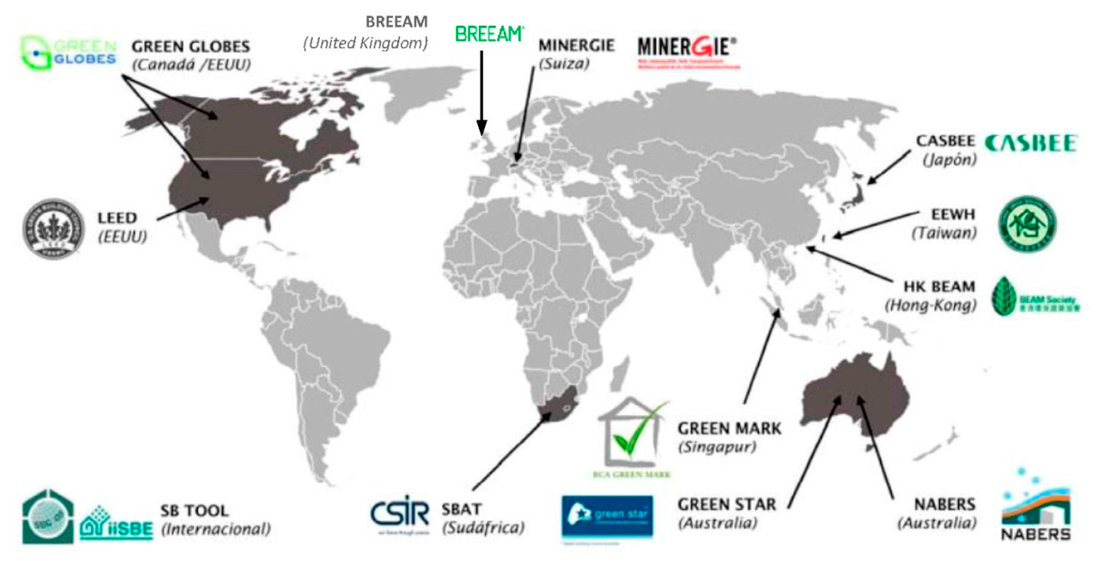
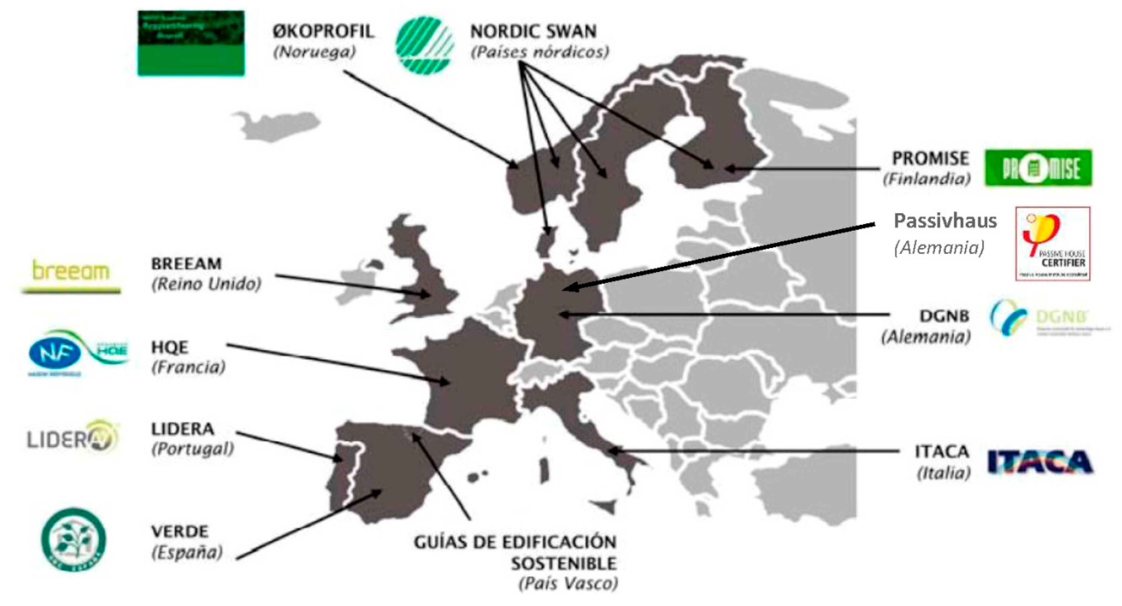
2.1. Energy Certificates

Sustainable architecture is capable of reducing environmental impact based on its design, construction, use, and demolition. According to IHOBE [2], in order to achieve this, the following are necessary: (1) Sustainable systems of assessment, classification, and certification; (2) sustainable building standards; and (3) assessment tools (software). Sustainable assessment systems score buildings based on a series of indicators, which are not necessarily environmental. Sustainable classification systems score each of the environmental aspects and, from the total of these scores, an overall building score is obtained. A sustainable certification or labeling system is a classification system that is carried out by a qualified and authorized consultant. Ultimately, a building is considered efficient if it has elements that permit its sustainable assessment and this is justified through the obtaining of an EPC.

The most important international organizations supporting the certification processes and assessment tools are the World Green Building Council (WGBC), the International Initiative for Sustainable Building Environment (iiSBE) and the Sustainable Building Alliance (SBA).

On a global level, the most frequently used certification methods are the Building Research Establishment’s Environmental Assessment Method (hereinafter, BREEAM) and the Leadership in Energy & Environmental Design certification (hereinafter, LEED). In Figure 1, the most relevant global assessment systems are shown.

The BREEAM system was initially developed in 1988 in the U.K. by the Building Research Establishment (hereinafter, BRE Global) and was launched in 1990 for commercial and residential building assessment. Today its use has been extended to all types of buildings. It is a voluntary and private certification system. The certification system assesses ten categories or topic areas [3]: (1) Management; (2) health and wellbeing; (3) energy; (4) transport; (5) water; (6) materials; (7) waste; (8) land use and ecology; (9) pollution; and (10) innovation. Its final objective is to provide a sustainable label that stimulates the creation of sustainable cities. This method is based on the scoring of distinct categories. The score obtained in each topic area includes an environmental factor which considers the relative importance in each category. The results from each category are combined to obtain an overall score.

LEED certification was developed in 1993 in the U.S., by the Green Building Council. It is a voluntary and private certification system. This certification system assesses eight categories or topic areas [4]: (1) Location and transportation; (2) sustainable sites; (3) water efficiency; (4) energy and atmosphere; (5) materials and resources; (6) indoor environmental quality; (7) innovation; and (8) regional priority. The method used is based on the scoring of distinct categories, with the results of each category adding up to obtain an overall score. LEED certification is available at four progressive levels in accordance with the following scale: LEED Certificate, from 40 to 49 points; LEED Silver, from 50 to 59 points; LEED Gold, from 60 to 79 points; and LEED Platinum with 80 points or more.

The BREEAM and LEED certifications have been developed across the world, with specific stamps existing in almost all countries and with adaptations based on geographic location and building type.

Other certifications appearing in this study are the Comprehensive Assessment System for Building Environmental Efficiency (CASBEE), National Australian Built Environment Rating System (NABERS), Minergie, and GreenMark.

The CASBEE certification was developed in Japan by the Ministry of Land, Infrastructure, Transport, and Tourism, managed by the Japan Green Building Council (JaGBC) and the Japan Sustainable Consortium (JSBC). The CASBEE certification is available at five progressive levels in accordance with the following scale or scoring: Class C (low score) represented by one star; Class B, represented by two stars; Class B+ represented by three stars; Class A with four stars; and Class S (excellent) with five stars.

In Australia, two certification types are used: Green Star and NABERS. Green Star is a voluntary sustainable classification system that was developed by the Green Building Council of Australia. NABERS is promoted by the Australian government and is used to measure the sustainability of commercial buildings and offices.

Minergie is a voluntary certification created in Switzerland in 1994. It is a sustainable classification system used for new and restored buildings with low consumption. In 2001, a stricter Minergie-P classification was established for passive housing. Green Mark is a voluntary certificate that was created in Singapore in January of 2005 to promote sustainable buildings and to create environmental awareness, managed by the Building and Construction Authority (BCA).

In Europe, Directive 2002/91/CE [5], recast as Directive 2010/31/UE [6] implemented a mandatory certification system called the “ABCDEFG qualification”, classifying buildings based on their energy efficiency. It establishes a scale of values that ranges from the letter “A” (best energy qualification) to the letter “G” (worst energy qualification). The assigned letter is based on the quantity of energy consumed (kW/year·m²) and/or the CO₂ emitted by said building during its use. These certificates should be prepared by a competent technician, with the assistance of computerized tools created by relevant bodies of the European governments in order to qualify the energy efficiency of the buildings. Furthermore, upon creation of the certificates, they should be registered in an official public and informative institution.

In Europe, in addition to the mandatory certification, other voluntary standards exist (Figure 2). One example of this is the Passivhaus seal which was created in 1988 in Germany to reduce energy consumption. With this objective, the general directives are based on the creation of buildings with great thermal isolation, control of infiltrations, and good interior air quality, while also taking advantage of solar energy to improve the air conditioning [7].

2.2. Background Information

Numerous studies have found that housing with energy qualifications have a positive premium in the sales and rental price. Other studies, however, have obtained negative or contrary results. For example, Yang [8] obtained a premium of 16% on new housing having a LEED qualification in Portland (United States). On the other hand, Yoshida and Sugiura [9] found a negative premium of 10.80% in housing with a Green Building qualification in Tokyo (Japan).

The purpose of this research is to estimate a representative value (effect size) based on prior studies. To do so, meta-analysis was used, in order to summarize the evidence accumulated in the study. This type of reviews began with Smith and Glass [10], but it was Hedges and Olkin [11] who proposed a methodology. Currently, the meta-analysis is a methodology used in all disciplines in which the study and analysis of the methodology has proliferated [12,13,14,15].

As Hunter and Schmidt [16] indicated, the meta-analysis is intended to integrate the findings from diverse studies so as to detect relationships existing between the same, generating a basis for theory development. Therefore, a meta-analysis in any science is the production of cumulative knowledge, used in all disciplines. Schmidt [17] indicates that meta-analyses may in fact offer more contributions to scientific analysis than primary research studies. According to Eden [18], empirical research increases in value when scientific generalizations may be made based on meta-analyses.

At the date of creation of this study, four documents were found that conduct meta-analyses on the economic price premium of buildings with an energy qualification. The first is a report created by Ankamah-Yeboah and Rehdanz [19] in which a systematic review is conducted, along with a meta-regression with 30 documents (or studies) that include 205 registers (specification of a regression model), to determine the economic price premium of residential and office buildings that are for sale or for rent. They found that buildings with some type of qualification have an average premium of 7.6%. In their results, the authors indicate that energy efficiency of residential buildings is more highly valued in the case of sales markets and for those having voluntary labeling. The opposite is found in office buildings, where the energy qualification of the building is more highly valued in the rental market, as is the seniority of the qualification system. As for the premiums based on geographic location, higher premiums were obtained in Europe as compared to the U.S.

The second document is a report created by Brown and Watkins [20] in which a systematic review was conducted with meta-analysis and meta-regression, based on 17 studies and 20 registers. The results reveal that the housing with an energy qualification has a mean weighed premium of 4.3%. The authors indicate that, given the low number of observations, it is not possible to affirm that there are significant differences based on building location and qualification type.

The third document, Kim et al. [21], conducted a systematic review and a meta-regression of the economic premiums in office rental buildings. They analyzed a selection of nine publications that included 34 registers, finding a significant premium in the rental prices of 14.66%. The authors indicated that other characteristics with the greatest influence on the selection of this type of buildings are location, building characteristics, and contract type.

The last document, Fizaine et al. [22], conducted a systematic review with meta-analysis and meta-regression, to determine the economic premium in the sales price of the housing, using 54 documents which include 79 registers. The authors found that the economic premium varied between 3.5% and 4.5%, once correcting for publication bias. They attributed the dispersion of the results to: 1) Study location (North America, Asia, or Europe); 2) publication type; and 3) whether or not, in the hedonic model, localization variables were included. It should be mentioned that the authors found that, in many of the analyzed documents, standard error values were missing (or t test values or their statistical significance p), values that are necessary to conduct a meta-analysis. Furthermore, in some studies, the estimation of the qualification was carried out using distinct references, hindering comparison between them.

3. Materials and Methods

For the following steps, the criteria from the PRISMA [23,24] declaration were considered, which include: (1) Identification of the studies and information sources, in addition to the strategy of searching for documents with the dates of coverage and document identification (Section 3.1 of this document); (2) eligibility requirements, specifying the inclusion and exclusion criteria from the documents (Section 3.2); (3) baseline data, which describes the collected variables (Section 3.3 and 3.7); (4) data integrity through an assessment of information quality (Section 3.4); (5) document protocol and registry (

Table 1. Set of the 66 documents making up the study, with the 213 registers generated; assessment of the document based on the information provided (Rating) and type of analysis performed, according to Figure 4.

Year	Study	Country	Label	Date Data	En.	Compares	Typology	Sales/Rent	Premium	Reg. Nº	Rating	Analysis
2007	[49]	U.S.	Sustainable indicators	1998–2004	NO	Efficient housing/NOT efficient housing	Single family	Sale	3.98%	1	40.0	A1
2008	[34]	Switzerland	Minergie	1998–2008	NO	Labeled/non-labeled	Single family	Sale	7.00%	2	0.0	A1*
				1998–2008	NO	Labeled/non-labeled	Multifamily	Sale	3.50%	3	0.0	A1*
2008	[28]	Australia	ACTHER S (1–10)	2005	YES	Stars 1–6 (0.5 increment)	Single family	Sale	1.23%	4	45.0	A0
				2006					1.91%	5	45.0	A0
				2005–2006					- Star 1: 1.56% - Star 2: 2.98% - Star 3: 5.90% - Star 4: 6.28% - Star5/6: 6.14%	6	45.0	A0
2010	[50]	Switzerland	Minergie	2002–2010	NO	Labeled/non-labeled	Multifamily	Net Rent	6.00%	7	5.0	A0
								Gross Rent	4.90%	8	5.0	A0
2010	[40]	Japan	Green Label	2005–2008	NO	Labeled/non-labeled	Multifamily	Sale	4.70%	9	37.5	A1
2010	[41]	Japan	Green Building	2002–2009	YES	Labeled/non-labeled	Multifamily	Sale	−5.63%	10	37.5	A1
2011	[51]	Singapore	Green Mark Certified	2005–2009	NO	Labeled/non-labeled	Multifamily	Sale	11.69%	11	37.5	A1
						- GMC - GMG - GMGP - GMPL			- GMC: 12.97% - GMG: 9.64% - GMGP: 9.61% - GMPL: 27.74%	12	27.5	A0
2011	[52]	U.S.	Energy Star	1995–2005	NO	Labeled/non-labeled	Single family	Sale	$8.66/pie2	13	15.0	A0
2011	[53]	Netherlands	ABCDEFG qualification	2008–2009	YES	Qualification: ABC/DEFG (without thermal characteristics) ①	Multiple	Sale	- ABC: 3.70% - DEFG: Ref.	14	37.5	A2
						Qualification: A/B/C/D/E/F/G (without thermal characteristics) ①	Multiple	Sale	- A: 10.2% - B: 5.6% - C: 2.2% - D: Ref. - E: −0.5% - F: −2.5% - G: −5.1%	15	37.5	A2
						Qualification: ABC/DEFG (with thermal characteristics) ①	Multiple	Sale	- ABC: 3.60% - DEFG: Ref.	16	37.5	A2
						Qualification: A/B/C/D/E/F/G (with thermal characteristics) ①	Multiple	Sale	- A: 10.2% - B: 5.5% - C: 2.1% - D: Ref. - E: −0.5% - F: −2.3% - G: −4.8%	17	37.5	A2
2012	[42]	U.S.	Residential Green Building Program	2002–2009	YES	Labeled/non-labeled	Single Family	Sale	2.00%	18	37.5	A1
2012	[54]	Singapore	Green Mark	2000–2010	NO	Labeled/non-labeled	Multifamily	Sale	4.00%	19	37.5	A1
2012	[55]	U.S.	Energy Star, LEED o Green	2007–2012	NO	Labeled/non-labeled	Single Family	Sale	11.80%	20	40.0	A1
2012	[56]	U.S.	EarthCraft House	2007–2010	NO	Labeled/non-labeled	Single Family	Sale	7.98%	21	47.5	A1
2012	[30]	China	Google Green Index	2011	NO	Labeled/non-labeled	Multifamily	Sale	−0.25%	22	30.0	A0
				2003–2008	NO	Labeled/non-labeled		Sale	0.35%	23	30.0	A1*
2013	[57]	Germany	ABCDEFG qualification	2008–2010	NO	Qualification: B/C/D/E/F/G	Multifamily	Rent	- B: 12.5% - C: 12.7% - D: 15% - E: 14.7% - F: 3.2% - G: Ref.	24	35.0	A0
2013	[58]	Switzerland	Sustainable indicators	2010–2011	NO	Different items	Multifamily	Rent	- Flexibility: 1.0% - Energy and water efficiency: 11% - Accessibility and mobility: −4% - Security and protection: 9% - Health-comfort: 9%	25	20.0	A0
2013	[59]	United Kingdom	ABCDEFG qualification	1995–2012	YES	Qualification AB/C/D/E/F/G	Single family (Full sample.)	Sale	- AB: 13.8% - C: 9.91% - D: 7.6% - E: 6.55% - F: −5.96% - G: Ref.	26	40.0	A2
						Qualification AB/C/D/E/F/G	Single family (Detached)	Sale	- AB: 2.13% - C: 1.29% - D: 1.3% - E: 0.26% - F: 0.00% - G: Ref.	27	37.5	A2*
						Qualification AB/C/D/E/F/G	Single family (Semi-detached)	Sale	- AB: 10.1% - C: 7.68% - D: 6.75% - E: 5.12% - F: 4.03% - G: Ref.	28	37.5	A2*
						Qualification AB/C/D/E/F/G	Single family (Terraced)	Sale	- AB: 18.2% - C: 15.5% - D: 13.5% - E: 11.4% - F: 8.16% - G: Ref.	29	40.0	A2*
						Qualification AB/C/D/E/F/G	Multifamily (Flat)	Sale	- AB: 11.6% - C: 10.4% - D: 9.33% - E: 8.03% - F: 5.55% - G: Ref.	30	37.5	A2*
						Qualification AB/C/D/E/F/G	Single family (Detached dense)	Sale	- AB: 9.17% - C: 7.79% - D: 7.49% - E: 5.98% - F: 5.03% - G: Ref.	31	37.5	A2*
						Qualification AB/C/D/E/F/G	Single family (Detached sparse)	Sale	- AB: −4.94% - C: −3.85% - D: −2.01% - E: −1.55% - F: −2.05% - G: Ref.	32	37.5	A2*
2013	[43]	Sweden	ABCDEFG qualification	2009	YES	Energy efficiency	Single Family	Sale	- 4.41	33	40.0	A1
2013	[25]	Ireland	ABCDEFG qualification	2008–2012	YES	Qualification: A/B/C/D/E/F/G	Multiple	Rent	- A: 1.8% - B: 3.9% - C: −0.6% ② - D: Ref. - E: −1.9% ② - F: −3.2% ② - G: −2.3% ②	34	17.5	A0
				2008–2013		Labeled/non-labeled	Multiple	Rent	−0.50%	35	17.5	A0
				2008–2012		Qualification: A/B/C/D/E/F/G	Multiple	Sale	- A: 9.3% - B: 5.2% - C: 1.7% - D: Ref. - E: −0.4% ② - F: −10.6% ② - G: −2.3% ②	36	17.5	A2
				2008–2013		Labeled/non-labeled	Multiple	Sale	1.30%	37	17.5	A1
2013	[60]	China. Yuen Long District	Green Building Council (HKGBC)	-	NO	Labeled/non-labeled	Multifamily	Sale	7.05%	38	45.0	A1
		China. Quarry Bay District							2.98%	39	45.0	A1
2013	[26]	Austria	ABCDEFG qualification	2012	YES	Labeled/non-labeled	Multiple	Rent	4.41%	40	30.0	A0
		Austria						Sale	8.03%	41	30.0	A1
		Belgium. Brussels	ABCDEFG qualification	2012	YES	Labeled/non-labeled	Multiple	Rent	2.60%	42	25.0	A0
		Belgium. Wallonia							1.50%	43	25.0	A0
		Belgium. Flanders							3.20%	44	30.0	A0
		Belgium. Brussels	ABCDEFG qualification	2012	YES	Labeled/non-labeled	Multiple	Sale	2.90%	45	30.0	A1
		Belgium. Wallonia							5.40%	46	25.0	A1
		Belgium. Flanders							4.30%	47	32.5	A1
		France. Marseille	ABCDEFG qualification	2011–2012	YES	Labeled/non-labeled	Multiple	Sale	4.34%	48	30.0	A1
		France. Lille							3.24%	49	30.0	A1
		Ireland	ABCDEFG qualification	2008–2012	YES	Labeled/non-labeled	Multiple	Rent	1.15%	50	32.5	A0
									1.52% ③	51	32.5	A0
		Ireland						Sale	2.83%	52	32.5	A1
									1.69% ③	53	32.5	A1
		United Kingdom	ABCDEFG qualification	2012	YES	Labeled/non-labeled	Multiple	Sale	1.04%	54	25.0	A1
2013	[61]	Japan	CASBEE	2005–2010	YES	Labeled/non-labeled	Multifamily	Sale	5.84%	55	37.5	A1
2013	[62]	U.S. Research Triangle	Energy Star	2009–2011	NO	Labeled/non-labeled	Single Family	Sale	2.40%	56	32.5	A1
		U.S. Austin	Energy Star	2008–2011					3.80%	57	32.5	A1
		U.S. Austin	Local green certification	2008–2011					14.30%	58	32.5	A1
		U.S. Portland	Energy Star	2005–2011					3.60%	59	35.0	A1
		U.S. Portland	Local green certification	2005–2011					8.00%	60	35.0	A1
2013	[8]	U.S.	LEED	2009–2012	NO	Labeled/non-labeled	Multifamily	Sale	5.80%	61	35.0	A1
							Single Family	Sale	16.00%	62	35.0	A0
2014	[63]	Sweden	ABCDEFG qualification	2009–2010	YES	Energy efficiency	Multifamily	Sale	- Total: 6% - R. high: −6% - R. Md.: −37% - R. low: −14%	63	30.0	A0
2014	[64]	Singapore	Green Mark	2000–2010	NO	Labeled/non-labeled	Multifamily	Sale	4.60%	64	42.5	A1
2014	[65]	Japan	Green Building	2001–2011	YES	Stars 2-3	Multifamily	Sale	1.60%	65	47.5	A0
2014	[66]	U.S.	Energy Star	2007–2012	NO	Labeled/non-labeled	Multiple	Sale	5.30%	66	40.0	A1
2014	[67]	Canada	LEED	2013	NO	Labeled/non-labeled	Multifamily	Sale	−2.49% ②	67	35.0	A1
2015	[68]	Italy	ABCDEFG qualification	2013	YES	Qualification: A/B/C/D/E/F/G	Single Family	Sale	- A: 21.9% - B: 20.2% - C: 17.4% - D: 17.1% - E: 9.5% - F: 2.3% ② - G: Ref.	68	30.0	A2
2015	[44]	Ireland (North)	ABCDEFG qualification	-	YES	Labeled/non-labeled	Single Family	Sale	0.40	69	45.0	A1
2015	[69]	Canada	LEED	2006–2014	NO	Labeled/non-labeled	Multifamily	Sale	- Gold: 12.20%	70	35.0	A1
									- Silver: 6.20%	71	35.0	A0
2015	[70]	Italy	ABCDEFG qualification	2012	YES	Qualification B/C/D/E/F/G	Multifamily	Sale	- B: Ref. - C: −3% ② - D: −10% ② - E: −6% ② - F: −14% ② - G: −10%	72	40.0	A2
2015	[71]	U.S.	LEED	2007–2013	NO	Labeled/non-labeled	Multifamily	Sale	3.80%	73	35.0	A1
2015	[36]	United Kingdom	ABCDEFG qualification	1995–2012	YES	Qualification AB/C/D/E/F/G	Multifamily	Sale	- AB: 5.0% - C: 1.8% - D: Ref. - E: −0.07% - F: −0.09% - G: −6.8%	74	40.0	A2
						Qualification AB/C/D/E/F/G	Single Family (Semi-detached)	Sale	- AB: 0.08% ② - C: 0.05% - D: Ref. - E: −1.30% - F: −2.3% - G: −6.5%	75	40.0	A2*
						Qualification AB/C/D/E/F/G	Single Family (Terraced)	Sale	- AB: 4.5% - C: 1.5% - D: Ref. - E: −1.9% - F: −4.6% - G: −12.1%	76	40.0	A2*
						Qualification AB/C/D/E/F/G	Multifamily (Flat)	Sale	- AB: 1.6% - C: 0.8% - D: Ref. - E: −1.4% - F: −2.9% - G: −7.2%	77	37.5	A2*
						Qualification AB/C/D/E/F/G	Single family (Detached dense)	Sale	- AB: 2.0% - C: 0.2% - D: Ref. - E: −1.2% - F: −2.0% - G: −7.0%	78	37.5	A2*
						Qualification AB/C/D/E/F/G	Single family (Detached sparse)	Sale	- AB: 11.1% - C: 3.1% - D: Ref. - E: 0.8% - F: 0.9% - G: 1.8%	79	37.5	A2*
						Labeled/non-labeled	Multifamily	Sale	0.06%	80	50.0	A1
2015	[72]	Portugal	ABCDEFG qualification	2015	YES	Qualification ABC/D/EFG	Multifamily	Sale	- ABC: 5.94% - D: Ref. - EFG: −4.03%	81	17.5	A2
		Portugal. Lisbon/Oporto				Qualification ABC/D/EFG	Single family	Sale	- ABC: 10.6% - D: Ref. - EFG: −0.63%	82	15.0	A2*
2015	[37]	U.S.	Some AEGB, ES or EFL	2008–2012	NO	Labeled/non-labeled	Single family	Sale	5.00%	83	32.5	A0
			Austin Energy (AEGB)						6.00%	84	32.5	A1
			Energy Star						1.00%	85	32.5	A1
			Environments for Living (EFL)						9.00%	86	32.5	A1
2015	[9]	Japan	Green Building	2002–2009	YES	Labeled/non-labeled	Multifamily	Sale	−10.80%	87	37.5	A1*
2016	[73]	U.S.	LEED	2000–2012	NO	Labeled/non-labeled	Single family	Rent	7.00%	88	35.0	A0
2016	[74]	U.S.	Energy Star	1998–2009	NO	Labeled/non-labeled	Single family	Sale	4.94%	89	30.0	A1
2016	[75]	Netherlands	ABCDEFG qualification	2008–2013	YES	Labeled/non-labeled	Multiple	Sale	−0.80%	90	37.5	A1
						Labeled/non-labeled			−0.70%	91	37.5	A1
						Qualification AB/CDEFG (with thermal characteristics) ①			- AB: 1.3% - CDEFG: −0.8%	92	37.5	A2
						Qualification A/B/C/D/E/F/G (with thermal characteristics) ①			- A: 5.6% - B: 1.1% - C: −0.2% - D: −0.8% - E: −1.4% - F: −1.6% - G: −0.8% - NT: Ref.	93	37.5	A2
2016	[39]	Spain	ABCDEFG qualification	2013	YES	Qualification ABC/DEFG	Multifamily	Sale	- ABC: 9.8% - DEFG: Ref.	94	27.5	A2
						Qualification ABCD/EFG			- ABCD: 5.40% - EFG: Ref.	95	27.5	A2
2016	[76]	Japan	Green Labeling System for Condominiums	2003–2011	YES	Labeled/non-labeled	Multifamily	Sale	4.82%	96	47.5	A1
							Multifamily	Sale	5.89%	97	45.0	A1
2016	[35]	United Kingdom	ABCDEFG qualification	2003–2014	YES	Qualification AB/C/D/E/F/G	Multifamily	Sale	- AB: 11.3% - C: 2.06% - D: Ref. - E: −2.09% - F: −4.73% - G: −7.17%	98	37.5	A2
							Single family (Detached)	Sale	- AB: −1.99% ② - C: 0.20% ② - D: Ref. - E: −1.74% - F: −4.42% - G: −4.99%	99	32.5	A2*
							Single family (Detached rural)	Sale	- AB: −1.81% ② - C: −0.16% ② - D: Ref. - E: −0.58% - F: −3.05% - G: −5.91%	100	25.0	A2*
							Single family (Detached urban)	Sale	- AB: −2.0% ② - C: 0.27% ② - D: Ref. - E: −2.14% - F: −6.87% - G: −5.27%	101	35.0	A2*
							Single family (Semi-detached)	Sale	- AB: 8.24% - C: 0.40% ② - D: Ref. - E: −2.04% - F: −5.51% - G: −8.32%	102	35.0	A2*
							Single family (Terraced)	Sale	- AB: 17.1% - C: 2.34% - D: Ref. - E: −3.61% - F: −9.45% - G: −14.0%	103	37.5	A2*
							Multifamily (Flat)	Sale	- AB: 3.55% - C: 3.88% - D: Ref. - E: −8.24% - F: −10.5% - G: −15.0%	104	30.0	A2*
					YES	Labeled/non-labeled	Multifamily	Sale	4.32%	105	47.5	A1
2016	[31]	Denmark	ABCDEFG qualification	2007–2010	YES	Qualification ABC/DEFG	Single family before 1 July 2010	Sale	- ABC: 2.40% - DEFG: Ref.	106	37.5	A2
				2010–2012			Single family after 1 July 2010	Sale	- ABC: 10.10% - DEFG: Ref.	107	37.5	A2
				2007–2012		Qualification AB/C/D/E/F/G	Single family before 1 July 2010	Sale	- AB: 6.6% - C: 0.2% - D: Ref. - E: −1.5% - F: −3.5% - G: −9.3%	108	37.5	A2
				2010–2012			Single family after 1 July 2010	Sale	- AB: 6.2% - C: 5.1% - D: Ref. - E: −5.4% - F: −12.9% - G: −24.3%	109	37.5	A2
2016	[77]	Switzerland	Minergie	-	NO	Labeled/non-labeled	Multiple	Rent	15.08%	110	35.0	A0
							Multiple	Sale	21.5%	111	42.5	A1*
2016	[78]	Spain	ABCDEFG qualification	2014	YES	Labeled/non-labeled	Multifamily	Sale	1.02%	112	35.0	A1
						Qualification: A/B/C/D/E/F/G			- A: 9.62% - D: 3.87% - F: Ref. - G: 5.4%	113	25.0	A2
2016	[79]	Ireland	ABCDEFG qualification	2009–2014	YES	Labeled/non-labeled	Multiple	Sale	1%	114	30.0	A1
						Qualification A3/B1/B2/B3/C1/C2/C3/D1/D2/E1/E2/F/G			- A3: 2.8% ② - B1: −28.2% ② - B2: −1.3% ② - B3: 1.7% ② - C1: Ref. - C2: −3.9% ② - C3: −0.8% ② - D1: −1.1% ② - D2: −4.6% - E1: −3.4% ② - E2: −7% - F: −4.4% ② - G: −12.8%	115	30.0	A2
2016	[80]	China	Chinese Green Building Label	2013	NO	Labeled/non-labeled	Multifamily	Sale	6.66%	116	20.0	A1
2017	[81]	U.S.	Residential Green Building Program	2002–2009	YES	Labeled/non-labeled	Single family	Sale	2.27%	117	32.5	A1
2017	[82]	Belgium	ABCDEFG qualification	2010–2014	YES	Qualification ABC/DE/FG	Single family	Rent	- ABC: 6.8% - DE: 1.9% - FG: Ref.	118	17.5	A0
2017	[83]	China	BEAM Plus	2012–2014	NO	Classification: Gold, silver and bronze	Multifamily	Sale	4.40%	119	30.0	A0
						Classification: low		Sale	−5.90%	120	20.0	A0
						Classification: Gold, silver and bronze	Single family	Sale	6.20%	121	30.0	A0
2017	[33]	U.S. Atlanta	-	2016–2017	NO	Features that enhance the EE	Single family	Rent	14.10%	122	0.0	A0
		U.S. Chicago							13.40%	123	0.0	A0
		U.S. Washington DC							6.90%	124	0.0	A0
		U.S. Indianapolis							−0.50%	125	0.0	A0
		U.S. Las Vegas							5.30%	126	0.0	A0
		U.S. Miami							0.60%	127	0.0	A0
		U.S. Minneapolis							6.00%	128	0.0	A0
		U.S. Oklahoma							5.60%	129	0.0	A0
		U.S. Philadelphia							6.30%	130	5.0	A0
		U.S. San Francisco							7.20%	131	0.0	A0
		U.S. Atlanta	-	2016–2017	NO	Features that enhance the EE	Multifamily	Rent	16.10%	132	0.0	A0
		U.S. Chicago							13.90%	133	0.0	A0
		U.S. Washington DC							6.60%	134	0.0	A0
		U.S. Indianapolis							−3.20%	135	0.0	A0
		U.S. Las Vegas							2.30%	136	0.0	A0
		U.S. Miami							−0.10%	137	0.0	A0
		U.S. Minneapolis							5.90%	138	0.0	A0
		U.S. Oklahoma							2.60%	139	0.0	A0
		U.S. Philadelphia							5.20%	140	5.0	A0
		U.S. San Francisco							5.60%	141	0.0	A0
2017	[84]	Germany	ABCDEFG qualification	2011–2014	YES	Energy consumption	Multifamily	Rent	−0.02%	142	35.0	A0
								Sale	−0.05%	143	35.0	A1*
2017	[85]	France. Grande Couronne	ABCDEFG qualification	2016	YES	Qualification AB/C/D/E/FG	Single family	Sale	- D: Ref. - E: −2% - FG: −6%	144	30.0	A2
		France. Petite Couronne							- C: 5% - D: Ref. - FG: −7%	145	30.0	A2
		France. Hauts de France							- AB: 6% - C: 5% - D: Ref. - E: −4% - FG: −9%	146	10.0	A2
		France. Normandie							- AB: 8% - C: 6% - D: Ref. - E: −3% - FG: −10%	147	10.0	A2
		France. Grand Est							- C: 5% - D: Ref. - E: −4% - FG: −14%	148	10.0	A2
		France. Bretagne							- AB: 11% - C: 6% - D: Ref. - E: −8% - FG: −13%	149	10.0	A2
		France. Pays de la Loire							- AB: 9% - C: 4% - D: Ref. - E: −6% - FG: −13%	150	10.0	A2
		France. Centre Val de Loire							- AB: 10% - C: 5% - D: Ref - E: −7% - FG: −14%	151	10.0	A2
		France. Bourgogne Franche-Comté							- C: 4% - D: Ref. - E: −6% - FG: −15%	152	10.0	A2
		France. Nouvelle Aquitaine							- AB: 13% - C: 6% - D: Ref. - E: −6% - FG: −16%	153	10.0	A2
		France. Auvergne Rhone-Alpes							- AB: 11% - C: 5% - D: Ref. - E: −3% - FG: −7%	154	10.0	A2
		France. Occitanie							- AB: 10% - C: 6% - D: Ref. - E: −7% - FG: −17%	155	10.0	A2
		France. Provence-Alpes-Côte d’Azur							- AB: 7% - C: 3% - D: Ref. - E: −3% - FG: −10%	156	10.0	A2
		France. Grande Couronne					Multifamily	Sale	- AB: 8% - D: Ref.	157	30.0	A2
		France. Grand Est							- C: 4% - D: Ref.	158	10.0	A2
		France. Pays de la Loire							- AB: 6% - D: Ref.	159	10.0	A2
		France. Centre Val de Loire							- AB: 19% - D: Ref.	160	10.0	A2
		France. Bourgogne Franche-Comté							- AB: 19% - C: 5% - D: Ref.	161	10.0	A2
		France. Nouvelle Aquitaine							- AB: 11% - D: Ref. - FG: −7%	162	10.0	A2
		France. Auvergne Rhone-Alpes							- AB: 10% - C: 3% - D: Ref.	163	10.0	A2
		France. Occitanie							- AB: 14% - C: 3% - D: Ref. - E: −4% - FG: −6%	164	10.0	A2
		France. Provence-Alpes-Côte d’Azur							- AB: 3% - D: Ref. - FG: −10%	165	10.0	A2
2017	[29]	Norway	ABCDEFG qualification	2014	YES	Qualification: A/B/C/D/E/F/G	Multiple	Sale	- A: 4.3% ② - B: 18.9% - C: 12.2% - D: 7.5% - E: 0.5% ② - F: Ref. - G: 5.4%	166	25.0	A2
				2000–2014	YES	Qualification: A/B/C/D/E/F/G	Multiple	Sale	- B: 24.6% - C: 11.5% - D: 9.7% - E: 3.0% ② - F: Ref. - G: 2.7%	167	25.0	A2
2017	[86]	U.S.	Home Energy Rebate	2008–2015	NO	Stars 1-4	Single family	Sale	4.20%	168	30.0	A0
2017	[87]	Canada	LEED	2013	NO	Labeled/non-labeled	Multifamily	Sale	−1.08% ②	169	35.0	A1
2017	[32]	U.S. Austin	Energy Star	2008–2011	NO	Labeled/non-labeled	Single family	Sale	0.60%	170	37.5	A1
		U.S. Austin	Austin Energy (AEGB)	2008–2011					8.20%	171	37.5	A1
		U.S. North Carolina	Energy Star	2009–2011					2.70%	172	32.5	A1
		U.S. Portland	Energy Star	2005–2011					3.50%	173	35.0	A1
		U.S. Portland	Earth Advantage New Homes	2005–2011					8.02%	174	35.0	A1
2018	[88]	Belgium	ABCDEFG qualification	2010–2014	YES	Qualification ABC/DE/FG	Single family	Rent	- ABC: 6.9% - DE: 1.9% - FG: Ref	175	17.5	A0
					YES	Qualification B/C/D/E/F/G	Single family	Rent	- B: 8.1% - C: 5.7% - D: 1.7% - E: 0.3% ② - F: −1.8% - G: Ref.	176	17.5	A0
2018	[27]	Australia	ACTHER S (1-10)	2011–2017	YES	Stars 1-10	Single family	Rent	- EER 0: −2.81% - EER 1: −2.38% - EER 2: −1.06% - EER 3: Ref. - EER 4: 0.06% - EER 5: 3.48% - EER 6: 3.61% - EER 7: 2.63% - EER8: −10:3.5%	177	27.5	A0
				2011–2016				Sale	- EER 0: −3.10% - EER 1: −2.72% - EER 2: −1.81% - EER 3: Ref. - EER 4: 0.42% - EER 5: 2.0% - EER 6: 2.37% - EER 7: 9.36% - EER8: −10:2.7%	178	27.5	A0
2018	[45]	France. Grande Couronne	ABCDEFG qualification	2017	YES	Qualification AB/C/D/E/FG	Single family	Sale	- AB: 9% - D: Ref. - FG: −4%	179	30.0	A2
		France. Petite Couronne							- AB: 8% - C: 3% - D: Ref. - E: −2% - FG: −6%	180	30.0	A2
		France. Hauts de France							- AB: 8% - C: 5% - D: Ref. - E: −3% - FG: −11%	181	10.0	A2
		France. Normandie							- AB: 9% - C: 6% - D: Ref. - E: −4% - FG: −10%	182	10.0	A2
		France. Grand Est							- AB: 11% - C: 5% - D: Ref. - E: −7% - FG: −15%	183	10.0	A2
		France. Bretagne							- AB: 14% - C: 7% - D: Ref. - E: −7% - FG: −14%	184	10.0	A2
		France. Pays de la Loire							- AB: 11% - C: 7% - D: Ref. - E: −5% - FG: −16%	185	10.0	A2
		France. Centre Val de Loire							- AB: 10% - C: 6% - D: Ref. - E: −7% - FG: −14%	186	10.0	A2
		France. Bourgogne Franche-Comté							- AB: 6% - C: 5% - D: Ref. - E: −6% - FG: −14%	187	10.0	A2
		France. Nouvelle Aquitaine							- AB: 12% - C: 7% - D: Ref. - E: −7% - FG: −17%	188	10.0	A2
		France. Auvergne Rhone-Alpes							- AB: 10% - C: 4% - D: Ref. - E: −4% - FG: −9%	189	10.0	A2
		France. Occitanie							- AB: 10% - C: 6% - D: Ref. - E: −6% - FG: −16%	190	10.0	A2
		France. Provence-Alpes-Côte d’Azur							- AB: 9% - C: 3% - D: Ref. - E: −4% - FG: −9%	191	10.0	A2
		France. Petite Couronne							- AB: 9% - C: 4% - D: Ref. - FG: −3%	192	30.0	A2
		France: Grande Couronne							- AB: 13% - D: Ref. - E: −2%	193	30.0	A2
		France. Hauts de France							- AB: 9% - D: Ref. - FG: −4%	194	30.0	A2
		France. Grand Est							- AB: 16% - C: 5% - D: Ref. - FG: −4%	195	10.0	A2
		France. Bretagne							- AB: 6% - D: Ref.	196	10.0	A2
		France. Pays de la Loire							- AB: 10% - D: Ref. - FG: −6%	197	10.0	A2
		France. Bourgogne Franche-Comté							- C: 12% - D: Ref.	198	10.0	A2
		France. Nouvelle Aquitaine							- AB: 11% - C: 4% - D: Ref. - E: −5% - FG: −9%	199	10.0	A2
		France. Auvergne Rhone-Alpes							- AB: 14% - C: 6% - D: Ref.	200	10.0	A2
		France. Occitanie							- AB: 22% - C: 6% - D: Ref. - E: −3% - FG: −7%	201	10.0	A2
		France. Provence-Alpes-Côte d’Azur							- AB: 6% - C: 2% - D: Ref. - E: −3% - FG: −10%	202	10.0	A2
2018	[38]	U.S.	EarthCraft House	2007–2010	NO	Labeled/non-labeled	Single family	Sale	12.20%	203	35.0	A1
			Energy Star						8.50%	204	35.0	A1
2019	[89]	Germany	ABCDEFG qualification		YES	Qualification A/B/C/D/E/F/G/H/NT	Single family	Rent	- A+: 0.9% - A: 1.4% - B: 0.9% - C: 0.2% - E: 0% - F: −0.1% - G: −0.3% - H: −0.5% - NT: Ref.	205	35.0	A0
2019	[90]	Spain	ABCDEFG qualification		YES	Qualification ABC/D/E/F/G	Multifamily	Sale	- ABC: −6.3% - D: 1.9% ② - E: 1.1% - F: 1.8% - G: Ref.	206	35.0	A2
2019	[91]	Spain	ABCDEFG qualification	2016	YES	Continuous variable	Multifamily	Sale	1.54%	207	27.5	A0
		Spain. Alicante							−1.0%	208	27.5	A0
		Spain. Barcelona							2.0%	209	27.5	A0
		Spain. Valencia							3.0%	210	27.5	A0
		Spain. Alicante				Qualification A/C/D/E/F/G			- A: 8% - C: −23.5% - D: 2.0% ② - E: −5.0% - F: −5.0% - G: Ref.	211	25.0	A2
		Spain. Barcelona				Qualification A/C/D/E/F/G			- A: 10.0% - C: −6% - D: 7.0% - E: 2.0% - F: 10% ② - G: Ref.	212	25.0	A2
		Spain. Valencia				Qualification A/C/D/E/F/G			- A: 29.0% - C: 18.0% ② - D: 16.0% - E: 4.0% - F: −2.0% ② - G: Ref.	213	25.0	A2

Notes: En.: Enforceability. Reg. Nº.: Register number. ① Thermal characteristics: Heating, outside and insulating maintenance. ② The value obtained is not significant (p > 0.05). ③ Considers the effects of the urban areas. A0: The register is not used in the subsequent analyses. A1: Analysis-1, registers that analyze the impact on the prices of housing with an EPC as compared to housing that is not qualified. A2: Analysis-2, registers that analyze the impact on the sales prices in housing with ABCDEFG qualifications. A1* or A2*: Registers that were discarded for having atypical values. Source: Author’s own creation.

); (6) description of selection bias (Section 4.1.2); (7) results specification, effect size according to the method used (Section 4.1.4); and (8) description of additional analysis methods (Section 4.1.5).

The five first steps are summarized in a Flow Diagram (Section 3.5).

3.1. Search and Selection Criteria

Document selection was conducted in pairs, from January 2018 until late April 2019, via: (1) Consultations of distinct databases (Elsevier ScienceDirect Complete, Springer, LexisNexis Academic, JSTOR, ProQuest Research, Munich Personal RePEc Archive, and Google Scholar); (2) by authors specializing in the “Green Premium” area; and (3) consultations of bibliographic references of the reviewed works. The following key words were used: Energy performance certificate, building energy efficiency rating, valuing building energy labels, building value and energy efficiency, energy efficiency premium. A total of 96 documents were collected, consisting of 71 journal articles, 2 book chapters, 3 congresses, 15 reports, and 5 Master’s theses.

3.2. Selection Criteria

In order to compare and classify the results obtained from the analyzed documents, certain selection criteria were established so as to obtain a homogenous and comparable database, thus permitting reasonable generalization. The following criteria are used: (1) The document analyzes the price premium that is produced based on the existence of the energy qualification; (2) the calculation of the premium was conducted with a hedonic price model (HPM) using a semi-logarithmic functional form; (3) there is an analysis of the impact in residential buildings; and (4) a sales market is considered. Studies using neuronal network models, multi-level analysis, etc., were discarded, as were studies of residential rental markets and the entire commercial or office building market.

Following a reading of the summary of the 96 initially selected documents, it was found that 30 of these examined the effect of the premium on a rental or sales price for commercial or office buildings; therefore, they were discarded since they do not comply with selection criteria number 3 described above. As for the 66 remaining documents, all of them analyzed the effect of the premium on the sales or rental price of the residential buildings. After reading the documents, it was found that in each study one or more registries existed to determine the price premium (a register corresponds to a specification of a regression model). The existence of more than one registry depended on the following: (1) The price premium was analyzed based on the commercialization generating one model for sales and another for rental (for example, [25,26,27]); (2) the price premium of data sets from distinct years was analyzed, thereby generating a registry for each year [28,29,30,31]; (3) the models examined the price premium in distinct cities [26,32,33]; (4) the price premium of the housing was analyzed based on construction type (single or multi-family) [34,35,36]; (5) within the study, distinct types of EPC were analyzed [32,37,38]; (6) different qualification groups were analyzed [31,39]; and (7) the price premium was analyzed by comparing whether or not it had certification [40,41,42,43,44], and furthermore, the premium generated upon changing from one value to another within the EPC value scale was analyzed [25,36,45].

Therefore, of the 66 documents consulted, 213 distinct registers were generated (Figure 3 and Table 1), including studies on buildings that were both for sale and for rent. In a subsequent phase, the registers related to rental housing were discarded (see Section 3.5).

3.3. Measure of Effect

The price premium in the sale of housing with an EPC is measured with the non-standardized regression coefficient β and the squared standardized error, as included in each of the registers. All of the registers included the β coefficient, but certain types of data were not included in the document, such as: The standard error, the sample size, etc. When it was possible to contact the study authors, unavailable data were requested, and on other occasions, they were calculated, as in the case of standard error, based on the β coefficient and sample size [46], using Equation (1).

$$SE=\frac{\beta }{\sqrt{\beta xN}},$$

(1)

where β is the non-standardized regression coefficient and N is the sample size.

3.4. Assessment of the Quality of the Information Available in the Studies

According to Martín Vallejo [47], the documents collected for a meta-analysis, due to their different qualities and origins, may present contradictory results. Therefore, the quality may be assessed by items referring to: The study, the statistical data, or the results presentation. In this document, the quality is assessed in accordance with the statistical analyses, such as effect size and statistical power size of the models provided in each study. In order to obtain the effect size and the statistical power, the GPower program (version 3.1) was used [48]. It was found that the statistical power for all of the documents is near or equal to 1. Therefore, the quality of the studies was not used in the assessment. However, Cohen’s f² ranged between 0.08 and 11.50, so it was used as a quality criteria [21].

$$f^2=\frac{R^{2}fin}{1-R^{2}fin},$$

(2)

where R²fin equals the adjusted R², and when this is not available, the R² is used.

The following scoring criteria were used:

• If the document offers information on:
  • The standard error (SE), it is scored with a 10;
  • The Student’s t test, it is scored with a 10;
  • The sample size and these values are between: 1000–10,000; 10,000–100,000, or are greater than 100,000, it is scored with a 5.0, 7.5 or 10, respectively; if the study does not report on the sample size or if it is less than 1000, it is scored with a 0; and
  • The coefficient of determination, if reporting the R²adj, it is scored with a 10; if the R² is provided, it is scored with a 5;
• If the effect size (f²) is greater than 0.35, 0.50, or 0.8, it is scored with a 5, 7.5, or 10, respectively, if not, or if it is lower than 0.35, it is scored with a 0.

The score resulting from the studies may be checked in the “Rating” column of Table 1.

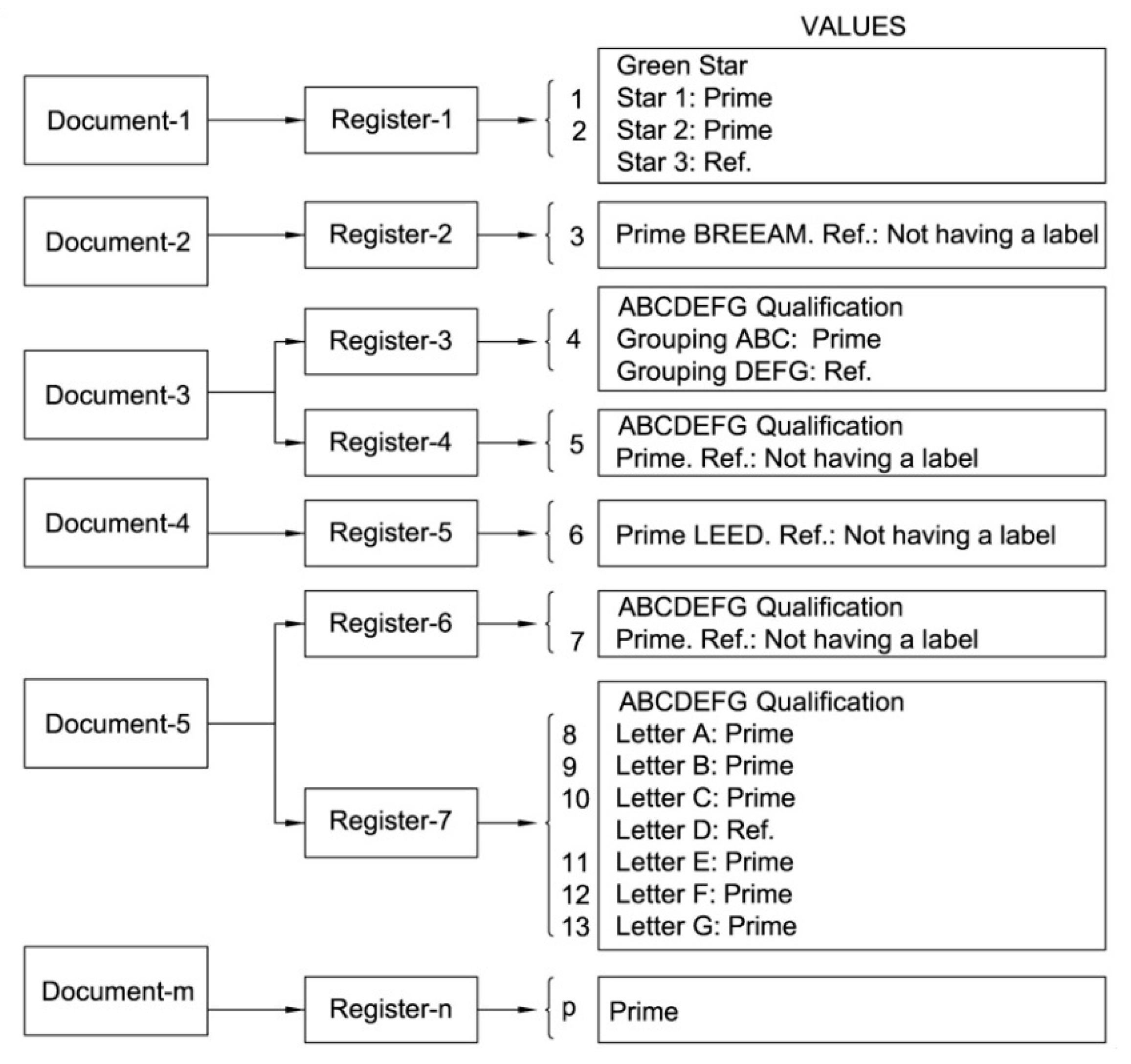
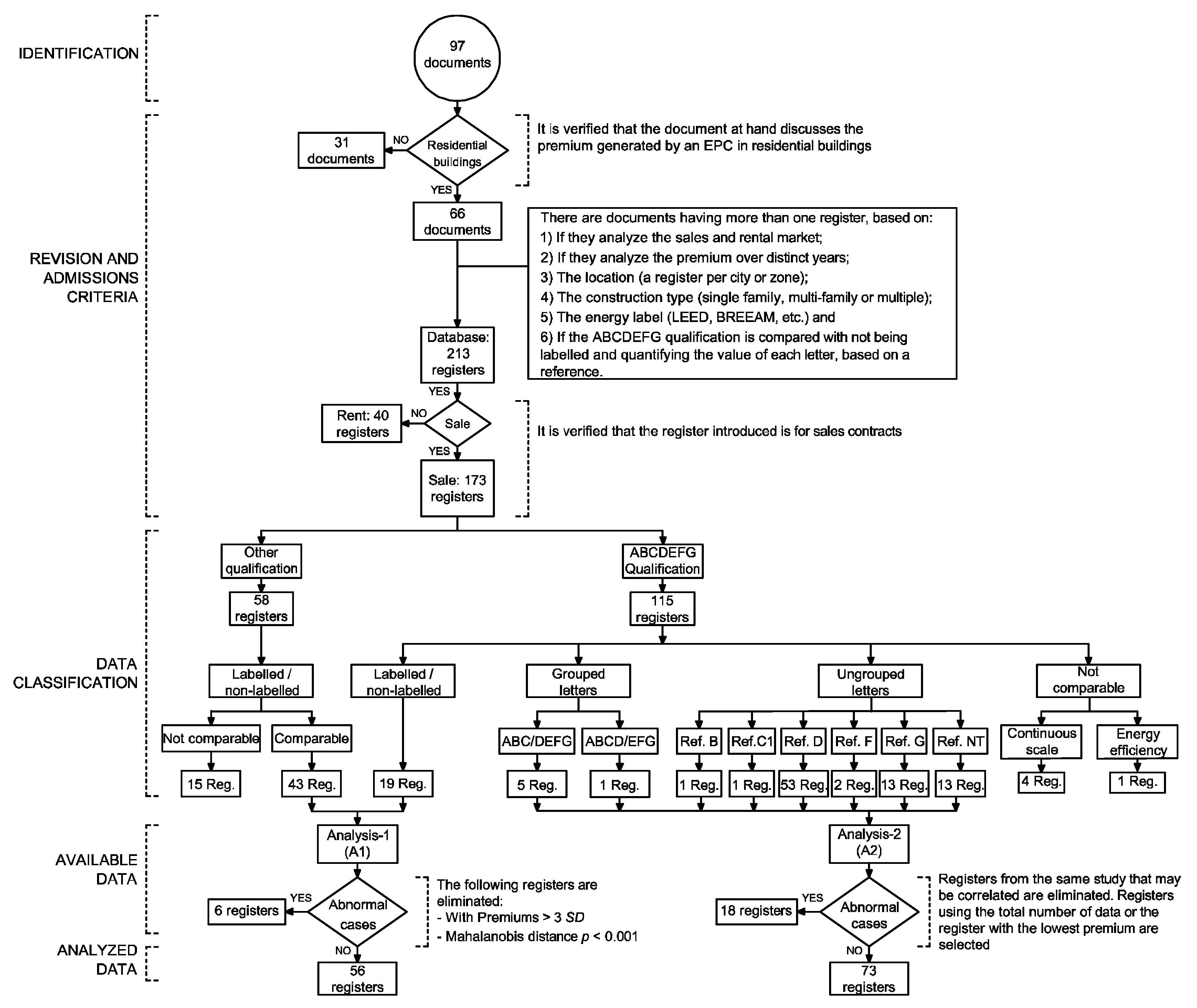
3.5. Data Classification

Of these 213 registers, those related to rentals were discarded, leaving 173 registers that examine the effect of the sales price premium for the housing with an EPC, which are those complying with selection criteria 4) indicated in Section 3.2. The registers are classified based on EPC type: (1) ABCDEFG qualification (115 registers) and (2) other qualification (such as Energy Star, LEED, CASBEE, or Green Building, among others) (58 registers).

Based on the classification conducted, two distinct analyses are proposed (Figure 4):

-

Analysis-1 (A1) which analyzes the impact on the prices of housing with an EPC as compared to housing without qualification, for both the ABCDEFG qualification (19 registers), as well as other qualifications (43 registers);

-

Analysis-2 (A2) analyzing the impact on the prices of housing with the ABCDEFG qualification (91 registers).

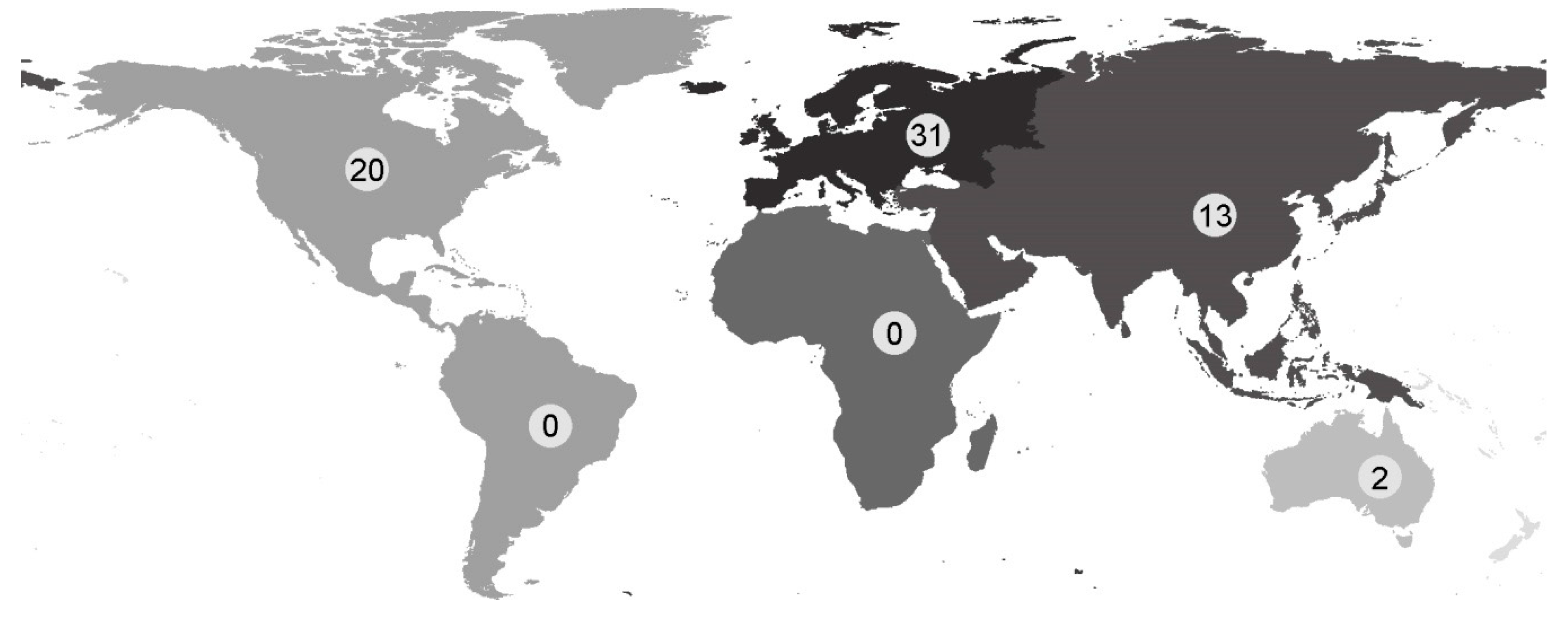
3.6. Geographical Framework

The database consists of 66 documents distributed geographically across the globe. As seen in Figure 5, there is a greater concentration in North America and Europe, as compared to the other continents (20 in North America, 31 in Europe, 13 in Asia, and 2 in Oceania).

Within the European continent, the 31 documents that examined the residential market were distributed as follows: 1 in Norway, 2 in Sweden, 1 in Denmark, 3 in Ireland, 3 in the United Kingdom, 2 in the Netherlands, 3 in Belgium, 3 in Germany, 4 in Switzerland, 2 in Italy, 2 in France, 1 in Portugal, and 4 in Spain.

In the American continent, the 20 documents examining the residential market are from North America and are distributed as follows: 17 in the United States (1 in Alaska, 2 in California, 1 in Colorado, 1 in Florida, 3 in Georgia, 3 in Oregon, 5 in Texas, and 1 that considers various studies) and 3 in Canada.

In Asia, they are distributed as follows: 4 in China, 6 in Japan, and 3 in the Republic of Singapore. In Oceania (Australia), there are 2 documents in Canberra.

3.7. Available Data

3.7.1. Analysis-1

In the first step, the documents comparing “labeled/non-labeled” with any qualification type were selected, in accordance with the classification of the data made in Section 3.5. The initial sample of 62 registers was used, made up of 19 registers having the ABCDEFG qualification and 43 registers with other qualification types (Figure 4). Then, the atypical uni-variate and multi-variate cases were eliminated (coded as A1*), using the following steps: (1) Those registers whose premium was more than three standard deviations (SD) apart were eliminated, discarding registers number 87 and 111; and (2) using the remaining registers, the regression model was calibrated and the Mahalanobis distance (DM) was calculated, eliminating those registers whose statistical significance was less than 0.001, as indicated by Hair et al. [92], excluding registers number 2, 3, 23, and 143. Thus, we obtained a final sample of 56 registers.

In

Table 2. Set of variables making up the study of analysis 1, with its units and description.

Category	Characteristics	Unit	Variable Description	Used
Financial characteristics (I)	Premium_EPC	numerical	Premium in the sales price of the housing (effect size: β)	Dependent variable
	SE	numerical	Standard error of the estimate	NO
	VAR	numerical	Variance of the estimate = SE2	Weighting variable
Characteristics of the publication (II)	Date_publication	numerical	Year of the document’s publication	YES
	Date_Before_Crisis	dummy	Indicates whether the data date is before, during or after the 2008 economic crisis	YES
	Date_During_Crisis	dummy
	Date_After_Crisis	dummy
	Num_Autor	numerical	Number of authors of the document	YES
	Journal_Article	dummy	Indicates if the document is a journal article or another type of document (report, congress, or thesis) 1 = Journal article; 0 = Other document	YES
	JCR	dummy	If the document is indexed in the Journal Citation Reports 1 = JCR; 0 = NO JCR	YES
	SJR	dummy	If the document is indexed in the Scimago Journal Rank 1 = SJR; 0 = NO SJR	YES
Continent (III)	America	dummy	Continent identifier: America, Asia, and Europe	NO
	Asia	dummy
	Europe	dummy
Construction type (IV)	Single_Family	dummy	Indicates if the document uses this type of data: Single family, multifamily, or multiple (combination of both)	NO
	Multifamily	dummy
	Multiple	dummy
Energy label (V)	Date_Label	numerical	Date of onset of energy label	YES
	Qualif_ABCDEFG	dummy	Indicates if the property has an ABCDEFG qualification = 1; or another qualification = 0 (CASBEE, Energy Star, LEED, Green, etc.)	YES
	Obligatory	dummy	Indicates if the label is mandatory (=1) or voluntary (=0)	NO
Model predictors (VI)	C_Dwelling	dummy	Indicates if any variable defining elements on the housing (surface area, number of baths or rooms, etc.) is included in the document	NO
	C_Building	dummy	Indicates if any variable defining building elements (existence of parking, elevator, swimming pool, garden, sporting areas, etc.) is included in the document	YES
	C_Neighborhood	dummy	Indicates if any variable defining the neighborhood where the housing is located (socio-economic level, type of residents, safety, etc.) is included in the document	YES
	C_Location	dummy	Indicates if any variable defining the location of the housing (residential area, distance to metro stops, etc.) is included in the document	YES
	C_Zone	dummy	Indicates if any variable defining the area or surroundings (density of the construction, types of activities, permitted land uses, etc.) is included in the document	YES
	C_Market	dummy	Indicates if any variable defining the real estate market (type of seller, time of sale on the market, etc.) is included in the document	YES
	C_Financing	dummy	Indicates if any variable defining the type of financing of the property, foreclosure, etc., are included	YES
Statistical data (VII)	Sample_size	numerical	Sample size used in the analyzed register	YES
	Data_web	dummy	Indicates if the sales prices have been obtained from a real estate portal (=1) or from another source (=0)	YES
	Price_area	dummy	Indicates if the dependent variable is introduced in the model as a price/surface area unitary value (=1) or not (=0)	YES
	R2fin	numerical	Determination coefficient of the analyzed register	NO
	f2	numerical	Statistical power of the analyzed register (see Equation (2))	NO
	t-test	numerical	Student’s t test	NO

, the 33 variables collected for this study were related, ordering them in seven categories. The unit with which each variable was measured was also indicated, along with a brief description of the same and whether or not it had been used in the final regression model.

Category I consists of the dependent variable, Premium_EPC, which contains the value of the variation in sales price of housing with an energy label, made up of the non-standardized β coefficients of the analyzed registers, all having a semi-logarithmic functional form. The second variable is the variance of the VAR estimation, calculated based on the squared standard error and used to attempt to resolve any potential publication bias, both in the meta-analysis or the meta-regression, according to [93].

Category II consists of eight variables, used to measure whether or not there is selection bias for the analyzed documents, based on the date of publication of the document, the period in which the data were collected, number of authors, type of document, and quality index of its indexing.

Category III consists of three dummy variables used to geographically locate the study data (America, Asia, and Europe).

Category IV consists of three dummy variables used to define the constructive typology. The registers are differentiated between one another if the sample consists of single family, multifamily, or multiple housing (when housing of both types are used in the register).

Category V consists of three variables used to define the data of the energy label used in the study, which are type of energy qualification used, date of onset of the label, and mandatory nature of the same.

Category VI consists of seven dummy variables used to identify whether or not certain predictor variables were used in the statistical model: The characteristics of the property, characteristics of the building, characteristics of the neighborhood, characteristics of the location, characteristics of the area, and characteristics of the market and of the financing.

Category VII consists of six variables that are used to define the statistical data of each analyzed register, such as: The origin of the prices (if coming from a real estate portal or not), whether or not the dependent variable is introduced in the model as a price/surface area, sample size, coefficient of determination of the model, and statistical power.

All of the dummy variables are coded with a value of 1 when they have said characteristics and a 0 when they do not. The descriptive statistics of all variables are shown in

Table 3. Descriptive statistics for the variables.

Category	Characteristics	Continuous Variables				Dummies Variables
		Mean	SD	Min.	Max.	Frec. (=1)	Percent (%)
Financial characteristics (I)	Premium_EPC	0.043406	0.039194	−0.056300	0.143000
	SE	0.010441	0.015311	0.000042	0.109095
	VAR	0.000339	0.001583	0.000000	0.011902
Characteristics of the publication (II)	Date_publication	2014.1	2.2	2007	2018
	Date_Before_Crisis					15	26.8
	Date_During_Crisis					8	14.3
	Date_After_Crisis					33	58.9
	Num_Autor	2.9	1.3	1	5
	Journal_Article					40	71.4
	JCR					27	48.2
	SJR					32	57.1
Continent (III)	America					27	48.2
	Asia					11	19.6
	Europe					18	32.2
Construction type (IV)	Single_Family					24	42.8
	Multifamily					17	30.4
	Multiple					15	26.8
Energy label (V)	Date_Label	2003.5	4.4	1991	2012
	Qualif_ABCDEFG					18	32.1
	Obligatory					25	44.6
Model predictors (VI)	C_Dwelling					56	100.0
	C_Building					18	32.1
	C_Neighborhood					5	8.9
	C_Location					40	71.4
	C_Zone					4	7.1
	C_Market					24	42.9
	C_Financing					4	7.1
Statistical data (VII)	Sample_size	85,632.2	300,537.3	125	1,609,879
	Data_web					12	21.4
	Price_area					18	32.1
	R2fin	0.8080	0.0799	0.5040	0.9040
	f2	5.0063	2.1899	1.0161	9.4167
	t-test	7.9288	6.9352	−1.1600	22.0200

Notes: Sample size 56; SD: Standard Deviation. Frec.: Frequency with value = 1.

.

Figure 6a shows the graphics of boxes created for each of the three continents based on the energy label. As seen, when other qualification types are used (LEED, BREEAM, etc.), atypical values appear in the Asian continent, with the American continent having the greatest dispersion and asymmetry, as compared to the average.

In Figure 6b, the mean of the percentage of the premium in the price for each of the continents is shown, with the percentage of the premium being lower with the ABCDEFG qualification. It is also found that in Europe, there is a mandatory label with the ABCDEFG qualification scale, while in America and Asia, there is greater diversity of non-mandatory labels.

3.7.2. Analysis-2

For this analysis, the registers with the ABCDEFG qualification were selected and the initial sample of 115 registers (Figure 4) was used. They were grouped together based on what the label analyzes: Labeled/non-labeled; grouped letters, ungrouped labels, and other non-comparable labels. Cases of labeled/non-labeled (19 registers) and non-comparable ones (5 registers) were discarded from this Analysis 2.

Next, abnormal cases were eliminated (A2* in Table 1), identifying registers from the same study that could be correlated: (1) Studies using different registers for the same type (isolated houses, semi-detached houses, etc.) in which case the register that includes the complete sample of cases of this type were selected, thereby eliminating registers 27–32, 75–79, and 99–104; and (2) studies that provide the premium value when offered and the premium once the property is sold; the latter is included, eliminating register 82. In this way, a final sample of 73 registers is obtained for Analysis 2.

3.8. Methodology

This document attempts to raise theoretical awareness regarding sales price premiums of residential housing containing an EPC, based on a systematic review using meta-analysis and meta-regression, with a descriptive, comparative, correlational, and exploratory design.

In this study, the work line of other authors was followed, analyzing the influence of the EPC on the price, using two distinct approaches: (1) Analysis-1 (A1): Quantifies the premium for the price of the housing having EPC as compared to those without it; (2) Analysis-2 (A2): Of the housing with an EPC, it quantifies the premium resulting from changing from one qualification to another within the analyzed scale. In this second way, it is only possible to analyze the ABCDEFG qualification, having observed that each author proposes distinct scenarios, considering different reference bases to measure the impact of the EPC on the price (see Section 3.8.2).

3.8.1. Analysis-1

Below, the steps followed to estimate the premium in the sales price of the housing with an EPC, as compared to housing without it, are described. First, a descriptive analysis is conducted and then, a study of publication heterogeneity and bias, a sensitivity analysis, and, finally, a meta-analysis and a meta-regression.

Heterogeneity in a meta-analysis can lead to distorted results. This heterogeneity may be due to: (1) Selection and publication biases; (2) a poor selection of the measurement of the effect; and (3) the different study results.

To avoid the selection and publication biases, documents published in distinct languages were selected, not only those in English. Moreover, in the meta-analysis, documents published in journals as well as other documents from the so-called grey literature were included (reports, congresses, and theses) as indicated by Begg [94]. Furthermore, the search for documentation was conducted in distinct databases and not only through the use of bibliographic references. To explore the existence of selection bias, a visual assessment was carried out with the funnel plot.

To avoid heterogeneity based on the selection of the type of measure to quantify the effect size, the selected documents are homogenous and comparable, since they all analyze the premium in the price of residential buildings that are commercialized for sale through HPM with semi-logarithmic estimates. A rigorous selection process was followed, eliminating extreme and atypical uni-variate and multi-variate cases, discarding the registers that were greater than three standard deviations and those whose statistical significance of the Mahalanobis distance was less than 0.001.

To evaluate and quantify the heterogeneity between the studies included in the analysis, three meta-analyses were carried out (by publication type, by data period, and by continent), as well as a meta-description with a meta-regression with randomized effects, comparing the distinct models and the X², Tau², and I² statistics. The statistical heterogeneity exists when the value of p is less than 0.05 for the X² statistic or the I² test is greater than 50%.

$$I^2=\frac{Q-\left(k-1\right)}{Q}x100,$$

(3)

where:

• Q is the test of the X² to assess the heterogeneity of the studies included in a meta-analysis, where the magnitude of the effect of each individual study is compared with the combined estimator;
• k − 1 are the degrees of freedom, where k is the number of studies.

The meta-regression analyses consider an initial model of fixed effects and a second model of random effects, as suggested in [12,95,96,97,98]. The fixed effects model assumes that there is no heterogeneity between the analyzed documents, such that all of these estimate the same effect and the differences are only due to chance [13,99].

$${\widehat{\theta }}_i=\theta +{\delta }_i,$$

(4)

where:

• ${\widehat{\theta }}_i$ is the dependent variable or the measurement of the effect (Premium_EPC), obtained from the results of the distinct registers analyzed, from i = 1, …, k;
• ${\delta }_i$ is the error committed in the observation i upon approaching $\theta$;
• $\theta$, is the fixed overall effect, which may be estimated with a weighted mean of the individual effects of each study:

$$\theta =\frac{{{\displaystyle \sum }}_{i=1}^k{w}_i{\widehat{\theta }}_i}{{{\displaystyle \sum }}_{i=1}^k{w}_i},$$

(5)

where:

• $w_i$ are the weights or weighting carried out by the inverse variance method ($w_i=\frac{1}{{\sigma }_i^2})$;
• ${\sigma }_i^2$ is the variance of each estimator of the meta-sample.

The random effects model assumes that there is heterogeneity in the analyzed documents, such that, in addition to the overall effect and the estimation error, the random effect generated from each study is considered [13,99]. The random effects model regards the studies as a sample of a larger universe of studies and can be used to infer what would likely happen if a new study were performed.

$${\widehat{\theta }}_i=\theta +{\theta }_i+{\delta }_i,$$

(6)

where:

• ${\widehat{\theta }}_i$ is the dependent variable or measurement of the effect (Premium_EPC), obtained from the results of the distinct registers analyzed, from i = 1, …, k;
• ${\theta }_i$ is the effect to estimate in the ith study of the meta-sample;
• ${\delta }_i$ is the error committed in the observation i upon approaching $\theta$;
• $\theta$ is the fixed overall effect that can be estimated as a weighted mean of the individual effects of each study:

$$\theta =\frac{{{\displaystyle \sum }}_{i=1}^k{w}_i{\widehat{\theta }}_i}{{{\displaystyle \sum }}_{i=1}^k{w}_i},$$

(7)

where:

• w_i is the weight associated with each estimator of the sample ($w_i=\frac{1}{{\sigma }_i^2+{\tau }^2}$);
• ${\sigma }_i^2$ is the variance of each estimator of the meta-sample;
• ${\tau }^2$ is the variance between studies.

Different methodologies may be used to calculate the overall effect, based on the dependent variable and the characteristics to be analyzed [100]. There are various estimators to calculate the variance between studies (${\tau }^2$) such as the DerSimonian and Laird [101] (DL), Hunter and Schmidt (HS), Hedges and Olkin [11] (HO), maximum likelihood (ML), and restricted maximum likelihood (REML), among others. According to Viechtbauer [102], when it comes to selecting one of these methods, the objective is to optimize: (1) The bias (difference between the estimated value and the actual value); (2) efficiency (should not be affected by sampling fluctuation); and (3) the mean square error (MSE). Veroniki et al. [103] conducted another study in which a larger number of estimators was analyzed and they concluded that the selection of the most appropriate estimator depends on: (1) If a zero value of the variance is considered possible; (2) properties of the estimators for the bias and efficiency, which depends on the number of studies included and the real variance; and (3) ease of application.

The meta-regression is performed with the six estimators shown in

Table 4. Summary of the most noteworthy characteristics when selecting an estimator for a random model.

Method	Estimator	Considerations
Method of moments estimators	DerSimonian and Laird (DL)	It is acceptable when the real levels of the variance between studies is small or almost zero, but when the variance is large, the DL estimator may produce estimates having significant negative bias.
	Hedges and Olkin (HO)	The HO functions well in the presence of substantial variation between studies, especially when the number of studies is large (that is, k ≥ 30), but produces a large MSE. In general, it produces estimates that are slightly greater than those produced in the DL and REML methods.
	Hunter and Schmidt (HS)	If the sample is negatively or positively biased, it leads to an under-estimation or over-estimation of the real variation between studies. When the sample size is small, an under-estimation may be produced in the heterogeneity.
Maximum likelihood estimators	Maximum likelihood (ML)	This is an asymptotically efficient method that requires an iterative solution; thus, it depends on the selection of the maximization method. In addition, it has the smallest MSE in comparison with the REML and HO methods, but the greatest quantity of negative bias between them.
	Restricted maximum likelihood (REML)	It may be used to correct the negative bias associated with the ML method. It is not adequate when there are few observations. It has less bias with dichotomous data than the ML, but has a greater MSE. For continuous data, REML is the preferred approach when large studies are included in the meta-analysis.
Bayes estimators	Bayes estimators (Bayes)	It is recommended when there are samples with less than 5 observations, since less bias is generated as compared to other stimulators (DL, HO, or REML).

Note: Author’s own creation based on Veroniki et al. [103].

. In addition, the following hypotheses are verified: (1) Normality of the distribution of the dependent variable with the Kolmogorov–Smirnov test, a frequency diagram, and a graph of normality residuals; and (2) homoscedasticity, using the Breusch–Pagan test.

The calculations were made with a 95% confidence level. For these analyses, OpenMEE [104] software was used, as well as the R “metafor” package (version 2.0) [105] and the IBM SPSS Statistic (version 21) and the SPSS macros by Ahmad Daryanto for the Breusch–Pagan and Koenker test (July 2018) [106].

3.8.2. Analysis-2

For the registers of the ABCDEFG qualifications, the steps followed to quantify the premium resulting when changing from one level to another in the qualification scale were carried out via descriptive analysis of the registers, based on the reference base used by the authors for each document: (1) Groupings of letters (for example: DEFG compared to ABC or EFG compared to ABCD); (2) independent letters, using one letter as a reference (D, F, or G) and analyzing the price premium in comparison to other individual or grouped letters (AB, EFG, or FG); and (3) housing without qualification (NT) and analyzing the price premium in each of the qualification letters individually or grouped (AB and CDEFG).

4. Results

4.1. Analysis-1: Analysis of the Impact on Prices of Housing with an EPC as Compared to Housing without Qualifications

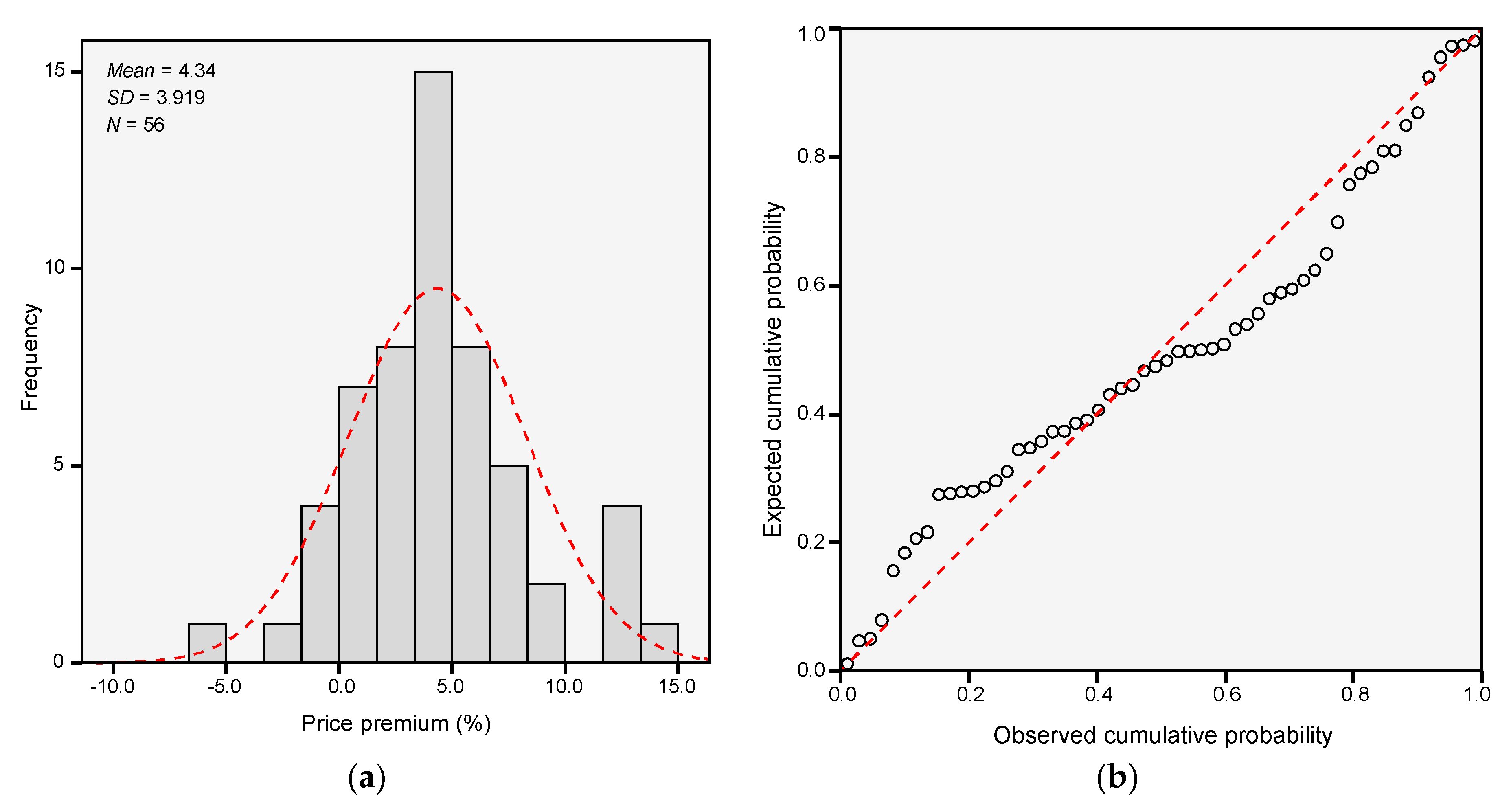
4.1.1. Normality and Heteroscedasticity

The normality of the distribution of the dependent variable (Premium_EPC) has been verified with the Kolmogorov–Smirnov test, which was found to be not statistically significant (D = 0.086, p = 0.200, n = 56), suggesting that the sample follows a normal distribution, as represented in the histogram (Figure 7a) and a normal probability plot of the standardized residual (Figure 7b). To evaluate the existence of heteroscedasticity, the Breusch–Pagan test was conducted (BP = 19.77, df = 15, p = 0.181), with the results suggesting that the null hypothesis of heteroscedasticity should not be rejected; thus, heteroscedasticity was not found.

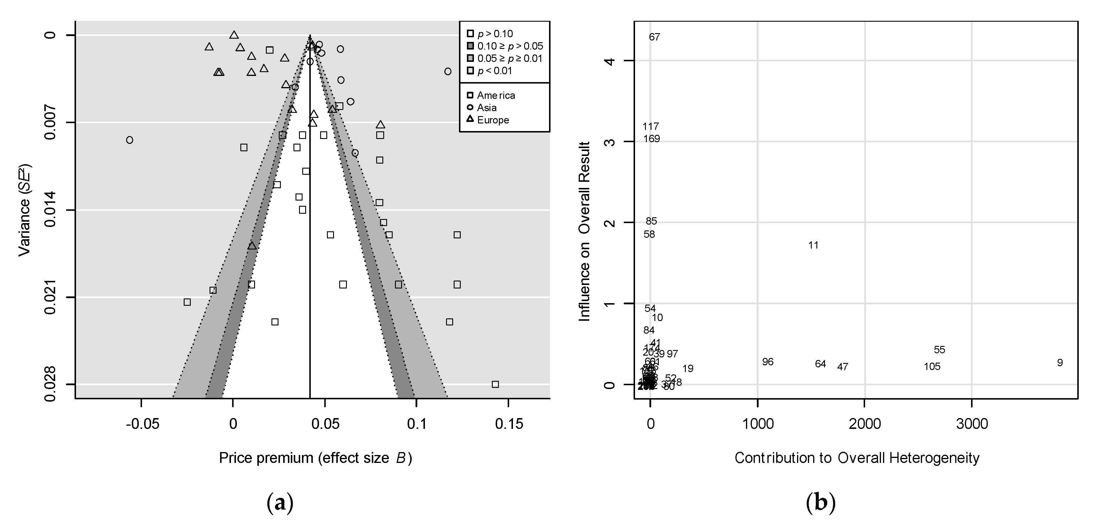
4.1.2. Heterogeneity and Publication Bias

Cochran’s Q test for the model of fixed effects was found to be statistically significant (Q = 17821.36, df = 55, p < 0.0001), confirming the existence of heterogeneity for the sample. In order to determine the origin of the heterogeneity, a funnel plot and Baujat plot were used.

To evaluate publication bias, a visual assessment was conducted with the contour-enhanced funnel plot [107], introducing the studies grouped together by continent and shadowing the regions based on their significance level (Figure 8a). It was observed that a major asymmetry exists in the documents, concentrated in the upper left-hand area of the graph (mainly European studies). This is the area where the results have a greater precision, with smaller confidence intervals and greater statistical significance. A certain accumulation was seen in the observations corresponding to America, which have a greater dispersion of the variance and are distanced from the observations of Europe and Asia. This suggests that the heterogeneity is not due to selection bias, but rather, to the localization factor.

The X axis of Baujat et al. [108] (Figure 8b) reveals the contribution of each study to the overall heterogeneity of the sample (through the Cochran Q test), while the Y axis represents the influence of the study on the overall results. Tests with greater heterogeneity and a larger influence appear in the upper right-hand area of the graph (register 11). Those that contribute more to the heterogeneity are situated in the lower right-hand area of the graph (registers 9, 47, 55, 64, 96, and 105), and those situated in the upper left-hand region reveal a greater influence (registers: 58, 67, 85, 117, and 169). As a sensitivity analysis, upon eliminating these 12 registers, approximately 87.36% of the heterogeneity is removed (Q = 2251.97, df = 43, p < 0.0001), but it continues to be statistically significant, suggesting that it would be necessary to continue eliminating registers. If repeating the process two more times, the remaining sample would have 21 observations, reducing the heterogeneity by approximately 99.19%, but not fully eliminating it (Q = 144.31, df = 20, p < 0.0001). These results suggest that even upon eliminating over half of the registers, the heterogeneity remains, and therefore, it is considered that this heterogeneity is not the result of publication bias, but rather, it is a result of the very data that are being analyzed [109].

4.1.3. Sensitivity Analysis

Figure 9 offers a sensitivity analysis based on a forest plot in which the influence of each of the studies on the overall effect is examined. The graph represents the overall combined effect of the sales premium of the housing that has EPC, every time one of the studies is omitted. The results show that when some of the included studies are omitted, neither the direction nor the significance are changed, upon comparing these with the combined estimate from all of the studies (overall effect = 0.0420). There is also no evidence of a significant change in the heterogeneity index (I²), whose values are between 99.6% and 99.8%; therefore, it may be said that none of the studies notably affects the overall estimated result, and therefore, the results may be considered robust [110] and [111].

However, it may be useful to highlight the influence of two studies: Addae-Dapaah and Chieh [51] and Yoshida and Sugiura [41] which are found to fall outside of the 95% confidence interval of the overall effect of all of the studies (IC–95% = 0.0407, 0.0433), which, upon being eliminated, produce a reduction or increase in the estimate of the overall combined effect.

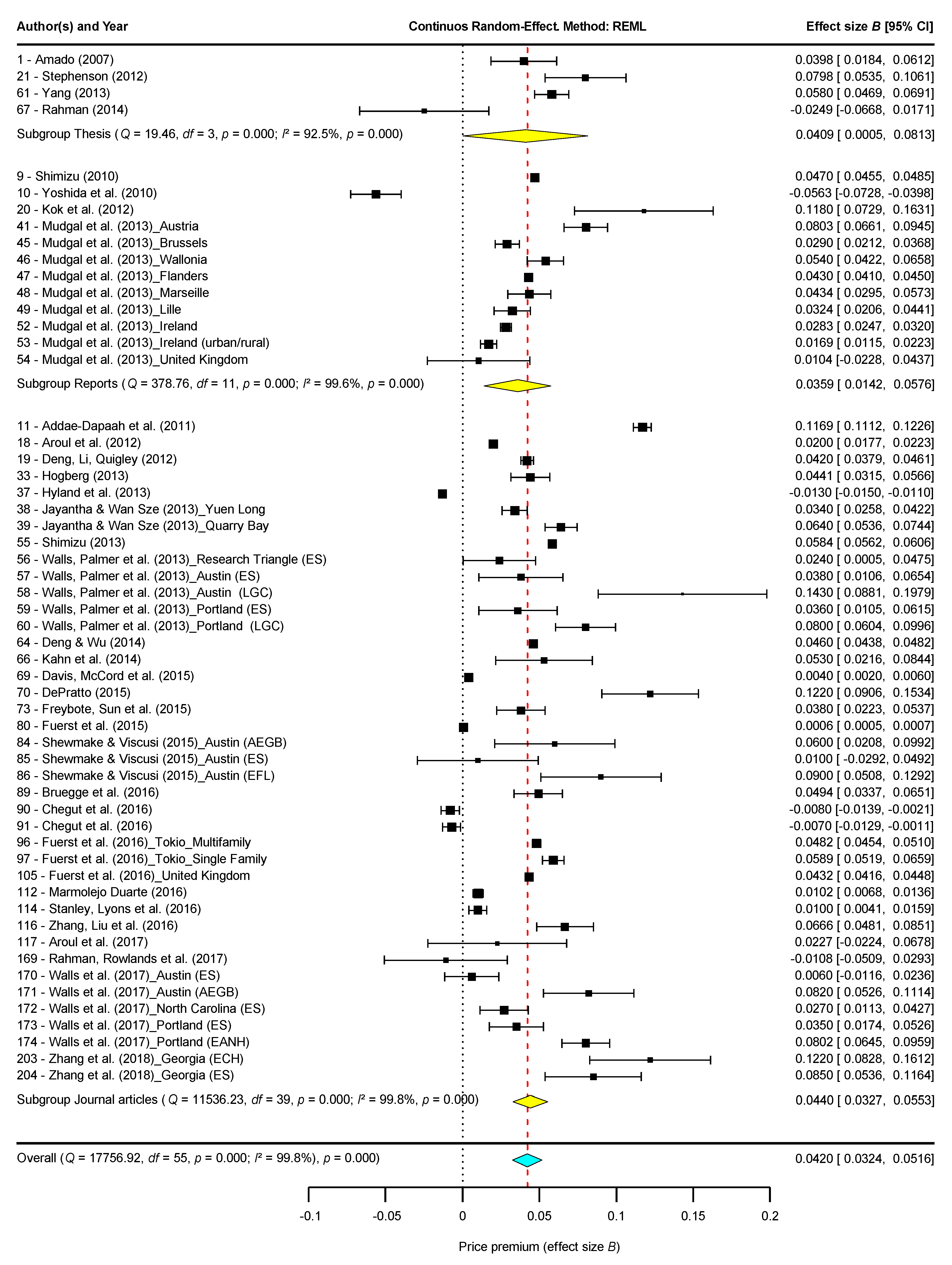
4.1.4. Meta-Analysis

Since the fixed effects and random effects methods are exclusive, one of these should be selected based on the heterogeneity (Q test) [97]. As shown in the previous section, heterogeneity exists. Therefore, three meta-analyses were conducted, forming sub-groups [112], based on the publication type (Figure 10), based on the data period (Figure 11) and based on the continent (Figure 12), in order to verify whether or not the heterogeneity of the registers is a result of these factors, estimating the effect for each sub-group with a random effects model through a forest plot. To create this model, distinct estimators may be used, but for the estimate of the confidence interval for the variance between studies, Veroniki et al. [103] consider that better results are obtained with a REML estimate, as compared to the DL estimate. Therefore, this was the one used in this study.

Various forest plots appear in the document. As clarifying notes for all of these, we should note: (1) To identify the studies with more than one register, in addition to indicating the «register» and the «author (year)», the «location (label)» was included; and (2) for interpretation purposes, “■” indicates the study results and the size is proportional to the contribution of the register to the overall result. The horizontal lines, “―”, correspond to the confidence intervals and reveal the precision of the studies and whether or not they are statistically significant (when they do not cross the black dotted line that corresponds to a null effect, zero). 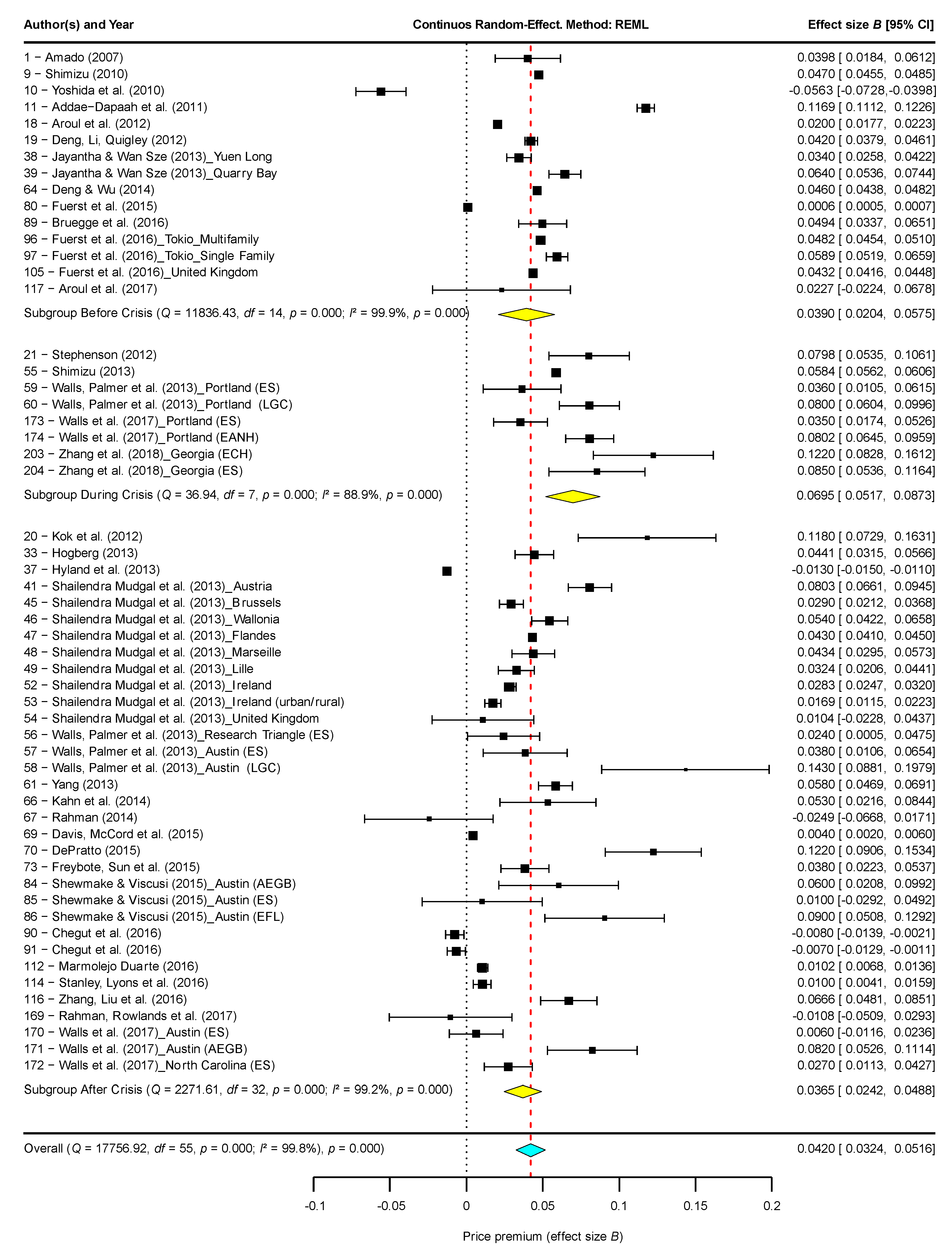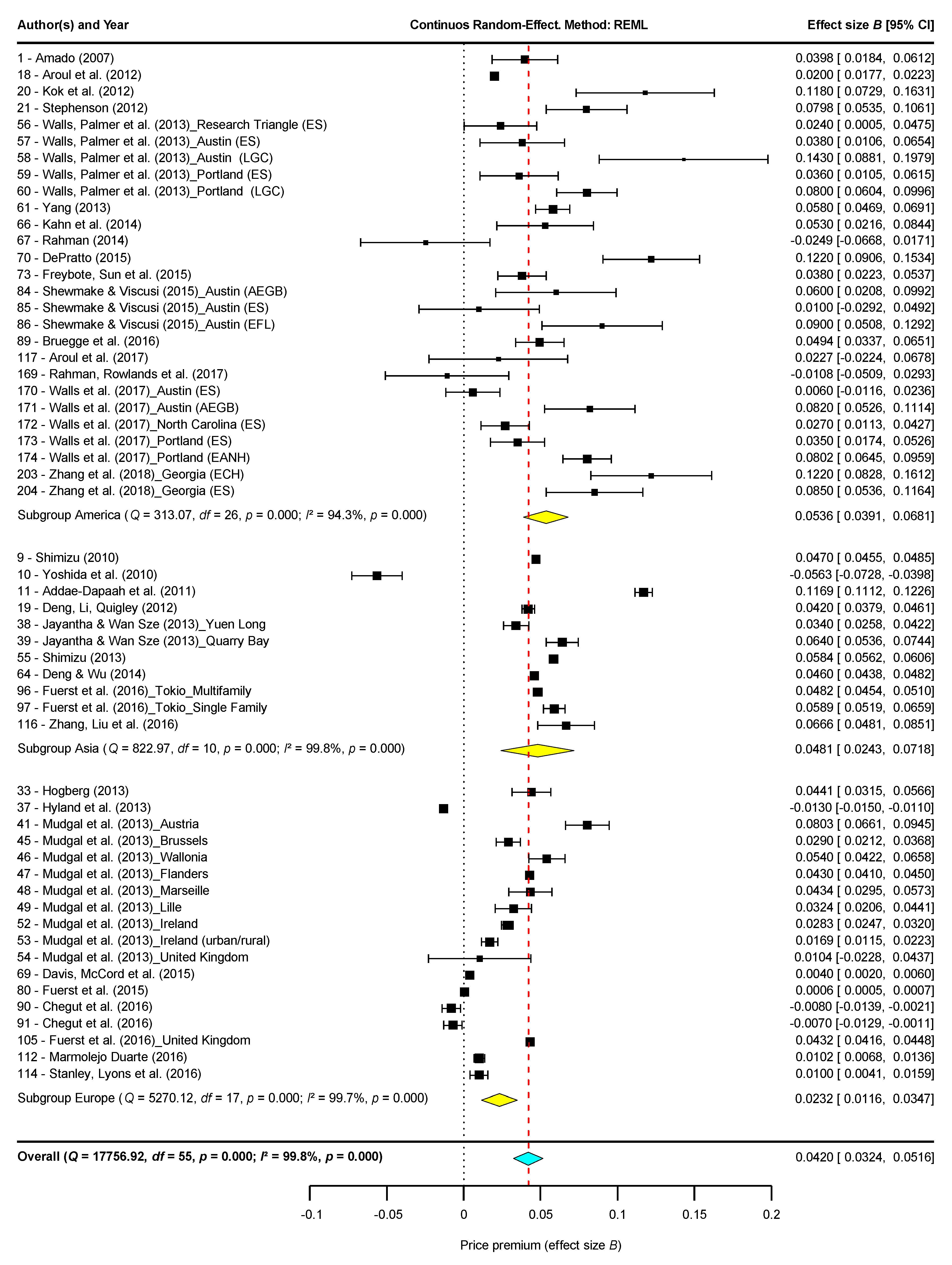“ ” Result of the combined effect, by sub-groups (type of study, data period or continents) and “ ” result of the overall combined effect, both are to be interpreted as the weighted average effect or “combined” effect size, obtained according to Equations (6) and (7). “¦” Red dashed line that represents the value of the overall combined effect.

In Figure 10, it is found that a price premium is generated for the housing sales with an overall combined effect of 4.20%. However, when the publication sub-group considered is the Master’s thesis, it is 4.09%. If reports are considered, it is 3.59% and if journal articles are looked at, it is 4.40%. These are all statistically significant values. In the thesis sub-group, it is observed that the four registers are distributed across both sides of the line that defines the overall combined effect. Thus, the sub-sample would be homogenous with regards to selection bias. On the other hand, the confidence intervals of the registers are quite broad, suggesting a greater dispersion in the premiums. There are 12 publications in the reports sub-group, while the registers have more concentrated confidence intervals as compared to in the journal articles. The journal articles sub-group has 40 registers, revealing more diverse confidence intervals than in the previous sub-groups.

It is found that the three publication types have superimposed results (yellow diamonds), so, apparently, there is no significant difference between the average effects of the sub-groups and the overall combined effect. Therefore, it cannot be affirmed that the heterogeneity of the registers is a result of the type of publication considered.

In Figure 11, the studies are organized into three sub-groups according to the date of data collection: The first group, mainly compiled before 2008, shows an effect size of 3.90%; the second group, gathered from 2006–2010, shows an effect of 6.95%; and, finally, the third group of data mainly collected after 2008, shows an effect of 3.65%. The resulting analysis indicates similar effects in the first and third sub-groups, both remaining close to the value of the overall combined effect. By comparison, the second sub-group corresponding to the crisis period shows a greater impact of the energy qualification on price increase than the other two sub-groups. Apart from the date time slot, this disparity is also justified by the predominant house typology. Most of the studies in the second sub-group are based on cases located in America, where single family dwellings are the predominant kind.

In Figure 12, the sub-groups were analyzed by continent, with an effect of 5.36% in America, 4.81% in Asia, and 2.32% in Europe. All of these values are statistically significant. In America, it is observed that the 27 registers are distributed across both sides of the line defining the overall combined effect. Therefore, the sample will be homogenous in this subset with regards to selection bias. On the other hand, the confidence intervals of the registers are, generally speaking, quite broad, suggesting a greater dispersion in the premiums. In Asia, the number of registers is 11, less than half of those in America. However, the registers have smaller confidence intervals and there is not as much dispersion in the premiums. In Europe, there are 18 registers of which only one has broad confidence intervals, and within this sample there is not much dispersion.

It is found that the results for America and Asia are relatively well aligned with one another (yellow diamonds), so apparently, there is no significant difference between them. On the other hand, when comparing these two continents with Europe, it may be seen that the premium is approximately half of that of America and Asia. The confidence intervals of America and Europe do not even overlap (width of the yellow diamonds). Thus, there is a significant difference between the average values. This difference may result in the heterogeneity that was observed in the previous section.

What factors cause these differences? First, in Europe, the energy label is mandatory, which is not the case in either America or Asia. Second, the energy label in Europe (the ABCDEFG qualification) does not precisely quantify like the other labels. Furthermore, the construction type may also affect the results. An attempt is made to resolve these issues by proposing a graphic analysis (Figure 13) and a meta-regression (Section 4.1.5), which reveals the multi-collinearity existing between the continents, construction type, and energy labeling type.

4.1.5. Meta-Regression

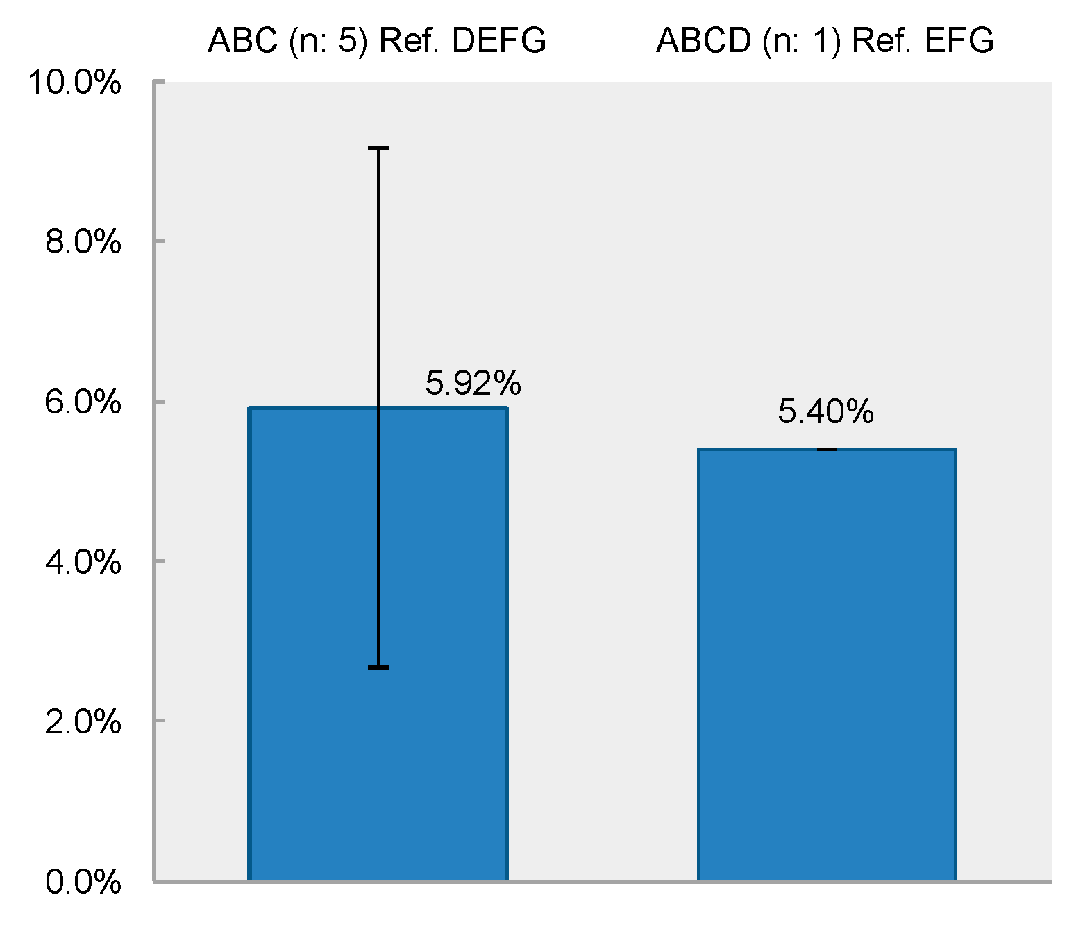
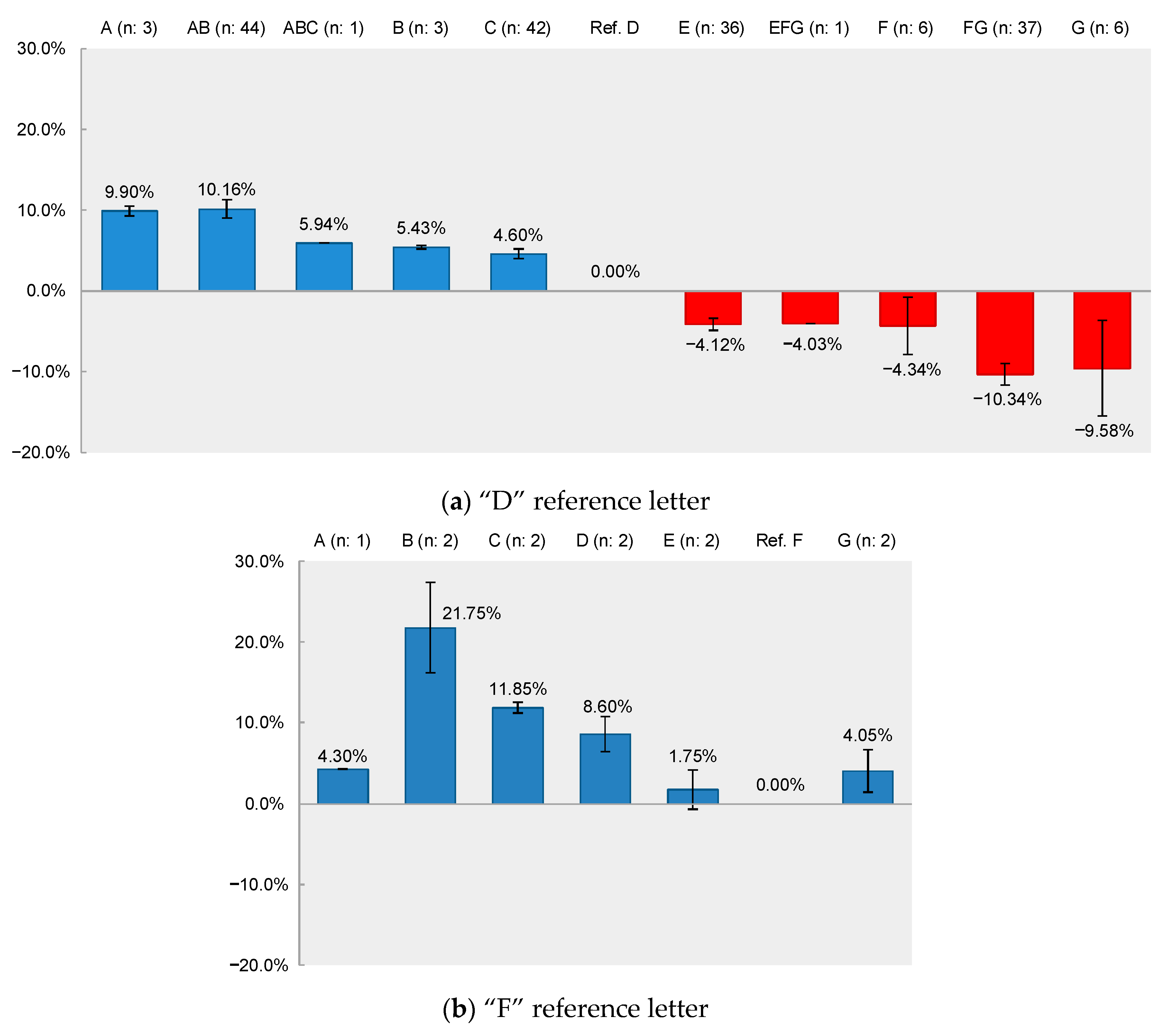
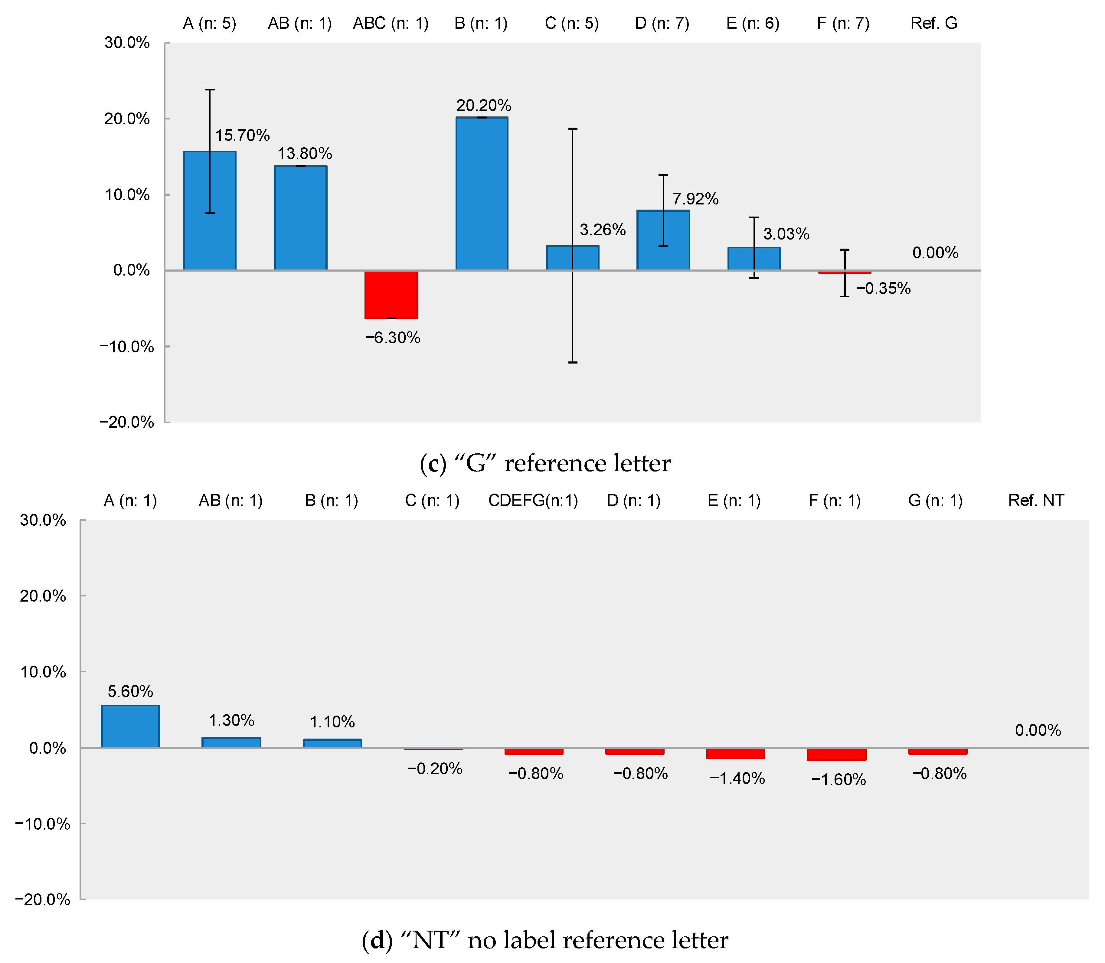
The object of this subsection is to determine whether or not the heterogeneity existing between the registers is related to the specific characteristics of these documents [112]. Of the variables described in Table 2, those having problems of multi-collinearity with other variables have been discarded, as is the case of the continent with construction type and energy labeling, or the coefficient of determination with the statistical power. Furthermore, those variables in which no variability existed in the classification were eliminated, as was the case for the housing characteristics (C_Dwelling) or when the number of observations is low (Sample_size). In all, 13 variables were discarded: SE, America, Asia, Europe, Single_Family, Multifamily, Multiple, Obligatory, C_Dwelling, R²fin, f², and t-test.

Since the existence of heterogeneity has been found in the sample, the use of fixed effects for the meta-regression was discarded. A random effects model was created using distinct methods (

Table 5. Meta-regression with random effects.

Category	Characteristics		DL	HO	HS	ML	REML	Bayes
	(Constant)	B	−18.582 **	−19.006 *	−14.976 ***	−18.718 **	−18.967 *	−18.987 *
		SE	6.409	9.259	1.012	7.033	8.834	9.049
		Z	−2.899	2.053	−14.792	−2.661	−2.147	−2.098
Characteristics of the publication (II)	Date_publication	B	0.006 *	0.005	0.007 ***	0.006	0.005	0.005
		SE	0.003	0.004	0.000	0.003	0.004	0.004
		Z	2.129	1.442	16.712	1.929	1.515	1.477
	Date_Before_Crisis	B	−0.013	−0.014	−0.008 *	−0.013	−0.014	−0.014
		SE	0.013	0.018	0.004	0.014	0.017	0.018
		Z	−1.033	−0.760	−2.201	−0.958	−0.792	−0.775
	Date_After_Crisis	B	−0.002	0.001	−0.033 ***	−0.001	0.000	0.001
		SE	0.012	0.017	0.004	0.013	0.016	0.017
		Z	−0.173	0.047	−7.471	−0.095	0.030	0.039
	Num_Autor	B	0.010 *	0.010	0.002	0.010 *	0.010	0.010
		SE	0.004	0.006	0.001	0.004	0.006	0.006
		Z	2.427	1.793	1.891	2.254	1.867	1.829
	Journal_Article	B	0.023	0.023	0.049 ***	0.023	0.023	0.023
		SE	0.016	0.022	0.004	0.017	0.021	0.022
		Z	1.501	1.036	13.834	1.362	1.085	1.060
	JCR	B	−0.022	−0.019	−0.024 ***	−0.021	−0.019	−0.019
		SE	0.015	0.021	0.003	0.016	0.020	0.021
		Z	−1.437	−0.883	−7.820	−1.264	−0.937	−0.909
	SJR	B	−0.035 *	−0.037	−0.065 ***	−0.035 *	−0.037	−0.037
		SE	0.016	0.023	0.004	0.018	0.022	0.022
		Z	−2.154	−1.608	−16.138	2.006	−1.672	−1.639
Energy label (V)	Date_Label	B	0.004 **	0.004 *	0.000	0.004 **	0.004 *	0.004 *
		SE	0.001	0.002	0.000	0.001	0.002	0.002
		Z	2.988	2.352	0.973	2.833	2.434	2.392
	Qualif_ABCDEFG	B	−0.054 ***	−0.054 **	−0.038 ***	−0.054 ***	−0.054 **	−0.054 **
		SE	0.015	0.021	0.003	0.016	0.020	0.021
		Z	−3.665	−2.580	−12.207	−3.354	−2.698	−2.637
Model predictors (VI)	C_Building	B	−0.000	−0.000	−0.004 *	−0.000	−0.000	−0.000
		SE	0.010	0.015	0.002	0.011	0.014	0.015
		Z	−0.032	−0.024	−2.291	−0.030	−0.025	−0.024
	C_Neighborhood	B	0.022	0.023	−0.005	0.023	0.023	0.023
		SE	0.015	0.021	0.005	0.016	0.020	0.020
		Z	1.504	1.115	−0.975	1.400	1.161	1.137
	C_Location	B	−0.023 *	−0.023	−0.014 ***	−0.023 *	−0.023	−0.023
		SE	0.010	0.014	0.002	0.011	0.014	0.014
		Z	−2.380	−1.604	−8.772	−2.154	−1.687	−1.644
	C_Zone	B	0.022	0.022	0.020 ***	0.022	0.022	0.022
		SE	0.017	0.025	0.004	0.019	0.024	0.024
		Z	1.276	0.876	5.034	1.160	0.919	0.897
	C_Market	B	0.032 **	0.033 *	0.020 ***	0.032 **	0.033 *	0.033 *
		SE	0.011	0.016	0.003	0.012	0.015	0.016
		Z	2.926	2.051	7.993	2.676	2.146	2.097
	C_Financing	B	−0.045 *	−0.048	−0.009	−0.046 *	−0.048	−0.048
		SE	0.019	0.026	0.011	0.021	0.025	0.026
		Z	−2.341	−1.843	−0.805	−2.220	−1.908	−1.875
Statistical data (VII)	Sample_size	B	0.000 *	0.000	−0.000 ***	0.000	0.000	0.000
		SE	0.000	0.000	0.000	0.000	0.000	0.000
		Z	2.055	1.585	−9.966	1.936	1.644	1.614
	Data_web	B	−0.004	−0.008	0.018 ***	−0.005	−0.008	−0.008
		SE	0.010	0.015	0.002	0.011	0.014	0.014
		Z	−0.388	−0.541	7.745	−0.461	−0.538	−0.540
	Price_area	B	−0.016	−0.018	0.009 ***	−0.017	−0.018	−0.018
		SE	0.013	0.019	0.002	0.015	0.018	0.019
		Z	−1.212	−0.941	3.994	−1.146	−0.976	−0.958
Mixed-Effects Model	Tau2:		0.000 (0.000)	0.001 (0.000)	0.000 (0.000)	0.001 (0.000)	0.001 (0.000)	0.001 (0.000)
	I2:		96.24%	98.34%	8.97%	96.95%	98.16%	98.25%
	H2:		26.63	60.07	1.10	32.80	54.25	57.15
	R2:		47.79%	29.93%	94.75%	55.75%	27.51%	28.48%

Notes: Sample size 56. B: Meta-regression coefficient; SE: Standard Error; Z value, signification: ***: 0.001; **: 0.01; *: 0.05. Tau²: Estimated amount of residual heterogeneity; I²: Residual heterogeneity/unaccounted variability; H²: Unaccounted variability/sampling variability; R²: Amount of heterogeneity accounted. DL: DerSimonian and Laird, HO: Hedges and Olkin, HS: Hunter and Schmidt, ML: Maximum likelihood, REML Restricted maximum likelihood, and Bayes: Bayes estimators (see Table 4).

): DL, HO, HS, ML, REML, and Bayes. It is observed that since the sample is positively biased, the HS method offers an over-estimation of the variance, resulting in almost all of the characteristics being significant at p < 0.001 and the determination coefficient being very high (94.75%). Of the other methods, the HO, REML, and Bayes offered similar results, with 17 of the 18 variables obtaining the same value of B and with very little variation in the coefficient of determination (2.42%). Therefore, either of these would be appropriate. For this document, the REML method was selected, in line with [102,103,104,105,106,107,108,109,110,111,112,113,114], given that, according to these authors, it is the method that offers the best results in terms of bias and efficiency as compared to the DL, ML, HS, and HO methods.

The results of the REML model reveal that, with respect to the publication characteristics (category II), the housing price premium is greater in documents having a more recent publication date (Date_publication = 0.005, not significant), in documents with a larger number of authors (Num_Autor = 0.010, not significant) or if the document is a journal article (Journal_Article = 0.023, not significant). On the other hand, the premium decreases when the data in the documents are prior to the 2008 crisis (Date_Before_Crisis = −0.014, not significant) and if the published document has some sort of JCR quality index (−0.019, not significant) and/or SJR (−0.037, not significant). If the data in the documents are post-crisis, the price remains stable with respect to the period during the crisis (Date_After_Crisis = 0.000, not significant).

When analyzing the characteristics of the energy label (category V), it is observed that the premium is lower when the ABCDEFG label is used (Qualif_ABCDEFG = −0.054, significant), as compared to the other label types (LEED, Energy Star, etc.). On the other hand, the premium increases when the start date of the qualification is more recent (Date_Label = 0.004, significant).

Within category VI of the model predictor variables, the premium decreases when characteristics defining the building are not used (C_Building = −0.000, not significant) such as elevator, swimming pool, garden or garage, etc.; the property location (C_Location = −0.023, not significant) or the financing (C_Financing = −0.048, not significant). On the other hand, it increases when using neighborhood characteristics (C_Neighborhood = 0.023, not significant) such as delinquency rate, neighborhood income, or percentage of elderly individuals; characteristics of the area (C_Zone = 0.022, not significant) such as density of construction or land use; and market characteristics (C_Market = 0.033, significant) such as commercialization type or time of sale.

Finally, the statistical data VII category is positively affected by the number of register observations (Sample_size = 0.000, not significant), but the premium decreases when the economic data is obtained from web pages (Data_web = −0.008, not significant) or if the sales price has been introduced in the model as a monetary unit divided by the surface area (Price_area = −0.018, not significant).

4.2. Analysis-2

In this second analysis, the housing having EPC with the ABCDEFG qualification are examined, and the premium resulting from changing from one value to another within the analyzed qualification scale was quantified. This type of analysis has an advantage over the previous type, since it permits the identification of whether the housing with high qualifications have higher price premiums than those with low qualifications. One problem found in this research is that the reference base used by the distinct authors varies, and therefore, there are few cases that can be compared, to thereby quantify these values.

Of the registers included in Table 1, the sales price premiums of the EU’s EPC having the “ABCDEFG qualification” were analyzed for two reasons: (1) This qualification is mandatory in EU member countries; (2) it permits the quantification of the premium that passes from one value to another within the qualification scale; and (3) there is a large number of registers with this qualification (73 registers).

The registers analyzed are classified based on the reference base and these are: (1) Letter groupings: DEFG compared to ABC or EFG compared to ABCD (Figure 14); and (2) independent letters: Using as a reference the letter D, F, G, or NT (no label) and analyzing the price premium generated from one housing property to another with a distinct qualification, be they individual (A, B, C, D, E, F, or G) or grouped letters (AB, ABC, EFG, or FG), see Figure 15.

In Figure 14, when using the letter groupings as a reference, the most efficient energy letter qualifications ABC and ABCD have a price premium that is 5.92% and 5.40%, respectively, as compared to the less efficient groupings (DEFG and EFG).

When using the letter D as a reference (Figure 15a), the results are as expected: An increase in price premium as a result of a better energy qualification. That is, for two homes with equal conditions, one having a D qualification and the other with an A qualification, the latter will have a 9.90% higher sales price.

On the other hand, when graphically analyzing the sales premiums using the letter F as the reference (Figure 15b), certain incoherencies are observed. Housing with lower qualifications (G) have an increase in sales price of 4.05%, similar to those of the properties with A qualifications, and greater than those having an E or F qualification. This trend continues to appear when the reference qualification is the letter G (Figure 15c), where the housing qualified with a letter C and E have similar premiums at 3.26% and 3.03%, respectively, but housing with a grouped ABC qualification had a negative premium of 6.3%, suggesting that houses with the lowest qualification (G) were valued higher. Finally, if the reference is non-qualified properties (Figure 15d), only housing with very high qualifications (A, B, or AB) were found to have positive premiums, with the rest having negative premiums.

5. Discussion

5.1. Analysis-1

If collating the results obtained in the model of housing with an EPC as compared to housing that is not qualified, it is observed that in Europe (where energy qualification is mandatory), there are more homogenous price premiums, with these results being in line with other studies [25,26,34,35,36,75]. However, in America, due to the greater number of labels, there is also a greater variability in the results, obtaining a range that is between −2.49% and 14.3%. The lowest values are those of [32,67,87], while the highest are [38,55,62,69]. To avoid this variability, it is recommended that mandatory labels be used in both America and Asia, as suggested by Fizaine et al. [22]. Ankamah-Yeboah and Rehdanz [19] believe that greater premiums are obtained in the voluntary labels, since they consider that these are more highly valued than the mandatory ones, but they advocate policies that implement mandatory labeling, since it is understood that voluntary labeling tends to lose value over time.

If comparing the overall combined effect (4.20%) obtained in this document with similar studies, it is found that the first meta-analysis in 2014 obtained a premium of 7.6% [19], and the second in 2016 obtained 4.3% [20], while the third in 2018 had a range of values from 3.5–4.5% [22]. It is observed that the premium obtained in this study is coherent with other studies and the mean effect of the premium has stabilized.

For the meta-regression, the option adopted with the REML estimator is considered valid (in accordance with the cited literature) although its explanatory power is low at 27.51%. The proposed model cannot explain all of the variation existing in the data, as noted by Nelson and Kennedy [115].

Another problem found in this research is the lack of data in the existing studies, which complicates and restricts the use of the meta-analysis, as indicated by authors such as [22] and [115].

5.2. Analysis-2

As for the results to quantify the premium, which means changing from one value to another within the ABCDEFG qualification scale, a unique value may not be given, since the data available are based on distinct scenarios and distinct reference bases have been used to measure the impact on the EPC price. The results are heterogeneous and do not include sufficient information to offer conclusive results. Although a specific value cannot be given, there is a clear trend for the high qualifications (A, B, or C) to have greater price premiums. Even with a reduced sample, the graphs appear to reveal that the absence of information in the energy label favors sale of housing with poorer qualifications, as suggested by Marmolejo Duarte [78] in Spain.

Therefore, it is recommended that in future studies, qualification letter groupings should not be used and the reference qualification should always be the same (recommending the letter D), as suggested by Fizaine et al. [22].

6. Conclusions

This study analyzed two issues: (1) Analysis-1 (A1): Quantify the price premium of housing with an EPC as compared to those without this qualification; and (2) Analysis-2 (A2): In housing having an EPC, quantify the premium resulting from changing from one qualification to another, within the analyzed scale.

Having completed a thorough literature review from recent years, including 96 documents, certain criteria were adopted for admission of these documents, classifying the data based on analysis type to be carried out, eliminating abnormal data and obtaining a final sample of 66 documents forming a total of 58 and 73 registers for Analysis-1 and Analysis-2, respectively.

For Analysis-1, descriptive statistics were used, comparing the normality and homoscedasticity of the registers. To avoid publication bias, documents were collected from diverse sources. To evaluate whether or not the final sample was heterogeneous and if there was publication bias, an improved funnel plot was created, along with a Baujat plot and a sensitivity analysis, and thus permitting to identify that heterogeneity results from the same data, which is corroborated via three meta-analyses (by publication type, by data period, and continent) and a meta-regression.

In Analysis-2, bar graphs were made with the mean of the values registered based on the analyzed classification and the reference classification. The heterogeneity in the reference letter used by distinct studies hinders their comparison.

Based on all of the analyses carried out, the following conclusions may be reached:

• Housing with an EPC has an overall combined effect on the sales price premium of 4.20% more than housing of similar characteristics that does not have this qualification;
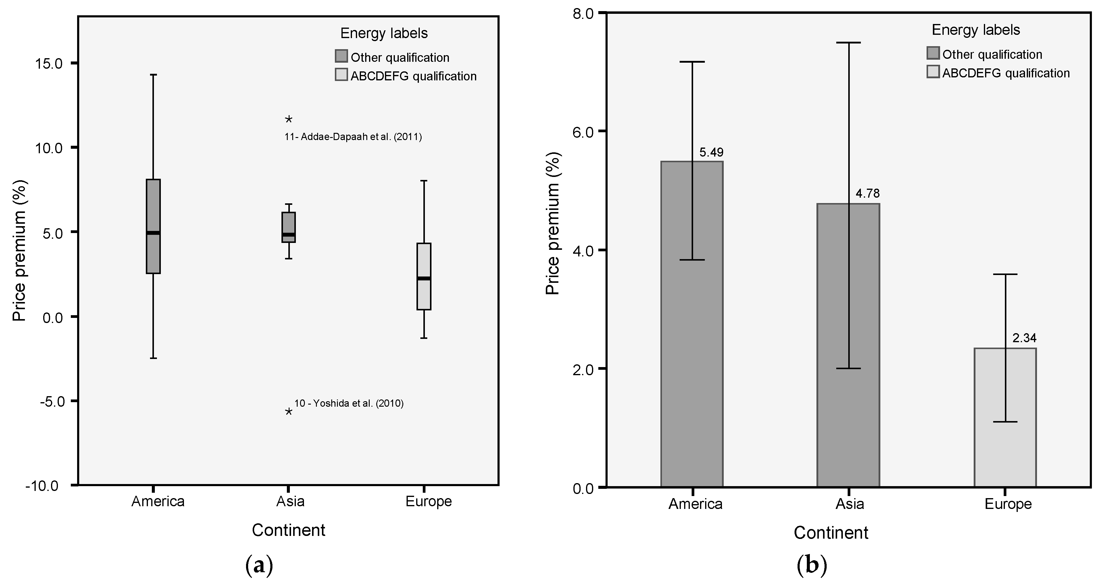
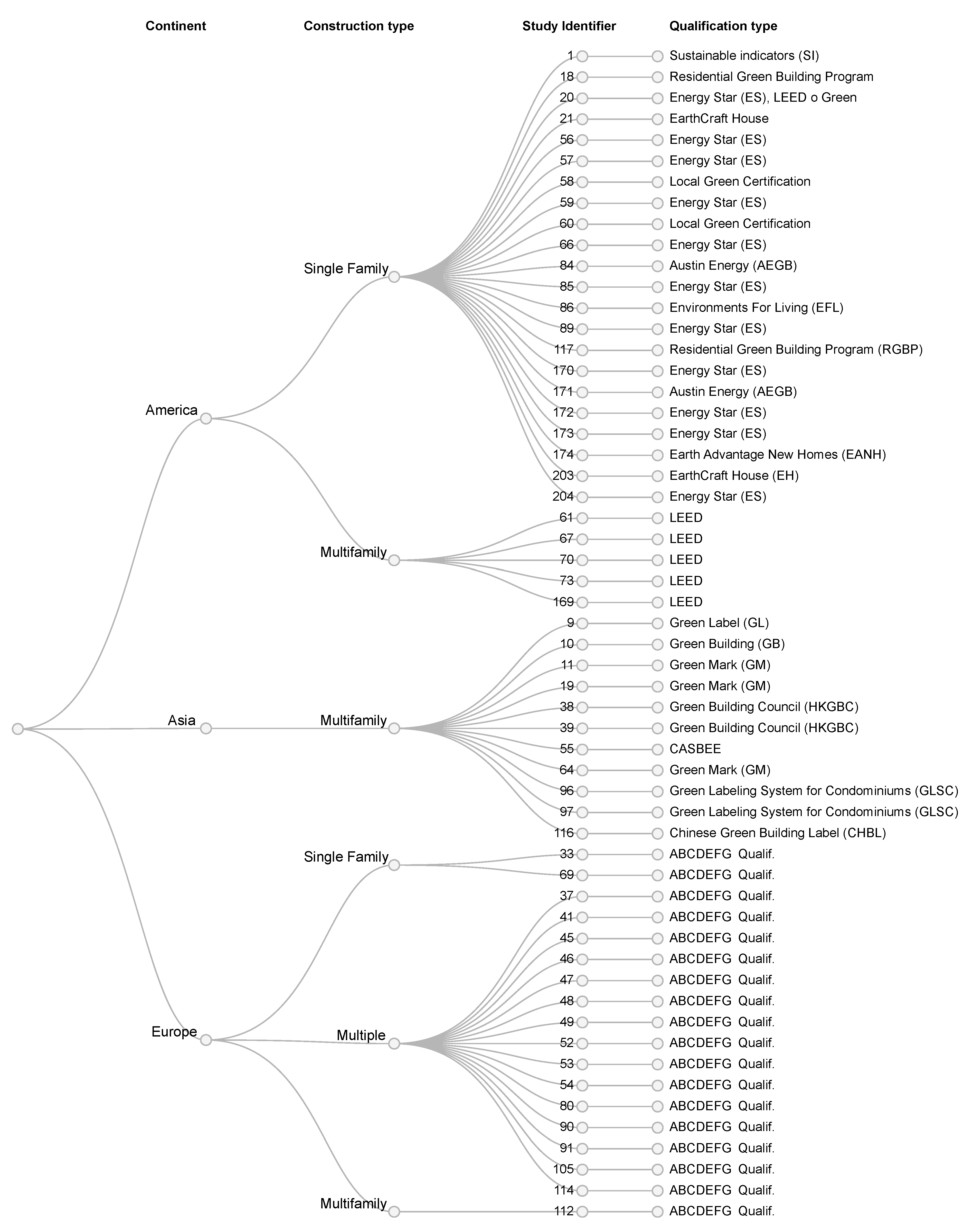
• The housing location and the type of EPC condition the value of the premium, with significant differences existing between the continents that were analyzed, mainly America and Asia, as compared to Europe. It has been estimated that the highest premiums are found in America at 5.36% and in Asia with 4.81%, while in Europe they are 2.32%;
• That of the data obtained in the analyzed documents, a meta-regression was conducted with various estimators, considering, as in the literature, that the REML is the most appropriate. It is observed that the variable having the greatest influence on the price premium is type of energy qualification (Qualif_ABCDEFG), with a decrease of 5.4% (B = −0.054) in the EPC with ABCDEFG qualifications as compared to other qualification types, as a result of the previous conclusion;
• That in housing with ABCDEFG qualifications, where the premium is analyzed upon changing from one value to another within the scale, the results are not conclusive, but they do suggest a trend, with the highest qualifications having higher premiums.

This document is useful in order to understand the current behavior on a global level. However, it has certain limitations due to combining data from distinct studies that are influenced by geographic area, type of qualification used, etc. Therefore, the results should be considered within the context of the analyzed documents and not as evidence of causality.

Furthering this line of knowledge is necessary and essential, so that discrimination between more and less efficient housing takes place in the market functioning (through prices). The price differential found in these studies suggests a major incentive to investment in energy efficiency, which, along with suitable policies, may contribute to eventually ensuring the commitments that these countries have made.

This review identified specific problems in the existing literature. Hopefully, these results will encourage researchers to use their own judgment as to the type of letter to be used as a reference, and to include all necessary data in order to replicate the study.

References

1. International Energy Agency. World Energy Outlook 2016; IEA Publications: Paris, France, 2016; p. 15. [Google Scholar]
2. IHOBE. Green Building Rating Systems: ¿Cómo Evaluar la Sostenibilidad en la Edificación? IHOBE Sociedad Pública de Gestión Ambiental: Bilbao, Spain, 2010; p. 72. [Google Scholar]
3. BREGlobal Limited. BREEAM International New Construction 2016; BREGlobal Limited: Watford/Hertfordshire, UK, 2016. [Google Scholar]
4. U.S. Green Building Council. LEED v4 for Homes Design and Construction; U.S. Green Building Council: Washington, DC, USA, 2013.
5. The European Parliament and the Council of the European Union. Directive 2002/91/EC of the European Parliament and of the Council of 16 December 2002 on the energy performance of buildings; European Union, Ed.; Official Journal of the European Communities: Aberdeen, UK, 2003; pp. 65–71. [Google Scholar]
6. The European Parliament and the Council of the European Union. Directive 2010/31/EU of the European Parliament and of the Council of 19 May 2010 on the Energy Performance of Buildings; European Union, Ed.; Official Journal of the European Union: Aberdeen, UK, 2010; pp. 13–35. [Google Scholar]
7. Passive House Institute. Passive House. Available online: https://passivehouse.com/index.html (accessed on 4 June 2019).
8. Yang, X. Measuring the Effects of Environmental Certification on Residential Property Values-Evidence from Green Condominiums in Portland. Ph.D. Thesis, Portland State University, Portland, OR, USA, 2013. [Google Scholar]
9. Yoshida, J.; Sugiura, A. The effects of multiple green factors on condominium prices. J. Real Estate Financ. Econ. 2015, 50, 412–437. [Google Scholar] [CrossRef]
10. Smith, M.L.; Glass, G.V. Meta-analysis of psychotherapy outcome studies. Am. Psychol. 1977, 32, 752–760. [Google Scholar] [CrossRef]
11. Hedges, L.V.; Olkin, I. Statistical Methods for Meta-Analysis; Press, A., Ed.; Academic Press: San Diego, CA, USA, 1985; p. 369. [Google Scholar] [CrossRef]
12. Lipsey, M.W.; Wilson, D.B. Practical Meta-Analysis; Sage Publications: Thousand Oaks, CA, USA, 2001. [Google Scholar]
13. Borenstein, M.; Hedges, L.V.; Higgins, J.P.T.; Rothstein, H.R. A basic introduction to fixed-effect and random-effects models for meta-analysis. Res. Synth. Methods 2010, 1, 97–111. [Google Scholar] [CrossRef]
14. Borenstein, M.; Higgins, J.P.T.; Hedges, L.V.; Rothstein, H.R. Basics of meta-analysis: I2 is not an absolute measure of heterogeneity. Res. Synth. Methods 2017, 8, 5–18. [Google Scholar] [CrossRef]
15. Rubio Aparicio, M.; Sánchez Meca, J.; Marín Martínez, F.; López López, J.A. Guidelines for reporting systematic reviews and meta-analyses. An. Psicol. 2018, 34, 412–420. [Google Scholar] [CrossRef]
16. Hunter, J.E.; Schmidt, F.L. Methods of Meta-Analysis: Correcting Error and Bias in Research Findings, 2nd ed.; Sage Publications: Thousand Oaks, CA, USA, 2004. [Google Scholar] [CrossRef]
17. Schmidt, F. What do data really mean? Research findings, meta-analysis, and cumulative knowledge in psychology. Am. Psychol. 1992, 47, 1173–1181. [Google Scholar] [CrossRef]
18. Eden, D. From the editors: Replication, meta-analysis, scientific progress, and AMJ’s publication policy. Acad. Manag. J. 2002, 45, 841–846. [Google Scholar] [CrossRef]
19. Ankamah-Yeboah, I.; Rehdanz, K. Explaining the Variation in the Value of Building Energy Efficiency Certificates: A Quantitative Metaanalysis; Kiel Working Papers 1949; Kiel Institute for the World Economy (IfW): Kiel, Germany, August 2014. [Google Scholar]
20. Brown, M.J.; Watkins, T. The “Green Premium” for Environmentally Certified Homes: A Meta-Analysis and Exploration. Researchgate Working Paper. 2016. Available online: https://www.researchgate.net/publication/294090858 (accessed on 11 July 2019).
21. Kim, S.; Lim, B.T.H.; Kim, J. Green features, symbolic values and rental premium: Systematic review and meta-analysis. Procedia Eng. 2017, 180, 41–48. [Google Scholar] [CrossRef]
22. Fizaine, F.; Voye, P.; Baumont, C. Does the literature support a high willingness to pay for green label buildings? An answer with treatment of publication bias. Rev. D’économie Polit. 2018, 128, 1013–1046. [Google Scholar] [CrossRef]
23. Liberati, A.; Altman, D.G.; Tetzlaff, J.; Mulrow, C.; Gøtzsche, P.C.; Ioannidis, J.P.A.; Clarke, M.; Devereaux, P.J.; Kleijnen, J.; Moher, D. The PRISMA statement for reporting systematic reviews and meta-analyses of studies that evaluate health care interventions: Explanation and elaboration. PLoS Med. 2009, 6, e1000100. [Google Scholar] [CrossRef]
24. Moher, D.; Liberati, A.; Tetzlaff, J.; Altman, D.G.; The, P.G. Preferred reporting items for systematic reviews and meta-analyses: The PRISMA statement. PLoS Med. 2009, 6, e1000097. [Google Scholar] [CrossRef] [PubMed]
25. Hyland, M.; Lyons, R.C.; Lyons, S. The value of domestic building energy efficiency - evidence from Ireland. Energy Econ. 2013, 40, 943–952. [Google Scholar] [CrossRef]
26. Mudgal, S.; Lyons, L.; Cohen, F.; Lyons, R.C.; Fedrigo-Fazio, D. Energy Performance Certificates in Buildings and their Impact on Transaction Prices and Rents in Selected EU Countries; Bio Intelligence Service: Paris, France, 2013; Volume 2013, p. 158. [Google Scholar]
27. Fuerst, F.; Warren-Myers, G. Does voluntary disclosure create a green lemon problem? Energy-efficiency ratings and house prices. Energy Econ. 2018, 74, 1–12. [Google Scholar] [CrossRef]
28. Soriano, F. Energy Efficiency Rating and House Price in the ACT; Commonwealth of Australia: Canberra, Australia, 2008; p. 56. ISBN 978-0-642-55422-2.
29. Olaussen, J.O.; Oust, A.; Solstad, J.T. Energy performance certificates—Informing the informed or the indifferent? Energy Policy 2017, 111, 246–254. [Google Scholar] [CrossRef]
30. Zheng, S.; Wu, J.; Kahn, M.E.; Deng, Y. The nascent market for “green” real estate in Beijing. Eur. Econ. Rev. 2012, 56, 974–984. [Google Scholar] [CrossRef]
31. Jensen, O.M.; Hansen, A.R.; Kragh, J. Market response to the public display of energy performance rating at property sales. Energy Policy 2016, 93, 229–235. [Google Scholar] [CrossRef]
32. Walls, M.; Gerarden, T.; Palmer, K.; Bak, X.F. Is energy efficiency capitalized into home prices? Evidence from three U.S. cities. J. Environ. Econ. Manag. 2017, 82, 104–124. [Google Scholar] [CrossRef]
33. Im, J.; Seo, Y.; Cetin, K.S.; Singh, J. Energy efficiency in U.S. residential rental housing: Adoption rates and impact on rent. Appl. Energy 2017, 205, 1021–1033. [Google Scholar] [CrossRef]
34. Salvi, M.; Horehájová, A.; Müri, R. Minergie Macht Sich Bezahlt; Universität Zürich: Zürich, Switzerland, 2008; p. 11. [Google Scholar]
35. Fuerst, F.; McAllister, P.; Nanda, A.; Wyatt, P. Energy performance ratings and house prices in Wales: An empirical study. Energy Policy 2016, 92, 20–33. [Google Scholar] [CrossRef]
36. Fuerst, F.; McAllister, P.; Nanda, A.; Wyatt, P. Does energy efficiency matter to home-buyers? An investigation of EPC ratings and transaction prices in England. Energy Econ. 2015, 48, 145–156. [Google Scholar] [CrossRef] [Green Version]
37. Shewmake, S.; Viscusi, W.K. Producer and consumer responses to green housing labels. Econ. Inq. 2015, 53, 681–699. [Google Scholar] [CrossRef]
38. Zhang, L.; Li, Y.; Stephenson, R.; Ashuri, B. Valuation of energy efficient certificates in buildings. Energy Build. 2018, 158, 1226–1240. [Google Scholar] [CrossRef]
39. de Ayala, A.; Galarraga, I.; Spadaro, J.V. The price of energy efficiency in the Spanish housing market. Energy Policy 2016, 94, 16–24. [Google Scholar] [CrossRef] [Green Version]
40. Shimizu, C. Will green Buildings Be Appropriately Valued by the Market? Reitaku University: Chiba, Japan, 2010; p. 30. [Google Scholar]
41. Yoshida, J.; Sugiura, A. Which “Greenness” is Valued? Evidence from Green Condominiums in Tokyo; Munich Personal RePEc Archive, MPRA: Munich, Germany, 2010; p. 33. [Google Scholar]
42. Aroul, R.R.; Hansz, J.A. The Value of “Green”: Evidence from the first mandatory residential green building program. J. Real Estate Res. 2012, 34, 27–50. [Google Scholar]
43. Högberg, L. The impact of energy performance on single-family home selling prices in Sweden. J. Eur. Real Estate Res. 2013, 6, 242–261. [Google Scholar] [CrossRef]
44. Davis, P.T.; McCord, J.; McCord, M.J.; Haran, M. Modelling the effect of energy performance certificate rating on property value in the Belfast housing market. Int. J. Hous. Mark. Anal. 2015, 8, 292–317. [Google Scholar] [CrossRef]
45. Notaries-France. La Valeur Verte des Logements en 2017; Étude Statistiques Immobilières, Métropolitaine: Paris, France, 2018; p. 11. [Google Scholar]
46. Neyeloff, J.L.; Fuchs, S.C.; Moreira, L.B. Meta-analyses and Forest plots using a microsoft excel spreadsheet: Step-by-step guide focusing on descriptive data analysis. BMC Res. Notes 2012, 5, 52. [Google Scholar] [CrossRef]
47. Martín Vallejo, J. Métodos Estadísticos en Meta-Análisis. Ph.D. Thesis, Universidad de Salamanca, Salamanca, Spain, 1995. [Google Scholar]
48. Faul, F. G*Power: Statistical Power Analyses for Windows and Mac; 3.1.9.2; Computer Programme: Kiel, Germany, 2014. [Google Scholar]
49. Amado, A.R. Capitalization of Energy Efficient Features Into Home Values in the Austin. Texas Real Estate Market. Ph.D. Thesis, Massachusetts Institute of Technology, Cambridge, MA, USA, 2007. [Google Scholar]
50. Salvi, M.; Horehájová, A.; Neeser, J. Der Minergie-Boom unter der Lupe; Universität Zürich: Zürich, Switzerland, 2010; p. 16. [Google Scholar]
51. Addae-Dapaah, K.; Chieh, S.J. Green mark certification: Does the market understand? J. Sustain. Real Estate 2011, 3, 162–191. [Google Scholar] [CrossRef]
52. Bloom, B.; Nobe, M.C.; Nobe, M.D. Valuing green home designs: A study of Energy Star® Homes. J. Sustain. Real Estate 2011, 3, 18. [Google Scholar]
53. Brounen, D.; Kok, N. On the economics of energy labels in the housing market. J. Environ. Econ. Manag. 2011, 62, 166–179. [Google Scholar] [CrossRef] [Green Version]
54. Deng, Y.; Li, Z.; Quigley, J.M. Economic returns to energy-efficient investments in the housing market: Evidence from Singapore. Reg. Sci. Urban Econ. 2012, 42, 506–515. [Google Scholar] [CrossRef] [Green Version]
55. Kahn, M.E.; Kok, N. The Value of Green Labels in the California Housing Market. Reg. Sci. Urban Econ. 2014, 47, 25–34. [Google Scholar] [CrossRef]
56. Stephenson, R.M. Quantifying the Effect of Green Building Certification on Housing Prices in Metropolitan Atlanta. Ph.D. Thesis, Georgia Institute of Technology, Atlanta, GA, USA, 2012. [Google Scholar]
57. Cajias, M.; Piazolo, D. Green performs better: Energy efficiency and financial return on buildings. J. Corp. Real Estate 2013, 15, 53–72. [Google Scholar] [CrossRef]
58. Feige, A.; McAllister, P.; Wallbaum, H. Rental price and sustainability ratings: Which sustainability criteria are really paying back? Constr. Manag. Econ. 2013, 31, 322–334. [Google Scholar] [CrossRef]
59. Fuerst, F.; McAllister, P.; Nanda, A.; Wyatt, P. An Investigation of the Effect of EPC Ratings on House Prices; 13D/148; Department of Energy & Climate Change: London, UK, 2013; p. 41.
60. Jayantha, W.M.; Wan Sze, M. Effect of green labelling on residential property price: A case study in Hong Kong. J. Facil. Manag. 2013, 11, 31–51. [Google Scholar] [CrossRef]
61. Shimizu, C. Sustainable measures and economic value in green housing. Open House Int. 2013, 38, 57–63. [Google Scholar]
62. Walls, M.; Palmer, K.; Gerarden, T. Is Energy Efficiency Capitalized into Home Prices? Evidence from Three US Cities. SSRN Electron. J. 2013. [Google Scholar] [CrossRef] [Green Version]
63. Cerin, P.; Hassel, L.G.; Semenova, N. Energy performance and housing prices. Sustain. Dev. 2014, 22, 404–419. [Google Scholar] [CrossRef]
64. Deng, Y.; Wu, J. Economic returns to residential green building investment: The developers’ perspective. Reg. Sci. Urban Econ. 2014, 47, 35–44. [Google Scholar] [CrossRef]
65. Fuerst, F.; Shimizu, C. The rise of eco-labels in the Japanese housing market. J. Jpn. Int. Econ. 2016, 39, 108–122. [Google Scholar] [CrossRef]
66. Kahn, M.E.; Kok, N. The capitalization of green labels in the California housing market. Reg. Sci. Urban Econ. 2014, 47, 25–34. [Google Scholar] [CrossRef]
67. Rahman, F. Do Green Buildings Capture Higher Market-Values and Prices? A Case-Study of LEED and BOMA-BEST Properties. Ph.D. Thesis, University of Waterloo, Waterloo, ON, Canada, 2014. [Google Scholar]
68. Bonifaci, P.; Copiello, S. Price premium for buildings energy efficiency: Empirical findings from a hedonic model. Valori E Valutazioni 2015, 14, 5–15. [Google Scholar]
69. DePratto, B. The Market Benefits of Green Condos in Toronto for Educational Purposes, Special Report TD Economics. 2015. Available online: https://www.td.com/document/PDF/economics/special/GreenCondos.pdf (accessed on 15 June 2019).
70. Fregonara, E.; Rolando, D.; Semeraro, P.; Vella, M. The impact of Energy Performance Certificate level on house listing prices. First evidence from Italian real estate. Aestimum 2015, 65, 143–163. [Google Scholar] [CrossRef]
71. Freybote, J.; Sun, H.; Yang, X. The Impact of LEED Neighborhood Certification on Condo Prices. Real Estate Econ. 2015, 43, 586–608. [Google Scholar] [CrossRef]
72. Ramos, A.; Pérez Alonso, A.; Silva, S. Valuing energy performance certificates in the Portuguese residential. Work. Pap. Rscas 2015, 2015, 36. [Google Scholar]
73. Bond, S.A.; Devine, A. Certification matters: Is green talk cheap talk? J. Real Estate Financ. Econ. 2016, 52, 117–140. [Google Scholar] [CrossRef]
74. Bruegge, C.; Carrión Flores, C.E.; Pope, J.C. Does the housing market value energy efficient homes? Evidence from the energy star program. Reg. Sci. Urban Econ. 2016, 57, 63–76. [Google Scholar] [CrossRef]
75. Chegut, A.; Eichholtz, P.; Holtermans, R. Energy efficiency and economic value in affordable housing. Energy Policy 2016, 97, 39–49. [Google Scholar] [CrossRef]
76. Fuerst, F.; Shimizu, C. Green luxury goods? The economics of eco-labels in the Japanese housing market. J. Jpn. Int. Econ. 2016, 39, 108–122. [Google Scholar] [CrossRef]
77. Kempf, C. How Green Buildings Mitigate Risk. Ph.D. Thesis, University of Zurich, Zurich, Switzerland, 2016. [Google Scholar]
78. Marmolejo Duarte, C. La incidencia de la calificación energética sobre los valores residenciales: Un análisis para el mercado plurifamiliar en Barcelona. Inf. Construcción 2016, 68, e156. [Google Scholar] [CrossRef]
79. Stanley, S.; Lyons, R.C.; Lyons, S. The price effect of building energy ratings in the Dublin residential market. Energy Effic. 2016, 9, 875–885. [Google Scholar] [CrossRef]
80. Zhang, L.; Liu, H.; Wu, J. The price premium for green-labelled housing: Evidence from China. Urban Stud. 2016, 54, 3524–3541. [Google Scholar] [CrossRef]
81. Aroul, R.R.; Rodríguez, M. The increasing value of green for residential real estate. J. Sustain. Real Estate 2017, 9, 19. [Google Scholar]
82. Dressler, L.; Cornago, E. The Rent Impact of Disclosing Energy Performance Certificates: Energy Efficiency and Information Effects; ECARES Working Paper; Université Libre de Bruxelles: Bruxelles, Belgium, 2017; p. 44. [Google Scholar]
83. Hui, E.C.-m.; Tse, C.-k.; Ka-hung, Y. The effect of beam plus certification on property price in Hong Kong. Int. J. Strateg. Prop. Manag. 2017, 21, 384–400. [Google Scholar] [CrossRef]
84. Kholodilin, K.A.; Mense, A.; Michelsen, C. The market value of energy efficiency in buildings and the mode of tenure. Urban Stud. 2017, 54, 3218–3238. [Google Scholar] [CrossRef]
85. Notaries-France. La Valeur Verte des Logements en 2016; Étude Statistiques Immobilières, Métropolitaine: Paris, France, 2017; p. 4. [Google Scholar]
86. Pride, D.J.; Little, J.M.; Mueller-Stoffels, M. The value of energy efficiency in the anchorage residential property market. J. Sustain. Real Estate 2017, 9, 23. [Google Scholar]
87. Rahman, F.; Rowlands, I.; Weber, O. Do green buildings capture higher market valuations and lower vacancy rates? A Canadian case study of LEED and BOMA-BEST properties. Smart Sustain. Built Environ. 2017, 6, 102–115. [Google Scholar] [CrossRef]
88. Cornago, E.; Dressler, L. Incentives to (not) Disclose Energy Performance Information in the Housing Market; ECARES Working Paper; Université libre de Bruxelles: Bruxelles, Belgium, 2018; p. 50. [Google Scholar]
89. Cajias, M.; Fuerst, F.; Bienert, S. Tearing down the information barrier: The price impacts of energy efficiency ratings for buildings in the German rental market. Energy Res. Soc. Sci. 2019, 47, 177–191. [Google Scholar] [CrossRef]
90. Taltavull de La Paz, P.; Perez-Sanchez, R.V.; Mora-Garcia, R.-T.; Perez-Sanchez, J.-C. Green premium evidence from climatic areas: A case in Southern Europe, Alicante (Spain). Sustainability 2019, 11, 686. [Google Scholar] [CrossRef]
91. Marmolejo Duarte, C.; Chen, A. La incidencia de las etiquetas energéticas EPC en el mercado plurifamiliar español: Un análisis para Barcelona, Valencia y Alicante. Ciudad Territ. Estud. Territ. 2019, 51, 101–118. [Google Scholar]
92. Hair, J.F.; Anderson, R.E.; Tatham, R.L.; Black, W.C. Análisis Multivariante, 5th ed.; Prentice Hall: Madrid, Spain, 2008. [Google Scholar]
93. Doucouliagos, H.; Stanley, T.D. Publication selection bias in minimum-wage research? a meta-regression analysis. Br. J. Ind. Relat. 2009, 47, 406–428. [Google Scholar] [CrossRef]
94. Begg, C.B. Publication bias. In The Handbook of Research Synthesis; Russell Sage Foundation: New York, NY, USA, 1994; pp. 399–409. [Google Scholar]
95. Greene, W.H. Econometric Analysis, 5th ed.; Prentice Hall: Upper Saddle River, NJ, USA, 2003. [Google Scholar]
96. Sousa, M.R.d.; Ribeiro, A.L.P. Revisão sistemática e meta-análise de estudos de diagnóstico e prognóstico: Um tutorial. Arq. Bras. Cardiol. 2009, 92, 241–251. [Google Scholar] [CrossRef] [PubMed]
97. Núñez Serrano, J.A. El Efecto de la Accesibilidad a Los Mercados en la Eficiencia Empresarial. Una Aproximación Microeconómica. Ph.D. Thesis, Complutense de Madrid, Madrid, Spain, 2013. [Google Scholar]
98. Adame García, V.; Alonso Meseguer, J.; Pérez Ortiz, L.; Tuesta, D. Infraestructuras y Crecimiento: Un Ejercicio de Meta-Análisis; BBVA Research: Madrid, Spain, 2017; p. 30. [Google Scholar]
99. Pértega Díaz, S.; Pita Fernández, S. Revisiones sistemáticas y Metaanálisis (II). Cad. Aten. Primaria 2005, 12, 166–171. [Google Scholar]
100. López Cuadrado, M.T. Meta-Análisis: Aportación Metodológica en la Investigación de Resultados de Salud. Ph.D. Thesis, Universidad Autonoma de Madrid, Madrid, Spain, 2011. [Google Scholar]
101. DerSimonian, R.; Laird, N. Meta-analysis in clinical trials. Control. Clin. Trials 1986, 7, 177–188. [Google Scholar] [CrossRef]
102. Viechtbauer, W. Bias and efficiency of meta-analytic variance estimators in the random-effects model. J. Educ. Behav. Stat. 2005, 30, 261–293. [Google Scholar] [CrossRef]
103. Veroniki, A.A.; Jackson, D.; Viechtbauer, W.; Bender, R.; Bowden, J.; Knapp, G.; Kuss, O.; Higgins, J.P.; Langan, D.; Salanti, G. Methods to estimate the between-study variance and its uncertainty in meta-analysis. Res. Synth. Methods 2016, 7, 55–79. [Google Scholar] [CrossRef]
104. Wallace, B.C.; Lajeunesse, M.J.; Dietz, G.; Dahabreh, I.J.; Trikalinos, T.A.; Schmid, C.H.; Gurevitch, J. OpenMEE: Intuitive, open-source software for meta-analysis in ecology and evolutionary biology. Methods Ecol. Evol. 2017, 8, 941–947. [Google Scholar] [CrossRef]
105. Viechtbauer, W. Conducting Meta-Analyses in R with the metafor Package. J. Stat. Softw. 2010, 36, 48. [Google Scholar] [CrossRef]
106. Daryanto, A. Test de Breusch-Pagan y Koenker 2. Computer programme. 2018. Available online: https://www.statisticshowto.datasciencecentral.com/breusch-pagan-godfrey-test/ (accessed on 25 May 2019).
107. Peters, J.L.; Sutton, A.J.; Jones, D.R.; Abrams, K.R.; Rushton, L. Contour-enhanced meta-analysis funnel plots help distinguish publication bias from other causes of asymmetry. J. Clin. Epidemiol. 2008, 61, 991–996. [Google Scholar] [CrossRef]
108. Baujat, B.; Mahé, C.; Pignon, J.-P.; Hill, C. A graphical method for exploring heterogeneity in meta-analyses: Application to a meta-analysis of 65 trials. Stat. Med. 2002, 21, 2641–2652. [Google Scholar] [CrossRef]
109. Servicio Gallego de Salud. Meta-Análisis; Servicio Gallego de Salud: Galicia, Spain, 2015; p. 31.
110. Iberoamericano, C.C. Manual Cochrane de Revisiones Sistemáticas de Intervenciones; Centro Cochrane Iberoamericano: Barcelona, Spain, 2011; Volume 5.1.0. [Google Scholar]
111. Camilli Trujillo, C. Aprendizaje Cooperativo e Individual en el Rendimiento Académico en Estudiantes Universitarios: Un Meta-Análisis. Ph.D. Thesis, Universidad Complutense de Madrid, Madrid, Spain, 2015. [Google Scholar]
112. Higgins, J.P.T.; Thompson, S.G.; Deeks, J.J.; Altman, D.G. Measuring inconsistency in meta-analyses. BMJ Clin. Res. Ed. 2003, 327, 557–560. [Google Scholar] [CrossRef] [PubMed] [Green Version]
113. Mauri, M.; Elli, T.; Caviglia, G.; Uboldi, G.; Azzi, M. RAWGraphs: A visualisation platform to create open outputs. In Proceedings of the 12th Biannual Conference on Italian SIGCHI Chapter, Cagliari, Italy, 18–20 September 2017; pp. 1–5. [Google Scholar]
114. Thompson, S.G.; Sharp, S.J. Explaining heterogeneity in meta-analysis: A comparison of methods. Stat. Med. 1999, 18, 2693–2708. [Google Scholar] [CrossRef]
115. Nelson, J.P.; Kennedy, P.E. The Use (and Abuse) of Meta-analysis in environmental and natural resource economics: An assessment. Environ. Resour. Econ. 2009, 42, 345–377. [Google Scholar] [CrossRef]
Figure 1. Geographic distribution of the assessment systems on a global level. Source: IHOBE [2].
Sustainability 11 06303 g001
Figure 2. Geographic distribution of the assessment systems on a European level. The ABCDEFG qualification is applicable in the member countries of the EU. Source: IHOBE [2].
Sustainability 11 06303 g002
Figure 3. Structuring process of the registers in the created database.
Sustainability 11 06303 g003
Figure 4. PRISMA Flow Diagram. Selection process for the documents, classification of the registers and definition of the analyses made.
Sustainability 11 06303 g004
Figure 5. Geographic distribution of the documents analyzed based on continents.
Sustainability 11 06303 g005
Figure 6. (a) Box and whisker plot of the premium in the sales price (%); and (b) bar graph with the mean and the CI (95%) of the sales price premium (%) based on the type of energy label and continent.
Sustainability 11 06303 g006
Figure 7. (a) Histogram and normal curve of the dependent variable (Premium_EPC); (b) P-P plot of residual normality.
Sustainability 11 06303 g007
Figure 8. (a) Funnel plot for the random effects model; and (b) Baujat plot for the final sample of 56 registers.
Sustainability 11 06303 g008
Figure 9. Forest plot of the analysis of influence of the studies.
Sustainability 11 06303 g009
Figure 10. Forest plot based on publication type and overall combined effect.
Sustainability 11 06303 g010
Figure 11. Forest plot based on period of data collection and overall combined effect.
Sustainability 11 06303 g011
Figure 12. Forest plot by continent and overall combined effect.
Sustainability 11 06303 g012
Figure 13. Distribution of data continent, construction type, number of registers (study identifier according to Table 1), and type of energy label. Representation made with the RAWGraphs web tool [113].
Sustainability 11 06303 g013
Figure 14. Bar graph of the premiums as a percentage of the sales price for buildings with the ABCDEFG qualification, based on the analyzed letter grouping.
Sustainability 11 06303 g014
Figure 15. Bar graphs with the sale price premiums of the properties (%) and CI (95%), with the ABCDEFG qualification, based on the reference value: (a) Letter D, (b) letter F, (c) letter G, and (d) letter NT (no label). NOTE: The values between parentheses are the number of cases for this letter. E.g.: A (n = 5): 15.70%; G (Ref.). Qualification letter A with 5 cases to obtain a mean premium of 15.70% when the reference letter is G.
Sustainability 11 06303 g015aSustainability 11 06303 g015b