Minimizing the Risks of Highway Transport of Hazardous Materials

Abstract

Many key industrial and scientific processes, such as the generation of nuclear energy, are of enormous social benefit as energy demand and consumption grow over time. However, a drawback of several such processes is the production of hazardous waste materials, which often requires transportation along highway networks to treatment or disposal facilities. This waste can represent a safety hazard to civilians located along the transportation route. Most prior literature in this domain considers risk within only a single facet, and thus several important risk factors may not be considered. In our paper, we propose a multi-objective program to allow for the analysis and selection of minimally risky routes for hazardous materials transportation. The model assesses risk factors including the length of the selected route, the total population in areas surrounding the selected route, and the likelihood of an accident occurring along the selected route. Our paper uniquely uses geographic information systems (GIS) technology to model this optimization problem. This approach allows us to model risk along multiple dimensions simultaneously. We collect empirical data to test the model and present a case study for risk mitigation using a study area located in California. We show that our multi-objective approach is effective in presenting the decision-maker with a portfolio of solutions that perform well via each factor.

1. Introduction

Industrial and scientific processes offer enormous promise to contemporary society but often result in unusable and potentially dangerous byproducts. These substances, often dubbed hazardous materials, present enormous logistical challenges for organizations that need to dispose of them without subjecting human populations and the environment to undue risk [1,2,3]. Waste is often categorized as hazardous if it meets any of four common criteria: ignitability, corrosiveness, reactivity, or toxicity [4]. Unfortunately, the generation of hazardous waste is an inherent problem in many industrial processes, ranging from waste created by nuclear power plants [5] to the byproducts of manufacturing lines [6].

The safe disposal of these materials is crucial for ensuring that humans do not encounter potentially dangerous and life-threatening chemicals. While highway infrastructure may ultimately allow for the fastest viable transportation of these materials to their eventual disposal sites, it also poses significant risks to human safety in the event of a traffic accident or unintended leakage [7]. In many cases, local, state, and federal laws dictate that highway routing schemes for transportation of hazardous materials must be designed to preserve human safety. These laws generally serve two purposes: first, to ban transportation of hazardous materials along specific road segments, and second, to establish legal liability of the transporter in the event of an accident. In the United States, the Hazardous Materials Transportation Act (HMTA), enacted in 1975, is the most widely known such law on a federal level [8]. Additional restrictions are required by state laws, but it is often unclear how to reach optimal routing decisions as each routing problem is unique and multi-faceted [9].

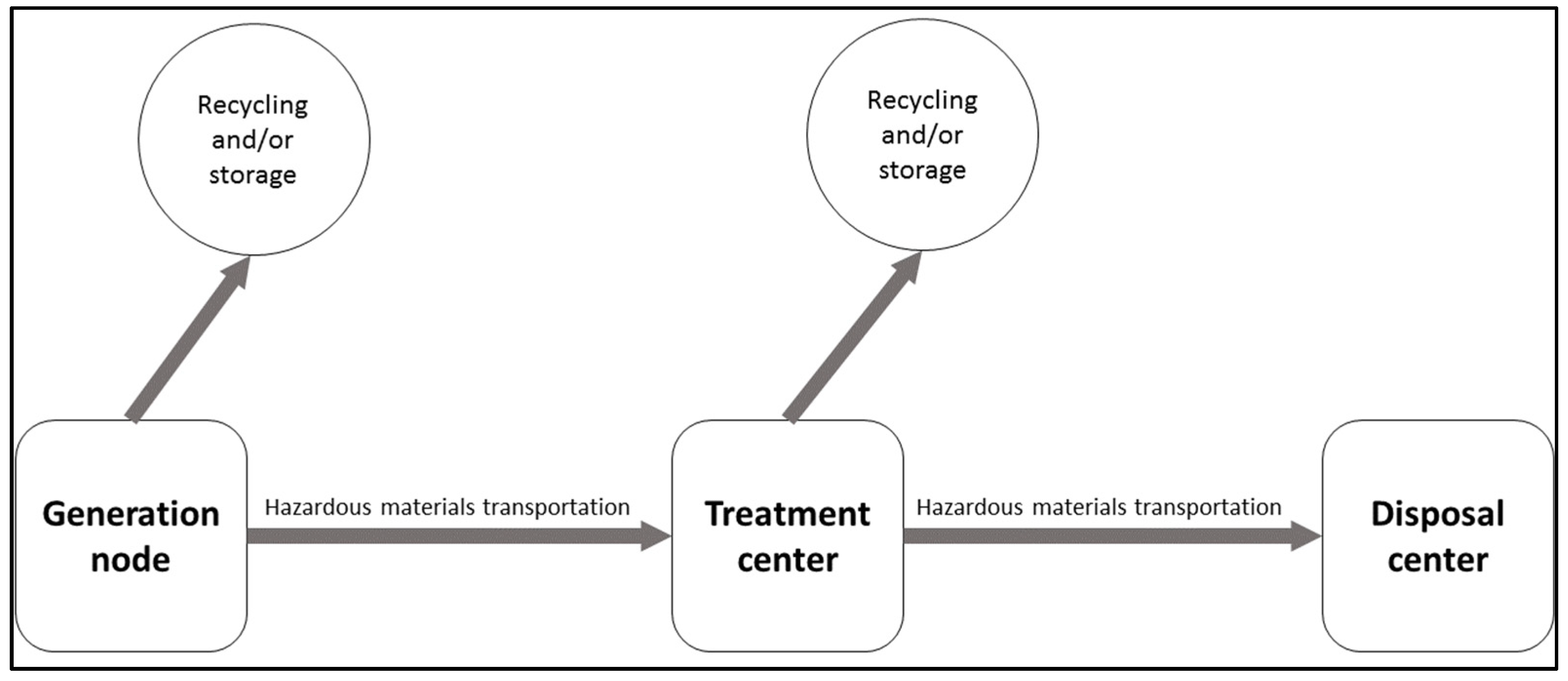
The parameters of this problem suggest that some hazardous waste must be transported from an origin facility to some destination. For most types of hazardous waste, individual parcels or barrels of waste are processed at three unique facilities [10]. The “generation node,” such as an industrial facility, first creates hazardous waste. At this facility, some of the waste may be recycled or kept in storage. The remainder of the waste is then transported to a treatment center, within which the waste is chemically altered to mitigate some of its dangerous properties. Within this site, some of the waste may, again, be recycled or kept in storage. Finally, the remainder of the waste is transported to a disposal center, where it is safely processed. Figure 1 displays a schematic of this hazardous materials management program.

As a result of this hazardous materials management scheme, many hazardous materials are actually transported twice after they are created. The first time these materials are transported, they are particularly dangerous, as they likely have not been processed in any way so as to make them less harmful in the event of human exposure. The second time that these materials are transported, they have been treated, so they often represent slightly less dangerous versions of the initial compounds, although they may still threaten human safety.

2. Literature Review

The objective of a hazardous materials management program is “to ensure safe, efficient and cost-effective collection, transportation, treatment and disposal of wastes” [11]. Indeed, many local, state, and national laws, such as HMTA, require that these materials be transported so as to avoid risks to human safety [8]. The literature has discussed the concern over hazardous materials’ transportation in previous years. The most similar work to ours [12] proposes considering both traffic considerations and the extent of the exposed population. Past work has modeled the spread of hazardous waste from a potential accident zone such as a Gaussian Plume [13]. Studies have also focused on the routing problem from a profit-oriented perspective. For example, prior work has attempted to minimize the various potential sources of costs to the transportation company [14].

Although the literature has established the potential severity of accidents involving hazardous materials and has suggested some ways in which companies may transport these materials economically, it has not established a method by which safe modes of transportation for these materials ought to be selected. We acknowledge that profit-oriented perspectives are valuable, but we also note that the enormous prevalence of accidents involving hazardous materials indicates the need for safer routes for hazardous materials transportation. Since 2000, the Department of Transportation’s Office of Hazardous Materials Safety (OHMS) has recorded nearly 300,000 incidents of hazardous materials accidents along highway routes in the United States [15]. We argue that selecting for safer hazardous materials routes implies that companies may improve profit by preventing costly delays or eventual lawsuits that may result from accidents in hazardous materials transportation; at the same time, companies may preserve their goodwill by altruistically aiming to preserve human safety.

Previous research provides us with an excellent basis on which to build [4,11,13,14,16,17,18]. At present, much of the literature has focused on either the direct costs of hazardous materials transportation or quantifying possible losses in the event of an accident. The state-of-the-art approaches to routing often treat risk as a single measure, if risk is considered at all [19]. However, in practice, risk is multi-faceted, and decision-makers are often faced with tradeoffs between several risk factors. Thus, in this work, we believe that we can make a significant contribution by building an advanced mathematical model involving multi-objective programming (MOP), which minimizes the risk of transportation along highway networks. Using our model, the decision-maker can specify which risk factors are most important to mitigate and a customized weighting scheme among the three objectives.

3. Materials and Methods

The formulation of our mathematical program is grounded in linear transportation or “resource flow” models. Although we propose solving a series of models to allow for a multi-objective program (MOP), each model will represent a version of the common “shortest-path” transportation model. In each linear program, however, we will focus our model on a different objective function. In this type of linear program, we interpret a highway network as an interconnected set of “nodes” or intersections between various “arcs” or road segments.

Let $N$ represent the set of all possible nodes within a selected study area. For each possible node $k$ within the study area, we introduce one flow conservation constraint in the model representing the net flow at that node, or the sum of the inflow minus the sum of the outflow. We represent whether an arc is active with a variable $Y_{ij}$, which equals 1 if the arc from i to j is active and 0 otherwise. At the vast majority of nodes, the sum of the inflow should exactly equal the sum of the outflow (inflow minus outflow equals zero). Two exceptions occur at the initial supply or origin node, $s$, and the final demand or destination node, $t$, at which we use right-hand sides of ‒1 and 1 to ensure that the model must choose a path through the network. Additionally, a further property of this shortest-path transportation model is that this constraint ensures binary or integer constraints are unnecessary, as variables are all assigned a 0 or 1 value inherently as a result of the transportation formulation [20]. This facet of the model reduces its computational complexity and, therefore, its computation time. We formulate Equation (1) below, representing the flow conservation constraint:

$${{\displaystyle \sum }}_{i:\left(i,k\right)\in N}\left(Y_{ik}\right)-{{\displaystyle \sum }}_{j:\left(j,k\right)\in N}\left(Y_{kj}\right)=\{\begin{array}{c}-1\hspace{1em}i=t,t\\ -0\hspace{1em}i\ne s,t\\ -1\hspace{1em}i=s,s\end{array}.$$

(1)

Next, we consider each of three possible objectives that a decision-maker may consider as they attempt to minimize risk in the transportation of hazardous materials along highway networks. The first such source of risk concerns the distance that a vehicle carrying hazardous materials must travel from its start node to its terminating node. The minimization of this function is important for several reasons. First, in order to minimize costs, the decision-maker may look to avoid gas or labor costs associated with longer routes. Second, it is also possible that longer routes impose additional risk, as they invite further possibilities for traffic accidents or other spills of hazardous materials. Recognizing these concerns, we formulate in Equation (2) the first of the three objectives, which computes $D$, the sum of distances, $d_{ij}$, traversed along active arcs:

$$D={{\displaystyle \sum }}_{\left(i,j\right)\in N}{Y}_{ij}{d}_{ij}.$$

(2)

The next objective concerns the possibility of exposing the civilian population to harmful hazardous materials in the event of a traffic accident. Should an accident occur, the decision-maker should stipulate that as few individuals as possible be exposed to the hazardous materials. This objective serves an altruistic purpose but may also limit the legal liability of the decision-maker or their organization in the event of an accident. Recognizing these concerns, we formulate in Equation (3) the second objective, which computes $P$, the sum of populations, $p_{ij}$, potentially exposed along active arcs:

$$P={{\displaystyle \sum }}_{\left(i,j\right)\in N}{Y}_{ij}{p}_{ij}.$$

(3)

Third, we consider an objective measuring the risk that an accident will occur along the selected route for the transportation of hazardous materials. Due to the design of various roadways, traffic patterns, and other factors, accidents are more likely when traveling along some roads than others [21]. For example, when comparing two roads of similar lengths, one may find that visibility is superior on one road compared to the other, thereby minimizing the chance that an accident will occur. The decision-maker may wish to minimize the risk of an accident so as to promote public safety and ensure that the hazardous materials reach their destination successfully.

The first and simplest strategy to define this function is to use the raw number of hazardous materials accidents along each road as representative of “accident risk” so that a road on which two accidents have occurred is twice as risky as a road on which a single accident has occurred. We can model this objective in the same structure as the previous two objectives, which is advantageous. However, the disadvantage of this strategy is that it essentially assumes that each route is equally utilized. A road on which two accidents have occurred may be twice as risky as a route on which one accident has occurred if both routes have been used for the same number of journeys, but not if the first route happens to be utilized twice as much.

As such, a second strategy is to calculate the proportion of drives along a particular route that result in accidents. Assuming that these proportions represent independent probabilities, we can calculate our objective function (the probability of at least one accident occurring) as one minus the probability of no accidents occurring. After assigning each arc the empirically calculated probability of an accident occurring, $a_{ij}$, we compute in Equation (4) the probability of at least one accident occurring between the initial node and the final node:

$$A=1-\left[{{\displaystyle \prod }}_{\left(i,j\right)\in N}(1-Y_{ij}{a}_{ij})\right].$$

(4)

However, note that Equation (4) represents a non-linear function, which requires the use of more advanced solution techniques and almost certainly increases solve times. While various algorithms exist to solve non-linear models, these methods are generally more complex than their linear counterparts. To assuage this concern, we propose in Equation (5) a linearized function that equivalently minimizes the same probability:

$$A={{\displaystyle \sum }}_{\left(i,j\right)\in N}-Y_{ij}LOG\left(1-a_{ij}\right).$$

(5)

To represent each of these objectives in a multi-objective formulation within the same model, we must solve several models in sequence. First, subject to Equation (1), we minimize each of Equations (2), (3), and (5) in the first stage of our process. In each solution, only one objective is considered, and the other two are disregarded. We record the optimal values of each objective for reference in the further stages of the optimization process.

Next, we define ${\phi }_D$, ${\phi }_P$, and ${\phi }_A$ in Equations (6), (7), and (8) as the percentage difference between a solution and the optimum reached when minimizing an objective in isolation (denoted *):

$${\phi }_D=\frac{\left({{\displaystyle \sum }}_{\left(i,j\right)\in N}{Y}_{ij}{d}_{ij}\right)-{\left({{\displaystyle \sum }}_{\left(i,j\right)\in N}{Y}_{ij}{d}_{ij}\right)}^{*D}}{{\left({{\displaystyle \sum }}_{\left(i,j\right)\in N}{Y}_{ij}{d}_{ij}\right)}^{*D}}$$

(6)

$${\phi }_P=\frac{\left({{\displaystyle \sum }}_{\left(i,j\right)\in N}{Y}_{ij}{p}_{ij}\right)-{\left({{\displaystyle \sum }}_{\left(i,j\right)\in N}{Y}_{ij}{p}_{ij}\right)}^{*P}}{{\left({{\displaystyle \sum }}_{\left(i,j\right)\in N}{Y}_{ij}{p}_{ij}\right)}^{*P}}$$

(7)

$${\phi }_A=\frac{\left({{\displaystyle \sum }}_{\left(i,j\right)\in N}-Y_{ij}LOG\left(1-a_{ij}\right)\right)-{\left({{\displaystyle \sum }}_{\left(i,j\right)\in N}-Y_{ij}LOG\left(1-a_{ij}\right)\right)}^{*A}}{{\left({{\displaystyle \sum }}_{\left(i,j\right)\in N}-Y_{ij}LOG\left(1-a_{ij}\right)\right)}^{*A}}.$$

(8)

Next, the decision-maker specifies three weights for the different objectives in Equation (9), which sum to 1. Weights $w_D$, $w_P$, and $w_A$ signify the relative importance of distance, population, and accident risks, respectively. These variables are typically prespecified by the user and serve as constants in the instantiated model rather than true decision-making variables. Setting a weight to 1 optimizes a singular objective and produces the same optimal routing decision as solving that specific model in the previous phase.

$$w_D+w_P+w_A=1$$

(9)

The weights are specified by the decision-maker and may vary depending upon the application. For example, if the decision-maker is considering the transportation of particularly hazardous materials and is concerned about the prospect of exposure, they may wish to put more emphasis on the accident and population objectives. For instance, they may choose a weight of 0.40 for accidents, 0.40 for population, and 0.20 for distance. On the other hand, a different use case may be if a decision-maker has less hazardous materials but is more concerned with economic considerations. For instance, they may choose weights of 0.10 for accidents, 0.10 for population, and 0.80 for distance. These specific choices reflect the relative emphasis that the decision-maker wishes to place upon each factor. For the purposes of our paper, we do not assume a particular emphasis; instead, we weight each factor equally at one-third.

Finally, we define $Z$ to evaluate solutions via the sum of the weighted deviations from the respective optimal. $Z$ is minimized to solve the multi-objective formulation:

$$Z={\phi }_D{w}_D+{\phi }_P{w}_P+{\phi }_A{w}_A.$$

(10)

Table 1. Summary of model sequence in multi-objective formulation.

Step	Objective	Model Formulation
1	Distance	Minimize $D={{\displaystyle \sum }}_{\left(i,j\right)\in N}{Y}_{ij}{d}_{ij}$ subject to: ${\displaystyle {\displaystyle \sum }_{i:\left(i,k\right)\in N}}\left(Y_{ik}\right)-{\displaystyle {\displaystyle \sum }_{j:\left(j,k\right)\in N}}\left(Y_{kj}\right)=\{\begin{array}{c}-1\hspace{1em}i=t,t\\ -0\hspace{1em}i\ne s,t\\ -1\hspace{1em}i=s,s\end{array}$ And $Y_{ij}\ge 0\forall i,j$
1	Population	Minimize $P={{\displaystyle \sum }}_{\left(i,j\right)\in N}{Y}_{ij}{p}_{ij}$ subject to: ${\displaystyle {\displaystyle \sum }_{i:\left(i,k\right)\in N}}\left(Y_{ik}\right)-{\displaystyle {\displaystyle \sum }_{j:\left(j,k\right)\in N}}\left(Y_{kj}\right)=\{\begin{array}{c}-1\hspace{1em}i=t,t\\ -0\hspace{1em}i\ne s,t\\ -1\hspace{1em}i=s,s\end{array}$ And $Y_{ij}\ge 0\forall i,j$
1	Accidents	Minimize $A={{\displaystyle \sum }}_{\left(i,j\right)\in N}-Y_{ij}LOG\left(1-a_{ij}\right)$ subject to: ${\displaystyle {\displaystyle \sum }_{i:\left(i,k\right)\in N}}\left(Y_{ik}\right)-{\displaystyle {\displaystyle \sum }_{j:\left(j,k\right)\in N}}\left(Y_{kj}\right)=\{\begin{array}{c}-1\hspace{1em}i=t,t\\ -0\hspace{1em}i\ne s,t\\ -1\hspace{1em}i=s,s\end{array}$ And $Y_{ij}\ge 0\forall i,j$
2	Multi-objective	Minimize $Z={\phi }_D{w}_D+{\phi }_P{w}_P+{\phi }_A{w}_A$ subject to: ${\displaystyle {\displaystyle \sum }_{i:\left(i,k\right)\in N}}\left(Y_{ik}\right)-{\displaystyle {\displaystyle \sum }_{j:\left(j,k\right)\in N}}\left(Y_{kj}\right)=\{\begin{array}{c}-1\hspace{1em}i=t,t\\ -0\hspace{1em}i\ne s,t\\ -1\hspace{1em}i=s,s\end{array}$ ${\phi }_D=\frac{\left({{\displaystyle \sum }}_{\left(i,j\right)\in N}{Y}_{ij}{d}_{ij}\right)-{\left({{\displaystyle \sum }}_{\left(i,j\right)\in N}{Y}_{ij}{d}_{ij}\right)}^{*D}}{{\left({{\displaystyle \sum }}_{\left(i,j\right)\in N}{Y}_{ij}{d}_{ij}\right)}^{*D}}$ ${\phi }_P=\frac{\left({{\displaystyle \sum }}_{\left(i,j\right)\in N}{Y}_{ij}{p}_{ij}\right)-{\left({{\displaystyle \sum }}_{\left(i,j\right)\in N}{Y}_{ij}{p}_{ij}\right)}^{*P}}{{\left({{\displaystyle \sum }}_{\left(i,j\right)\in N}{Y}_{ij}{p}_{ij}\right)}^{*P}}$ ${\phi }_A=\frac{\left({{\displaystyle \sum }}_{\left(i,j\right)\in N}-Y_{ij}LOG\left(1-a_{ij}\right)\right)-{\left({{\displaystyle \sum }}_{\left(i,j\right)\in N}-Y_{ij}LOG\left(1-a_{ij}\right)\right)}^{*A}}{{\left({{\displaystyle \sum }}_{\left(i,j\right)\in N}-Y_{ij}LOG\left(1-a_{ij}\right)\right)}^{*A}}$ And $Y_{ij}\ge 0\forall i,j$

summarizes the full sequence of models to be solved in order to minimize the risk of transporting hazardous materials along highway networks using our multi-objective formulation.

To test our model on a real case study, we acquired data on potential hazardous materials routes in the United States from the U.S. Department of Transportation (DOT) [22]. The dataset included the geospatial (GIS) data for all highway routes used for the transportation of hazardous materials in the United States. Using ESRI ArcMap (Redlands, CA, USA) [23], we computed the length of each relevant road segment in miles and established connectivity between each of the road segments. We labeled each intersection or node with a unique number so as to delineate the features of the transportation network.

We further acquired real data on historical accidents along hazardous materials routes in the United States to inform our study [15]. This dataset included a web interface allowing access to the date, time, location, and other details for each accident that had occurred in the United States. For the purpose of our study, we restricted the temporal study period to the period from 2000 to present. We further restricted the geographic area of study to a small region of California just outside of Sacramento, as this region had a high prevalence of routes with which to inform our model.

In addition to data on the number of accidents that had occurred on each route since 2000, we accessed data for the estimated number of routes that had occurred along each road segment over the same time period [15]. Using these two measures, we estimated the probability of an accident on a particular road segment as the number of total accidents since 2000 divided by the total number of routes driven on that road since 2000.

Finally, we acquired real data on population geography from the U.S. Census Bureau [24]. In particular, we obtained the estimated local populations in the state of California in vector data format. We obtained raster data estimates of urban density (i.e., urban, suburban, rural) to build a further understanding of the locations of population centers within our study area. We generated one-mile buffers around each of the road segments to capture the segments of the population that are likely to be affected by hazardous materials accidents. While the specific radius within which hazardous materials may pose a danger to human safety depends on the specific materials and the specific accident, a one-mile radius is a region within which hazardous residue from some accidents may reach [13]. Using the technique proposed by Mennis [25], we employed a dasymetric estimation procedure based upon urban density in order to estimate population geography as a raster surface. Using this surface, we calculated the expected levels of population within one mile of each roadway in the study. Essentially, using an approximation of a continuous surface representing levels of urbanization, we allocate population totals within census groups in accordance with these levels of urbanization [25]. Each level of urbanization provides a weight used to determine the final allocation of the population in the estimate. For our complete dataset, please see the attached supplementary materials.

We exported our dataset from ArcMap, where we solved the model using OpenSolver (https://opensolver.org/) [26]. OpenSolver is equipped with both linear programming (COIN-OR) and non-linear programming (NOMAD) algorithms.

4. Results

In total, our test area, located just outside of Sacramento, California, included 148 nodes and 364 arcs. We selected nodes 3 and 145 from our dataset as start and end nodes for our hazardous material transportation problem, although a user could easily resolve the model for any arbitrary start and end nodes. Figure 2 displays the optimal routes, as selected by each of our single-objective models and the multi-objective model, with each objective’s weight set to 1/3. The distance-optimal solution simply chooses the physically shortest path through the transportation network, so its path stays as straight as possible between the two nodes. The population-optimal solution chooses a very different path from the distance-optimal solution, notably choosing a longer path to avoid traversing a busy city center, where many people could potentially be exposed to hazardous materials. The accident-optimal solution chooses road segments with low empirical probabilities of accidents, which leads it to travel along a different set of roads than either of the previous two solutions. Finally, recognizing the results of the prior three solutions, the deviation-optimal solution (i.e., the solution to the multi-objective problem minimizing the deviations from the optima) chooses a route very similar to the distance-optimal route, although it chooses a different set of roads in the northeastern corner of the map. While this results in a slightly longer route than the distance-optimal solution, choosing this route involves avoiding a road segment on which accidents are more likely and on which more civilians can be exposed in the event of an accident. Interestingly, each of the four solutions offered a completely unique route, and a manager would not know to examine and compare each of these routes without solving each of the proposed models.

Table 2. Relative performance of each model via each objective.

	Distance Objective	Population Objective	Accident Objective	Accident Likelihood	Sum of Deviations
Distance model	76.78 (100.0%)	1,020,315 (148.7%)	5.03 × 10−3 (129.7%)	0.107%	0.784
Population model	105.15 (137.0%)	686,385 (100.0%)	4.63 × 10−3 (119.4%)	0.116%	0.564
Accident model	78.66 (102.5%)	930,110 (135.5%)	3.88 × 10−3 (100.0%)	0.009%	0.380
Multi-objective model	83.36 (108.6%)	792,267 (115.4%)	4.19 × 10−3 (107.9%)	0.010%	0.319

compares the proposed model’s solutions at each of the one-risk optima to the risk posed by deviation-optimal risk route. The sum of deviations for the deviation-optimal risk route totals only 0.319, while the next least risky route totals 0.380. Importantly, none of the routes mitigates risk completely; three of the routes merely pose an optimally low amount of risk for the one risk factor that they minimize. While the deviation-optimal risk route is the only route suboptimal with respect to all risk factors, it is the least risky overall. The distance-optimal and population-optimal optima perform particularly poorly on both alternative measures. The accident-optimal solution actually does not force the driver to traverse much greater distance, but a much larger population than optimal would be exposed in the event of an accident. The multi-objective formulation actually addresses all three objectives rather well, as it only deviates slightly from each of these objectives.

5. Discussion

Our multi-objective model introduces some new insights and concerns for managers in planning routes for hazardous materials transportation. Our multi-objective formulation shows the value of various approaches to the hazardous materials routing problem. We considered three different criteria in our model: the total distance traversed by the transport vehicle, the estimated population located within one mile of selected road segments, and the empirical probability of an accident occurring along the route. Importantly, when solving our transportation model to minimize each of these objectives separately, we found three unique routes in our case study, indicating that routes may vary considerably depending on manager preferences. Furthermore, our multi-objective formulation yielded an additional route as a “compromise” between the merits of the aforementioned three routes, satisfying each of the three objectives fairly well. Realizing that routes may differ to such an extent heightens the value of our model, as even small changes in a manager’s preferences may actually result in a very different optimal route. The proposed model presents clear advantages over traditional routing optimization methods. The model allows weights to easily be assigned to multiple cost criteria, and it recommends solutions equivalent or superior to those provided by solving a model with a singular objective. The model is highly applicable to real-world scenarios in ensuring that hazardous materials transportation is as safe as possible by minimizing multiple risks simultaneously in a multi-objective formulation.

Our choice of a multi-objective formulation that incorporates spatial characteristics of the study area is unique relative to the literature. Past work [9,10,11] has typically focused on either a single risk factor or has used a single metric to represent risk in hazardous materials routing. A unique aspect of our paper’s contribution to the literature and practice is the potential for trade-offs between multiple risk factors. As noted by [19], the risk incurred in hazardous materials routing is complex and can manifest itself across several potential dimensions. Our work considers three key sources of risk with its accident-, population-, and distance-based measures. A decision-maker faced with a hazardous materials routing problem could use our model to understand the trade-offs between the different risk factors facing them, thus allowing them to make a more informed decision. Additionally, augmenting our work is the fact that we use a finely tuned geographic approach to model population risk [25] with dasymetric modeling, as opposed to a coarser approach [19]. This level of specificity is likely to improve the accuracy of our modeling over prior approaches. Our analysis implies that this distinct consideration of these risk factors as separate indicators has the potential to improve decision-making by allowing the manager a wide range of options so they can understand their alternatives and make an educated decision.

6. Conclusions

This paper has presented novel multi-objective programs for choosing hazardous materials transportation routes based on objectives including distance traversed, population surrounding selected roads, and the risk of an accident occurring along the selected routes. The model should be of great value to many practitioners, who may specifically use it to choose minimally risky routes. Furthermore, the model should also be of great value to the research community, as it represents a unique and valuable application of multi-objective programming for ensuring human safety along hazardous materials routes.

Several limitations of our methodology are worthy of mention. One such consideration is that, while our model computes the probability that at least one accident will occur along a given route, it does not consider the severity of the observed accidents. It is likely that organizations are particularly averse to severe accidents, and it is possible that the distributions of severe accidents are at least slightly dissimilar to the distributions of all accidents. As such, future work may look to incorporate this consideration into the model. In our formulation, we were unsure which types of accidents were particularly off-putting for managers, so we considered each accident as equally important. Furthermore, in future work, more criteria may be considered to enhance the faithfulness of the model to reality. For example, another consideration is the potential inclusion of other sources of potential harm, such as weather or natural disasters. While including too many criteria may lead to making the model uninterpretable, managers may want to consider economic issues as well as the safety issues specifically noted in this paper. The specific mix of objectives depends on the specific organization(s) considering the use of the model.