Article

Research on Population Spatiotemporal Aggregation Characteristics of a Small City: A Case Study on Shehong County Based on Baidu Heat Maps

1
Department of Urban Planning, School of Architecture and Urban Planning, Chongqing University, Chongqing 400030, China
2
Institute of Architecture and Planning, Guiyang Urban Planning and Design Institute, Guiyang 550001, China
*
Author to whom correspondence should be addressed.
Sustainability 2019, 11(22), 6276; https://doi.org/10.3390/su11226276
Submission received: 9 October 2019 / Revised: 26 October 2019 / Accepted: 2 November 2019 / Published: 8 November 2019
(This article belongs to the Special Issue Smart Urban Planning and Land Management)

Abstract

:
Baidu heat maps can be used to explore the pattern of individual citizens conducting their activities and their agglomeration effects at the city scale. To investigate the spatiotemporal pattern of population aggregation and its relationship with land parcel attributes in small cities, we collected Baidu heat map data for a weekday and a weekend day in Shehong County and used Getis–Ord general G and the raster overlay methods to analyze population aggregation spatiotemporal characteristics. Chi-squared and Pearson correlation tests were used to analyze the correlation between population aggregation and land parcel attributes against three types of land parcel divisions: land use parcels, road network blocks, and grids. The results showed that, (1) for most hours of the workday, the degree of population aggregation was greater than on the weekend, and the fluctuation magnitude on the workday was higher as well. (2) On the weekday, people clustered and dispersed faster than on the weekend. (3) On the weekday and weekend, the spatial position of people aggregation was highly overlapping. (4) The correlation between the degree of population aggregation and the type of parcel was not significant. (5) Regarding different parcel unit sizes, the correlations between population aggregation degree and point of interest (POI) density, floor area ratio, and building density were significant and positively correlated, and the correlation coefficients increased as the grid size increased.

1. Introduction

Presently, big data are widely used in urban mobility studies to examine the pattern of urban population spatiotemporal dynamics. However, most of these studies have been conducted in large cities, and small cities are rarely examined [1]. Small cities are an important part of the urbanization process and they have begun to face “urban diseases” in China, such as traffic congestion (Figure 1) [2,3], environment pollution [4], lack of infrastructure [5,6], and so forth. Therefore, it is necessary to examine the distribution law of small urban populations.
The rapid development of big data technology has led to various applications in urban studies and has provided insightful results for urban research. Studies using heat maps are especially interesting, given that heat maps can provide an overall visualization that shows the geographic aggregation of a phenomenon. Heat maps show locations with densities of geographic entities, and the “heat” refers to the concentration of the geographic entity within any given spot. Many location-based services (LBSs) provide open-access heap map data online. Hence, it is one of the most easily accessed big data sources for studying urban activities.
At present, urban studies about spatiotemporal population activities can be divided into six categories: (1) Studies on temporal and spatial characteristics of population behavior. Ma et al. [7], Kim et al. [8], and Goulet-Langlois et al. [9] studied the spatiotemporal travel patterns derived from smart-card data. Gonzalez et al. [10], Ahas et al. [11], Calabrese et al. [12], and Hoteit et al. [13] estimated individual human mobility patterns through mobile phone data. Zhiqiang and Zhongnan [14] used Baidu heat maps to study the population aggregation intensity, location, time, and gravitational centers in Shanghai central urban areas. He et al. [15] used Baidu heat maps and a spatial quantitative analysis method to analyze the spatial and temporal characteristics of population aggregation in Wuyi Square in Changsha City. Jianwei et al. [16] studied the changes of population aggregation area, spatial position of population aggregation, and gravitational center of population using Baidu heat map data and obtained the spatial position and variation law of population concentration in the central city area in Nanchang City. Lucang [17] analyzed the spatial and temporal characteristics of the population aggregation in Wuhan on typical days (weekdays and weekends). (2) Studies on urban space and vitality. Reades et al. [18] analyzed the space of city usage with mobile phone data. Ahas et al. [19] researched seasonal tourism space consumption patterns of a city using mobile phone data. Zhang et al. [20] estimated large pedestrian flow in urban areas based on a hybrid detection approach. Langford [21] used open access ancillary data to estimate small area population. Thom et al. [22] detected spatiotemporal anomalies through visual analysis of geolocation twitter messages. Li et al. [23] used Baidu heat maps to identify the urban centers of 658 cities in China and analyzed the urban center area, the average distance between urban centers, and the intensity of urban activities. Zhongnan and Yihui [24], using Baidu map heat maps, studied the urban space usage around the metro stations along the Shanghai Metro Line 10 and analyzed the relationship between the station and the surrounding space. Lin and Jiang [25] explored the location and vitality of historical streets using Baidu heat maps. Lihua et al. [26] used Baidu heat map and point of interest (POI) data to study the population distribution and the spatial distribution of a commercial layout and analyzed the layout characteristics of the community business center. (3) Analyses of urban land use and functional areas. Bingrong et al. [27] and Xin et al. [28] determined occupational function area using Baidu heat maps and analyzed the job housing balance. Roth et al. [29] utilized an “Oyster” card database of individual person movements in the London subway to reveal the structure and organization of the city. Pei et al. [30] classified land use based on aggregated mobile phone data. Wang et al. [31], Kang et al. [32], and Yao et al. [33] analyzed the classification of urban functions and the identification of urban land use through Baidu heat map and POI data. Zhou et al. [1], based on the characteristics of the population activity curve, used a K-means aggregation algorithm to classify suburban village spaces. Xinyi et al. [34] and Weijing and De [35] used mobile phone positioning data to exploring the urban spatial structure of Shanghai Central City. (4) Studies of people’s emotions. Hao et al. [36] used twitter data streams and three novel time-based visual sentiment analysis techniques to analyze the visual sentiment of people. (5) Social network and security studies. Calabrese et al. [37] described a real-time urban monitoring system which used the Localizing and Handling Network Event Systems (LocHNESs) platform developed by Telecom Italia for the real-time evaluation of urban dynamics based on the anonymous monitoring of mobile cellular networks. Stepanyan et al. [38] employed longitudinal probabilistic social network analysis (SNA) techniques to identify the patterns and trends of network dynamics. They explored the associations of student achievement records with the observed network. Mora et al. [39] researched the possibilities offered by social networks in the field of sport to aid city management. Gerber [40] researched investigating the use of spatiotemporally tagged tweets for crime prediction. (6) Tool and method developments. Ke and Jonikristian [41] presented a novel spatiotemporal feature representation. Tauno and Jaak [42] developed a tool called “ClustVis” for visualizing the clustering of multivariate data using principal component analysis and heat maps. Wang et al. [43] modified the original density-based spatial clustering of applications with noise (DBSCAN) to make it able to determine the appropriate eps values according to data distribution and to cluster when the density varied among the dataset. Jordi et al. [44] developed a tool for an interactive heat map viewer for the web. Zhang et al. [45] proposed an algorithm based on message passing between data points, which mainly achieved clustering through the similarity between data.
Overall, existing urban studies based on big data are still in the initial stage. Researchers usually reclassify population concentration into high aggregation, moderate aggregation, and low concentration and discuss their spatial and temporal characteristics. The reclassification method and criteria are relatively simple and arbitrary. Moreover, in most of the articles on large cities and megacities, few, if any, have focused on small cities, which may have very different population aggregation patterns compared with larger cities. This work used the Getis–Ord general G analysis method to explore the spatiotemporal characteristics of population aggregation, using Shehong County of Suining City in Sichuan Province as the study area. Then, the correlations between population aggregation and parcel attributes were examined.

2. Study Area and Methods

2.1. Study Area

Shehong County is a typical small city located west of the Fujiang River in Suining City, Sichuan Province, China. The built-up area of Shehong County was used as our study area (Figure 2). The study area is about 9.7 km in length and 3.7 km in width, with a total area of 22.6 km2. There are 17 communities in the study area, with a population size of 256,000, including 217,000 nonagricultural population and 28,000 agricultural population.
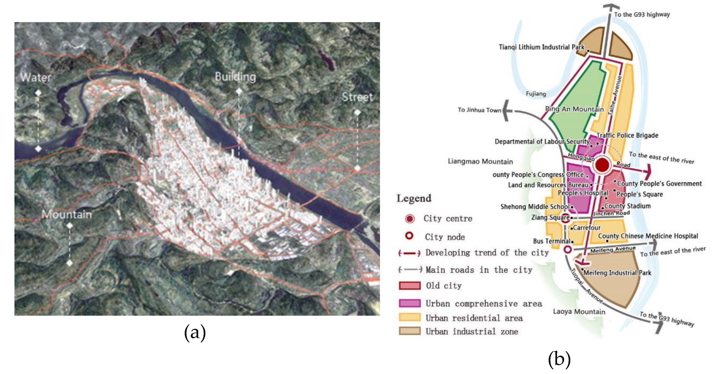
The city is a typical monocentric small city with one city center (red spot in Figure 3b), located at the old town center. Limited by hilly terrain and the Fujiang River, the city’s development took place mainly in two directions: north and south (Figure 3). The old town center was converted into a new high-density city center with mixed commercial and residential land use. However, its original street structure remained untouched, although there were some minor renovations. The leading industries are wineries and aluminum–magnesium manufacturing. Two industrial development clusters are located in the south and the north at the two ends of Taihe Avenue.

2.2. Data and Preprocessing

2.2.1. Data

The data used in this paper include Baidu heat map data, POI data, urban land use data, and building data for Shehong County. Among them, Baidu heat map data were collected from a Baidu map using Python programming language. POI data were collected from a Baidu map using the LocoySpider 8.5 web crawler software.
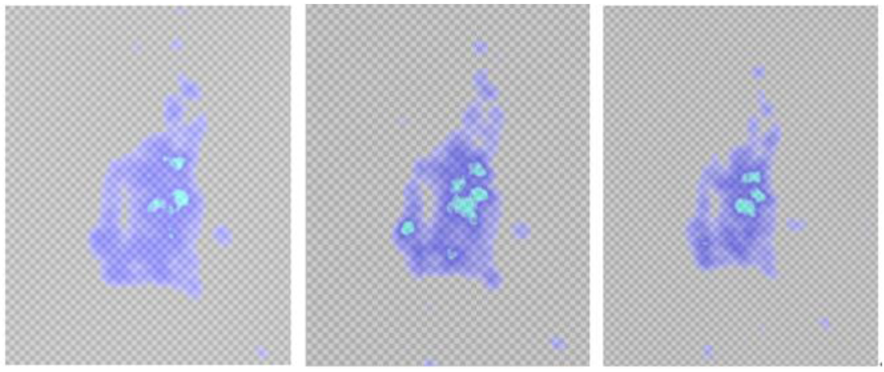
A Baidu heat map is a big data visualization product launched by Baidu in 2014. When a person uses some mobile APPs, the software provider obtains the user’s geographic location, provided that the user has agreed to their data collection policy. In such a way, Baidu collects user tracking data and provides or exchanges these data to its cooperating companies (Figure 4) [46]. Based on the geographical data of hundreds of millions of mobile phone users on their LBS platform, a Baidu heat map shows the changes in population aggregation in successive time spans and different regions based on Baidu users’ location information [14]. We collected Baidu heat map data for a weekday and a weekend day. For each day, data were collected at an interval of 1 h from 7:00 a.m. to 11:00 p.m. In total, 34 groups were collected (Figure 5).
In a geographic information system, a POI may be a building, a shop, a station, a road, and so forth [47]. We collected 6735 POIs for Shehong County from a Baidu map in 2018. The POI data were in tabular format, which included the Baidu coordinates, addresses, and names of the POIs.
The land use data were divided into 8 categories and 35 subcategories according to the “Code for classification of urban land use and planning standards of development land” (GB 50137–2011). Building data included the outlines and floors of all buildings, which were collected from local agencies.

2.2.2. Data Preprocessing

The land use and building data were AutoCAD format files. We converted them into shape files using ESRI ArcGIS software tools, as shown in Figure 6. The WGS_1984_UTM_Zone_48N coordinate system was used as the default coordinate system in this paper. The crawled Baidu heat map data had no coordinate system, so they were converted into the WGS_1984_UTM_Zone_48N coordinate system using the georeferencing tool in ESRI ArcGIS. In a Baidu heat map, the value of the pixel indicates the magnitude of the population aggregation. The grid score of a Baidu heat map image is used to represent population aggregation in successive analyses.
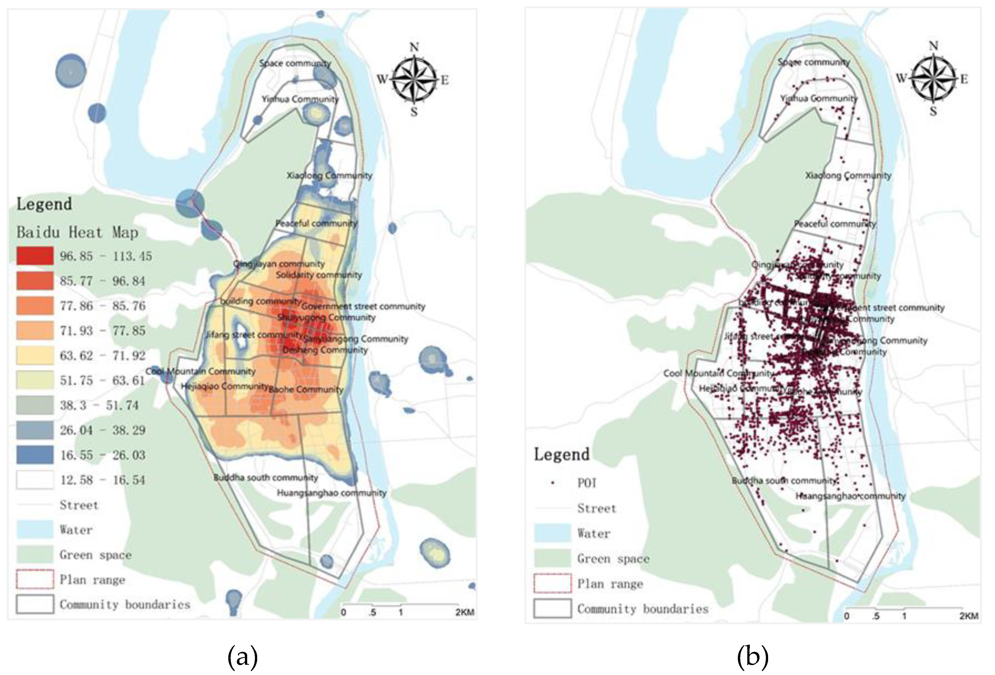
The POI data in the Baidu coordinate system were converted into the WGS_1984_UTM_Zone_48N coordinate system by the universal coordinate converter and ESRI ArcGIS conversion and projection tool. Final Baidu heat map, POI, land use, and building data are shown in Figure 7.

2.3. Methods

2.3.1. Getis–Ord general G

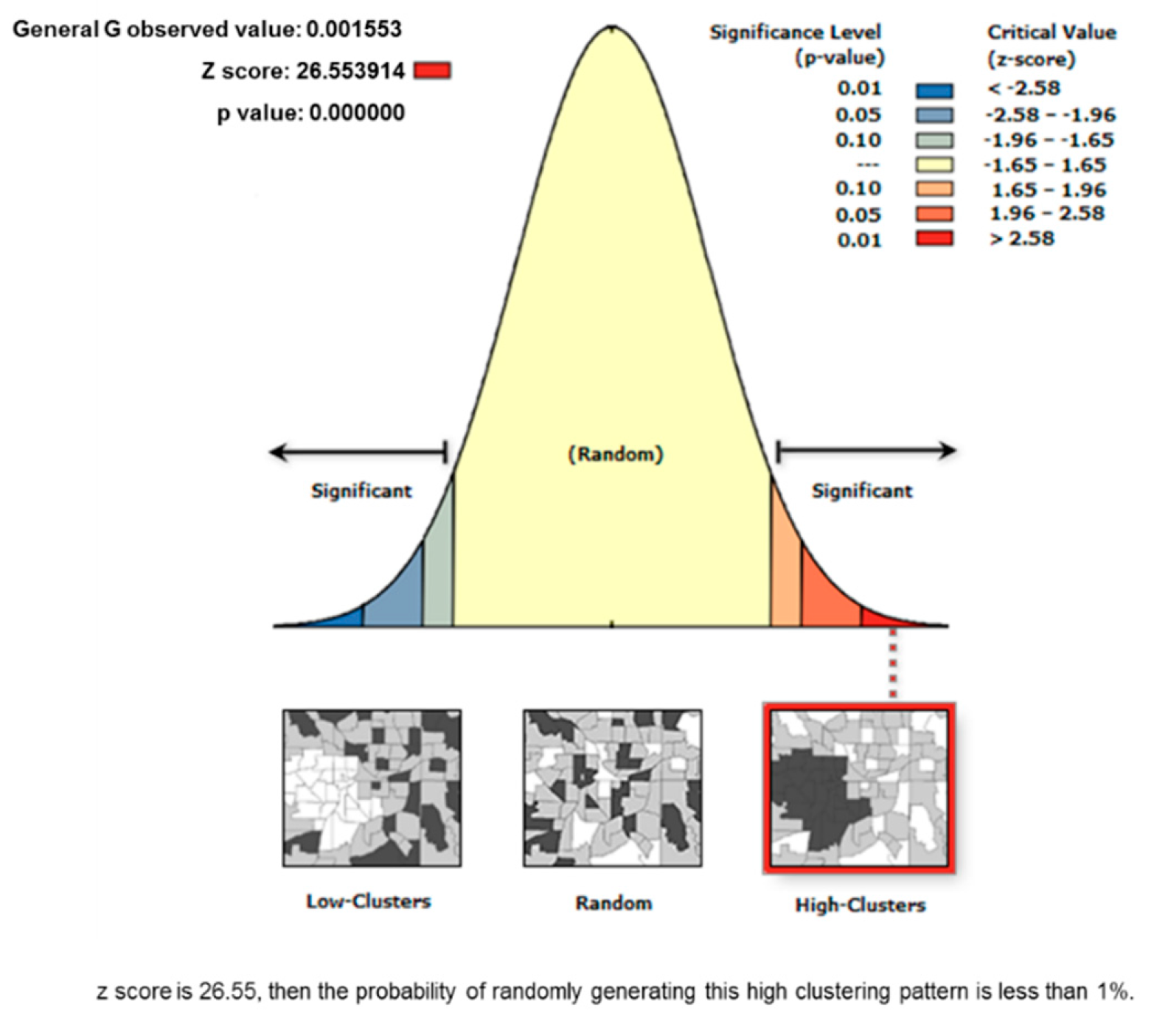
The distribution of features in space can be divided into aggregation, discrete, and random patterns (Figure 8) [48]. The degree of agglomeration can be judged according to the spatial correlation. There are many spatial correlation analysis methods, among which the Getis–Ord general G method is suitable for analyzing population agglomeration of Baidu heat maps. Using the pixel values of Baidu heat maps to discuss population aggregation degree may result in high-value pixel aggregation (representing high-density human aggregation trends) or low-value pixel aggregation (low-density human aggregation trends). In the Getis–Ord general G, z-scores are positive for high-density human aggregation and negative for low-density human aggregation [48].
The equation of Getis–Ord general G can be expressed as [48]
G = i = 1 n j = 1 n w i , j x i x j i = 1 n j = 1 n x i x j ,   j i
where x i and x j are attribute values for features i and j, respectively, w i , j is the spatial weight between features i and j, n is the number of features in the dataset, and j i .
The ZG-score for the statistic was computed as
Z G = G E ( G ) V ( G )
where
E [ G ] = i = 1 n j = 1 n w i , j n ( n 1 ) ,   j i
V [ G ] = E [ G 2 ] E [ G ] 2 .
In the above equation, the only difference between the numerator and the denominator is the weight ( w i , j ). Getis–Ord general G only handles positive values. Therefore, if the weight is binary (0/1) or always less than 1, the range of general G will be between 0 and 1.
Five scores can be obtained using the Getis–Ord general G tool in ESRI ArcGIS: general G observations, general G expectations, variance, z-scores, and p-values (Figure 9). In the ESRI ArcGIS [48], Getis–Ord general G is an inferential statistic, so the result must be interpreted under the null hypothesis. If the p-value returned by this method is small and statistically significant, the null hypothesis can be rejected. If the null hypothesis is rejected, the sign of the z-score will become very important. If the z-score is positive, the observed general G index will be larger than the expected general G index, indicating that the high value of the attribute will be clustered in the study area. The larger the z-score, the higher aggregation of the high value. If the z-score is negative, the observed general G index will be smaller than the expected general G index, indicating that the low value of the attribute will be clustered in the study area. The lower the value agglomeration, the higher the aggregation degree. If the z-score is close to zero, there is no obvious aggregation within the study area.
Baidu heat map data indicate the high and low densities of population aggregation by the high and low pixel values. Using the pixel value of a Baidu heat map to discuss the degree of aggregation may result in high-value pixel aggregation (high-density population aggregation trends) or low-value cell aggregation (low-density population aggregation trend). When the p-value is statistically significant, the high/low aggregation analysis can distinguish whether the space is high- or low-value agglomeration according to the z-score being positive or negative (when the z-score is positive, the space is high-value agglomeration; when the z-score is negative, the space is low-value aggregation).
Based on the general understanding of the pattern of crowd activities in a city, the activities of the citizens manifest a cyclical pattern on a weekly basis. The distributions of people on weekends (Saturday and Sunday) and weekdays (Monday–Friday) show particular differences [14,49]. Therefore, we selected a weekday and a weekend day with similar weather to examine the variation characteristics of the population aggregation pattern in Shehong County.

2.3.2. Raster Data Overlay

A Baidu heat map represents dynamic time data. To analyze the total population aggregation in a certain period of time in the city, we needed to overlay all the Baidu heat maps in the time period and then find the average to obtain the distribution of people aggregation in this time period. The equation used is as follows:
H I = i = 1 n h i / n
where HI denotes the average population aggregation degree in the I time period; hi represents the aggregate degree at time i in the I time period, such as 7:00, 8:00, and 11:00 a.m.; and n represents the number of times a Baidu heat map was collected during the I time period. For example, if a Baidu heat map were collected every hour to find the average aggregation degree of a certain city within 24 h, then n = 24.
We used Equation (5) to calculate the heat map of all workdays and weekends in Shehong County and used the natural break method to classify the calculated pixel values into 10 categories, for which the higher the value, the greater the aggregation degree.

2.3.3. Chi-Squared and Pearson Correlation Coefficient Tests

In order to reveal the relationship between people aggregation and land use, we analyzed correlations and significances between population aggregation degree and parcel attributes. Among them, the population aggregation degree was represented by the average population aggregation degree during the main activity time of the working day (7:00 a.m. to 11:00 p.m.), which reflected the overall situation of the population aggregation at the main activity time. Land parcel attributes include land type, POI density, floor area ratio, building density, land area, and so on. In addition, different land parcel division methods may affect the correlations between population aggregation degree and land parcels, so we divided the land parcels into three dimensions: land use parcel, road network blocks, and grids (Figure 10). We used ESRI ArcGIS to extract people aggregation and land parcel attributes and then performed data correlation analysis in IBM SPSS.
The Baidu heat score of the population aggregation degree is a quantitative variable, and the land type is a categorical variable, so the correlations between them should be calculated by a chi-squared test, Pearson x2. The equation is [50]
x 2 =   ( A E ) 2 E = i = 1 k ( A i E i ) 2 E i = i = 1 k ( A i n p i ) 2 n p i   ( i = 1 ,   2 , 3 , , k )
where A i is the observation frequency of the i level, E i is the desired frequency of the i level, n is the total frequency, and p i is the desired frequency of the i level. The expected frequency E i of the i level is equal to the expected probability p i of the total frequency n × i level, and k is the number of cells. When n is relatively large, the x 2 statistic approximates the chi-squared distribution of k-1 (the number of parameters used in calculating E i ) degrees of freedom.
Because parcel attributes such as POI density, floor area ratio, building density, and land area are all continuous variables, the correlations between the population aggregation and parcel attributes can be tested by the Pearson correlation coefficient tests. The Pearson correlation coefficient between two variables is defined as the quotient of the covariance and standard deviation between the two variables:
ρ X , Y = cov ( X , Y ) σ X σ Y = E [ ( X μ X ) ( Y μ Y ) ] σ X σ Y .
The Pearson correlation coefficient varies from −1 to 1. In the behavioral sciences [51], 0.00 ≤ |r| ≤ 0.09 indicates no correlation, 0.1 ≤ |r| ≤ 0.3 indicates a weak correlation, 0.3 < |r| ≤ 0.5 indicates a medium correlation, and 0.5 < |r| ≤1 indicates a strong correlation.

3. Results

3.1. Temporal Characteristics of Population Aggregation

To analyze the temporal characteristics of the population aggregation pattern in Shehong County, the z-scores of all time slots for the two days were represented by lines and the time variance of aggregation for two days were obtained (Figure 11).

3.1.1. Workday

On the workday, at the 0.01 significance level, the z-score of the Getis–Ord general G was between 18.16 and 31.72, which means that the aggregation of the population in Shehong County was clustered into a high-value gathering trend on the workday; that is, a high-density people concentration had a tendency to gather. The z-score at 7:00 a.m. was 18.16, which was lower than the other times on the same day, indicating that the distribution of the population in Shehong County was more dispersed than at other times. By 8:00–9:00 a.m., the z-score rose rapidly and reached a peak, which was coordinated with the morning commuting time. From this, the following inferences can be made: in the morning, as people move from home to work place, the population aggregation degree quickly increased and reached the first peak of clustering of the working day. At 10:00–11:00 a.m., the population aggregation degree was in a stable state and then gradually declined, forming a trough at 1:00 p.m. Since 1:00 p.m. is a lunch break, some people may return to their homes to rest at noon, resulting in a decrease in the population aggregation degree. At 2:00 and 4:00 p.m., there were two population aggregation peaks. The population aggregation degree was reduced around 6:00 p.m., which is consistent with off-hours.

3.1.2. Weekend

At the 0.01 significance level, the z-score of the Getis–Ord general G on the weekend was between 17.50 and 28.56, which means that a high-density people concentration had a tendency to gather on the weekend. We found that 7:00 a.m. was the lowest for the population aggregation degree. After 7:00 a.m., the population aggregation degree gradually increased, and two gentle peaks occurred at 11:00 a.m. and 12:00 p.m. From then until 5:00 p.m., the population aggregation degree was relatively stable and gradually decreased at 6:00 p.m. However, there was still a high degree of population aggregation around 10:00 p.m.

3.1.3. Comparison of the Workday and the Weekend

Comparing the temporal characteristics of the population aggregation on the workday and weekend day of Shehong County (Figure 11), we found the following:
(1) On both the weekday and weekend, the population aggregation degree of the daytime was greater than that at night based on z-scores. This is consistent with common sense, that people in residential areas have a lower aggregation degree than public activities [14], thus providing the facial validity of our results.
(2) Regarding the population aggregation degree, the z-scores indicate that people on the workday are more clustered than on the weekend before 10:00 p.m., but the aggregation trends reverse after 10:00 p.m., when the weekend is more clustered than the workday.
(3) On the volatility of the population aggregation, by comparing the fluctuations of the curve of the population aggregation, volatility for most time periods of the weekday was greater than on the weekend. Comparing the curvature of the morning and afternoon curves, on the weekday, people gathered and dispersed faster than on the weekend.

3.2. Spatial Distribution Characteristics of Population Aggregation

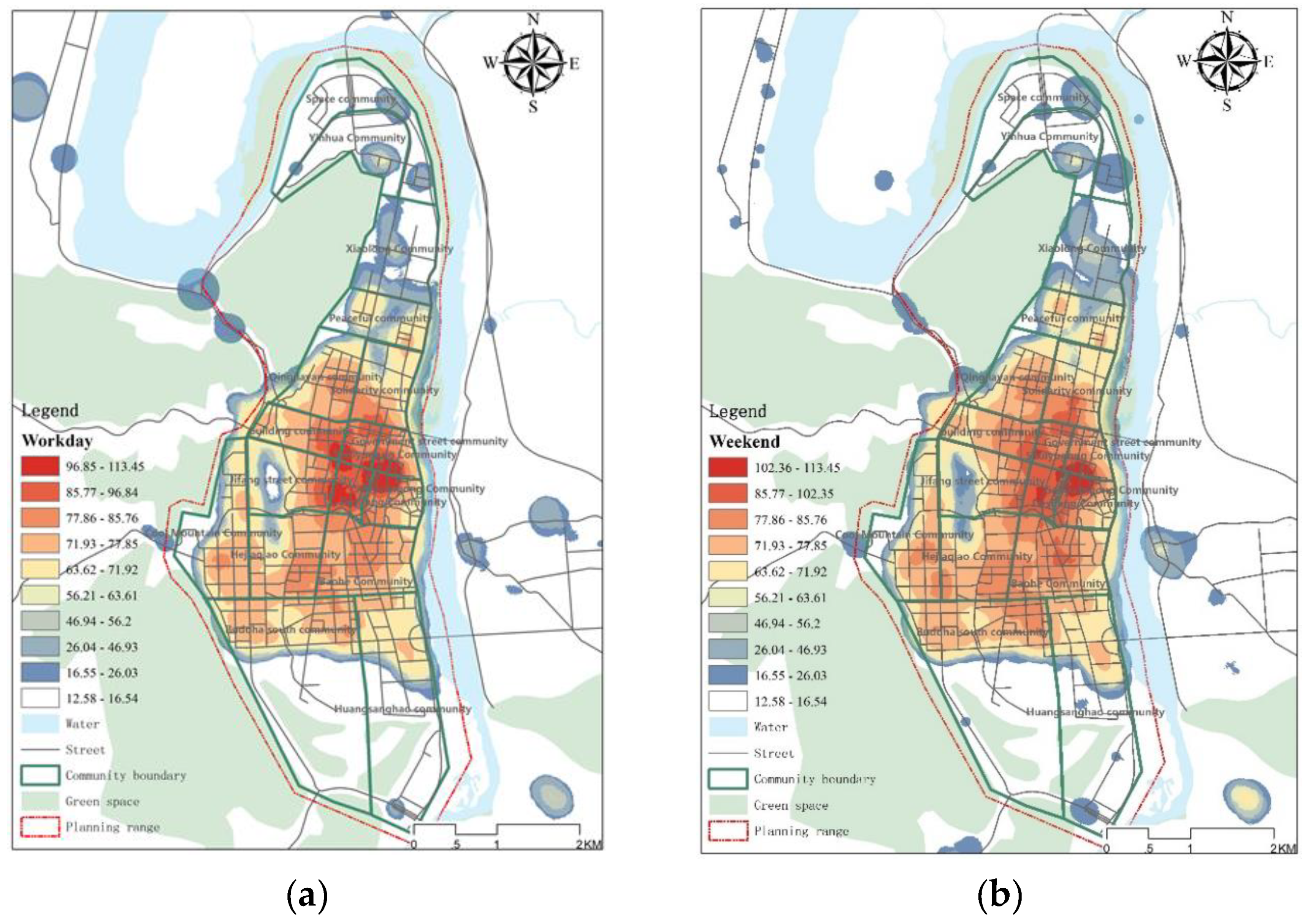
We used Equation (5) to count all heat maps of the working day and weekend. Then, we used the natural break method to divide the calculation results into 10 categories according to the pixel score. Cold and warm colors were used to indicate the degree of population aggregation; a warmer color represents a higher clustering of people. The spatial distribution characteristics of the population aggregation on the workday and weekend in Shehong County are shown in Figure.

3.2.1. Workday

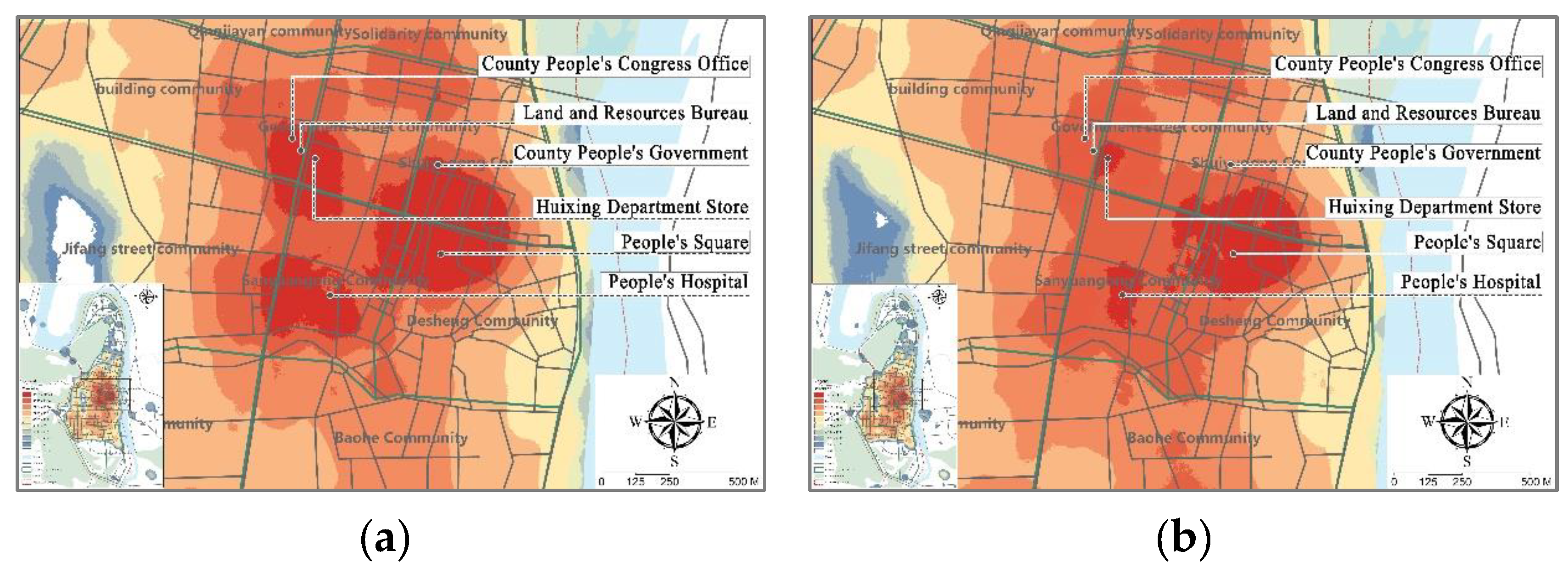
It can be seen from (a) of Figure 12 and (a) of Figure 13 that there are mainly three high aggregation areas in the Shehong County on the workday, they are People’s Square, People’s Hospital and Land Resources Bureau. The People’s Square is the main public activity venue for people of Shehong County. The northern part of People’s Square is where the county’s government buildings are located. People’s Square is surrounded by commercial buildings, such as the New Century Commercial Plaza and the Yongjia Supermarket. There are also public service buildings, such as government buildings, information service centers, and so on. Therefore, the population aggregation near the People’s Square has large numbers of working and shopping people. The People’s Hospital is located in the east of Taihe Avenue, south of Guanghan Road, and there are no large commercial buildings or other public service buildings nearby. The Land Resources Bureau is located in the west of the middle section of Taihe Avenue, south of Democratic Lane, surrounded by public service buildings, such as the county people’s congress, the county land transaction and service center, and the county employment service bureau. In general, the people in Shehong County gather together for work, leisure shopping, and medical treatment on weekdays.

3.2.2. Weekend

It can be seen from Figure 12b and Figure 13b that there are also three high-aggregation areas in Shehong County on the weekend: the People’s Square, the People’s Hospital, and the Land Resources Bureau. Compared with the workday, it was found that the area of the high-aggregation area was much smaller than the weekend. Moreover, the high-aggregation area of the Land Resources Bureau was reduced compared with the Huixing Department Store in the southeast and another in the southern business district.

3.2.3. Comparison of the Workday and the Weekend

By comparing the spatial characteristics of the population aggregation on the workday and weekend in Shehong County, we found the following:
(1) The locations of population aggregation in Shehong County have a high degree of overlap on the workday and weekend. This is different from the conclusion reached for Shanghai: “On the workday and weekend, there is a big difference in the population aggregation in downtown Shanghai (the workday is mainly concentrated in the Century Avenue, Lujiazui, Jing’an Temple, Shanghai Railway Station, etc. The weekend is mainly concentrated in People’s Square, Xujiahui, Zhongshan. Park, Jinshajiang Road Subway Station, etc.)” [14].
(2) The workday has larger high population aggregation areas than the weekend. This shows that people on the workday are more clustered than on weekend, which is consistent with the conclusion drawn in Section 3.1.3.

3.3. Correlation between Population Aggregation and Land Parcel attributes

3.3.1. Analysis Results Based on the Land Use Parcels

The land parcel attributes we extracted were land type, POI density, floor area ratio, building density, and land area. The Baidu heat score of the population aggregation degree is a quantitative variable, and the land type is a categorical variable, so the correlations between them should be calculated by a chi-squared test. Because parcel attributes such as POI density, floor area ratio, building density, and land area are all continuous variables, the correlations between the population aggregation and parcel attributes can be tested by the Pearson correlations coefficient tests.
(1) Correlation between Population Aggregation and Parcel Type.
The correlation between population aggregation and land parcel type was analyzed by a chi-squared test using SPSS. The results are shown as Table 1.
Progressive significance tests between population aggregation and land parcel type revealed no evidence of a relationship between the population aggregation and the parcel type. The reason for this result could be that population aggregation is not only affected by the land type but also by other factors, such as the density of POI, development time, and mode. For example, the population aggregation of the residential land in the old city center was generally higher than that of the newly developed residential land in suburbs. At the same location and under the same development time, the population aggregation in the higher floor area ratio was higher than that of the lower floor area ratio.
(2) Correlations between Population Aggregation and POI Density, Floor Area Ratio, Building Density, and Land Area.
We used the Pearson correlation coefficient in SPSS to explore the relationship between the degree of population aggregation and land parcel attributes, which were POI density, building density, floor area ratio, and land area. The results are shown in Table 2. The p-values of the significance of correlations between population aggregation degree and the POI density, the floor area ratio, the building density, and the land area were less than or equal to 0.01(indicated by two asterisks), indicating that the null hypothesis was rejected. Among them, the population aggregation degree was positively correlated with the POI density, floor area ratio, and building density. The population aggregation degree was negatively correlated with the land parcel area.

3.3.2. Analysis Results Based on the Road Network Blocks

For the road network blocks, the land parcel attributes we extracted included POI density, floor area ratio, building density, and land area. A land parcel may contain multiple types of road network blocks, so land type was no longer used as an attribute of road network blocks. The results of the correlation analysis between the population aggregation degree and the abovementioned land parcel attributes are shown in the Table 3. It can be seen that at a significance level of 0.01, the correlations between population aggregation degree and POI density, floor area ratio, building density, and land area were significant. The population aggregation degree positively correlated with POI density, floor area ratio, and building density and negatively correlated with land area.

3.3.3. Analysis Results Based on Grids

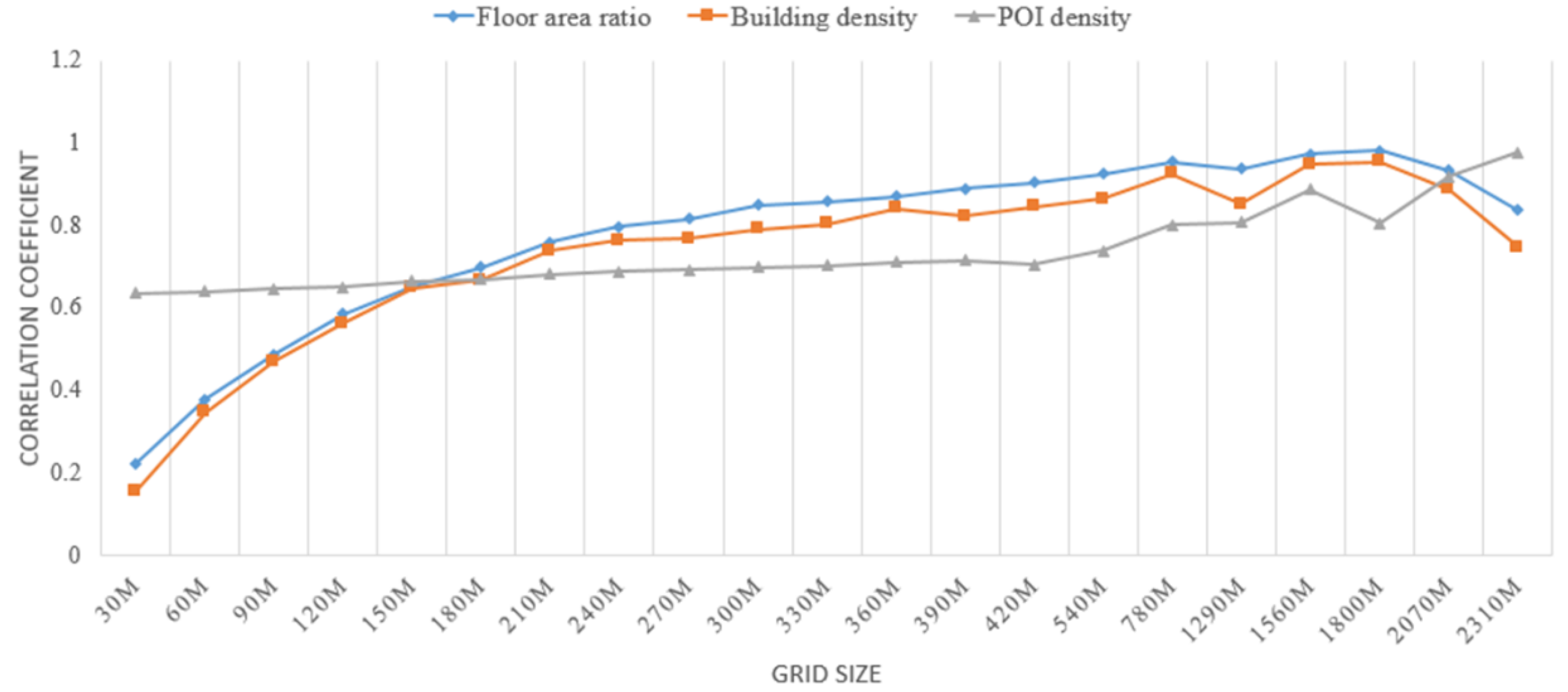
For the regular grid scale, the land parcel attributes we extracted included POI density, floor area ratio, and building density. The land area of each regular grid was the same, and one grid cell may contain multiple land use types, so land type and land area were no longer used as land parcel attributes. Starting from a 30 m by 30 m grid, we gradually increased the grid size at a 30m interval to form multiple scale sequences. The number of grid cells dropped from 11605 (30 m) to 8 (2310 m). The correlation analysis results of the population aggregation degree and the attributes in each grid size are shown in Appendix A. It can be seen that at a significance level of 0.01, the correlations between population aggregation degree and POI density, floor area ratio, and building density were significant, and they were positively correlated. For the correlation coefficient, the correlation coefficient between population aggregation degree and POI density, floor area ratio, and building density increased with the increase of the grid size, and the correlation coefficient reached the maximum at 1800 × 1800 m (Figure 14). Prior to the 420 × 420 m grid, the correlation coefficient between population aggregation degree and POI density increased slowly. After that, the growth was faster, and the grid reached a maximum at the test boundary of 2310 × 2310 m.

4. Discussion

Our findings show that the weekday aggregation of people in Shehong County is higher than on the weekend, which is unlike the results for Shanghai: “The crowd tends to gather at a high intensity in a few centers during the weekend, while the crowd tends to gather at more centers on weekday, but the intensity of the agglomeration is relatively low” [14]. We speculate that there are two main reasons for this difference: Firstly, the land use pattern of the two cities are different. There is only one main working center in Shehong County, which is located in the center of the city, resulting in a higher concentration of people on the weekday. However, there are several major work areas in Shanghai, which leads to a lower concentration of people on the weekday than on the weekend. Secondly, cities have different attractions for their residents and the population of their vicinity. Shehong is a small city and its attraction is low on the weekend, while Shanghai, as a megacity, has more attractive destinations for weekends.
On the weekday and the weekend, the population aggregation in Shehong County has a high degree of overlap, which is different from the research results of Wuhan City: “Workdays and weekends, people clustered with great differences” [17]. We speculate that this difference may due to different urban structures. Wuhan is a multicenter megacity, and there is a clear boundary between the work areas and the entertainment areas, which leads to a large difference in the population aggregation on the weekday and the weekend. However, Shehong County, as a small city with a single center, has no clear boundary between the work and recreation areas. They are located in the same city center, which leads to a large overlap of the population aggregation on the weekday and the weekend.
To examine the influence of parcel division on the correlation between population aggregation degree and land parcel attributes, we divided the land parcels three different ways: land use parcel, road network blocks, and grids. We found that the correlation significance of the three divisions were unaffected by division methods. At a significance level of 0.01, the correlations between population aggregation degree and POI density, floor area ratio, and building density were significant and positively correlated. This shows that the division of land parcel method has little influence on judging whether population aggregation degree and POI density, floor area ratio, and building density are related or not. However, the division of land parcel method has an effect on the correlation coefficient. Using regular grid division, the correlation coefficient between population aggregation degree and POI density, floor area ratio, and building density will become larger when the grid size becomes larger.
Finally, when dividing the area by land use parcel, we found that the population aggregation degree is not significantly related to the land type, and this result is different from people’s common sense and deserves some further investigation since this assumption is used in some travel demand modeling processes.

5. Conclusions

Based on Baidu heat maps, we used Getis–Ord general G to obtain variations in the population aggregation on weekdays and the weekend in Shehong County. (1) On weekdays, the population aggregation of Shehong County is significantly higher than the weekend, and the peak of the aggregation is at 2:00 a.m. and 4:00 p.m. (2) People on weekdays gather with more volatility than on the weekend. People on weekdays gather and disperse at a significantly faster rate than on the weekend. (3) Regarding the aggregation position, the high aggregation area is where there is a concentration of business districts, administrative offices, people’s hospitals, and the People’s Square in the city center, on weekdays and the weekend. Population aggregation has a high degree of overlap in geographical locations in Shehong County.
Using the chi-squared test, we found that the correlation between the population aggregation and the land use was not significant. Through the Pearson correlation coefficient, we found that population aggregation degree and POI density, floor area ratio, and building density were significantly positively correlated, and the correlation coefficient increased as the mesh unit size increased. In the grid of 1800×1800m, the correlation coefficients between population aggregation degree and floor area ratio and building density reached the peak.
The results show that Baidu heat map data can reveal urban residents’ spatiotemporal aggregation pattern and the relationship between people aggregation and urban infrastructural settings. It may play an important role in urban and transportation planning by being treated as a supplementary data source to traditional urban planning data. This is especially the case when the costly and time-consuming full-scale traditional transportation OD (Origin-Destination) survey cannot be conducted due to manpower and finance constraints. Baidu heat maps can provide some coarse information about the origins and destinations of city residents’ trips at different times of day. Combined with traditional OD data or GPS tracking data, from which OD information can be derived, it can be used for travel demand analysis. Furthermore, Baidu heat maps can be used to find the mismatch between residents’ demand and urban infrastructure supplies. Baidu heat maps that represent people aggregation and POI data (educational points and administrative points in particular) that partly represent urban infrastructure can be examined by correlation analysis, and areas with weak correlations and high POI densities may indicate an insufficient usage of infrastructure. Finally, the people’s time-dependent spatial aggregation patterns may help city administrators with dynamic traffic management, which may effectively remedy traffic jam situations by applying different policies on weekends and workdays.
Although Baidu heat maps represent a huge number of Baidu users, it is still a biased sample from the total population; thus, it cannot simply be marked as a “real” population aggregation pattern. Further studies may investigate the following two aspects: (1) exploring the population aggregation in various functional areas of the city through POI data and Baidu heat maps; (2) cross-validating the relationship between population aggregation and land parcel attributes with multiple data sources, such as taxi GPS logs and mobile tracking logs.

Author Contributions

Conceptualization, D.F.; data curation, L.T.; formal analysis, Z.S.; investigation, D.F. and L.T.; methodology, D.F. and Z.S.; project administration, Z.S.; validation, L.T.; visualization, D.F.; writing—original draft, D.F. and L.T.; writing—review and editing, Z.S.

Funding

This research was funded by the National Key R&D Program of China, grant number 2018YFD1100304.

Conflicts of Interest

The authors declare no conflict of interest.

Appendix A

Table A1. Correlation analysis between people aggregation degree and POI density, floor area ratio, and building density on grids of different scales.
POI DensityFloor Area RatioBuilding Density
30×30 m GridPeople aggregation degree0.636 **0.0225 **0.157 **
Number of cases116051160511605
60 × 60 m GridPeople aggregation degree0.641 **0.379 **0.348 **
Number of cases358435843584
90 × 90 m GridPeople aggregation degree0.647 **0.489 **0.471 **
Number of cases176217621762
120 × 120 m GridPeople aggregation degree0.652 **0.586 **0.564 **
Number of cases106010601060
150 × 150 m GridPeople aggregation degree0.665 **0.654 **0.649 **
Number of cases733733733
180 × 180 m GridPeople aggregation degree0.670 **0.699 **0.668 **
Number of cases524524524
210 × 210 m GridPeople aggregation degree0.682 **0.760 **0.738 **
Number of cases410410410
240 × 240 m GridPeople aggregation degree0.688 **0.797 **0.765 **
Number of cases327327327
270 × 270 m GridPeople aggregation degree0.693 **0.817 **0.768 **
Number of cases264264264
300 × 300 m GridPeople aggregation degree0.700 **0.850 **0.792 **
Number of cases220220220
330 × 330 m GridPeople aggregation degree0.704 **0.859 **0.804 **
Number of cases190190190
360 × 360 m GridPeople aggregation degree0.712 **0.870 **0.842 **
Number of cases155155155
390 × 390 m GridPeople aggregation degree0.717 **0.889 **0.823 **
Number of cases143143143
420 × 420 m GridPeople aggregation degree0.705 **0.904 **0.845 **
Number of cases127127127
540 × 540 m GridPeople aggregation degree0.740 **0.926 **0.865 **
Number of cases787878
780 × 780 m GridPeople aggregation degree0.801 **0.955 **0.926 **
Number of cases484848
1290 × 1290 m GridPeople aggregation degree0.808 **0.937 **0.853 **
Number of cases202020
1560 × 1560 m GridPeople aggregation degree0.887 **0.974 **0.949 **
Number of cases161616
1800 × 1800 m GridPeople aggregation degree0.806 **0.981 **0.954 **
Number of cases101010
2070 × 2070 m GridPeople aggregation degree0.918 **0.934 **0.888 **
Number of cases101010
2310 × 2310 m GridPeople aggregation degree0.978 **0.837 **0.747 **
Number of cases888
**: Correlation is significant when the confidence (two sides) is 0.01; *: Correlation is significant when the confidence (two sides) is 0.05.

References

  1. Zhou, J.; Hou, Q.; Dong, W. Spatial Characteristics of Population Activities in Suburban Villages Based on Cellphone Signaling Analysis. Sustainability 2019, 11, 2159. [Google Scholar] [CrossRef]
  2. Sun, C.; Luo, Y.; Li, J. Urban traffic infrastructure investment and air pollution: Evidence from the 83 cities in China. J. Clean. Prod. 2018, 172, 488–496. [Google Scholar] [CrossRef]
  3. Sciences, C.A.O.T.; Cloud, A. 2017 Traffic Analysis Reports for Major Cities in China. Available online: http://www.cnki.com.cn/Article/CJFDTotal-CSCL201803004.htm (accessed on 26 October 2019).
  4. J, D.; Wang, Y.; Wang, L.; Chen, L.; Hu, B.; Tang, G.; Xin, J.; Song, T.; Wen, T.; Sun, Y.; et al. Analysis of heavy pollution episodes in selected cities of northern China. Atmos. Environ. 2012, 50, 338–348. [Google Scholar] [CrossRef]
  5. Ma, L.; Li, D.; Tao, X.; Dong, H.; He, B.; Ye, X. Inequality, Bi-Polarization and Mobility of Urban Infrastructure Investment in China’s Urban System. Sustainability 2017, 9, 1600. [Google Scholar] [CrossRef]
  6. Alfonso Piña, H.W.; Pardo Martínez, I.C. Development and Urban Sustainability: An Analysis of Efficiency Using Data Envelopment Analysis. Sustainability 2016, 8, 148. [Google Scholar] [CrossRef]
  7. Ma, X.; Wu, Y.-J.; Wang, Y.; Chen, F.; Liu, J. Mining smart card data for transit riders’ travel patterns. Transp. Res. Part C Emerg. Technol. 2013, 36, 1–12. [Google Scholar] [CrossRef]
  8. Kim, M.-K.; Kim, S.; Sohn, H.-G. Relationship between spatio-temporal travel patterns derived from smart-card data and local environmental characteristics of Seoul, Korea. Sustainability 2018, 10, 787. [Google Scholar]
  9. Goulet-Langlois, G.; Koutsopoulos, H.N.; Zhao, J. Inferring patterns in the multi-week activity sequences of public transport users. Transp. Res. Part C Emerg. Technol. 2016, 64, 1–16. [Google Scholar] [CrossRef] [Green Version]
  10. Gonzalez, M.C.; Hidalgo, C.A.; Barabasi, A.-L. Understanding individual human mobility patterns. Nature 2008, 453, 779. [Google Scholar] [CrossRef]
  11. Ahas, R.; Aasa, A.; Silm, S.; Tiru, M. Daily rhythms of suburban commuters’ movements in the Tallinn metropolitan area: Case study with mobile positioning data. Transp. Res. Part C Emerg. Technol. 2010, 18, 45–54. [Google Scholar] [CrossRef]
  12. Calabrese, F.; Diao, M.; Di Lorenzo, G.; Ferreira, J., Jr.; Ratti, C. Understanding individual mobility patterns from urban sensing data: A mobile phone trace example. Transp. Res. Part C Emerg. Technol. 2013, 26, 301–313. [Google Scholar] [CrossRef]
  13. Hoteit, S.; Secci, S.; Sobolevsky, S.; Pujolle, G.; Ratti, C. Estimating real human trajectories through mobile phone data. In Proceedings of the 2013 IEEE 14th International Conference on Mobile Data Management, Milan, Italy, 3–6 June 2013; pp. 148–153. [Google Scholar]
  14. Wu, Z.Q.; Ye, Z.N. Research on urban spatial structure based on Baidu heat map: A study on the central city of Shanghai. City Plan. Rev. 2016, 40, 33–40. [Google Scholar]
  15. He, S.; Hang, D.; Zhang, M. Research on dynamic changes of urban square space in spatial and temporal based on Baidu thermal diagram a case study on the Wuyi square of Changsha. In Proceedings of the IEEE 2nd International Conference on Big Data Analysis, Beijing, China, 10–12 March 2017. [Google Scholar]
  16. Jianwei, X.; Yuanfei, Z.; Tianle, Q.; Yan, L. Evaluation of downtown spatial characteristics of Nanchang. Planners 2018, 34, 120–125. [Google Scholar]
  17. Lucang, W. Spatial-temporal characteristics of urban population aggregation based on baidu heat map in central areas of Wuhan city. J. Hum. Settl. West China 2018, 33, 52–56. [Google Scholar]
  18. Reades, J.; Calabrese, F.; Ratti, C. Eigenplaces: Analysing cities using the space–time structure of the mobile phone network. Environ. Plan. B Plan. Des. 2009, 36, 824–836. [Google Scholar] [CrossRef]
  19. Ahas, R.; Aasa, A.; Mark, Ü.; Pae, T.; Kull, A. Seasonal tourism spaces in Estonia: Case study with mobile positioning data. Tour. Manag. 2007, 28, 898–910. [Google Scholar] [CrossRef]
  20. Zhang, K.; Wang, M.; Wei, B.; Sun, D.J. Identification and prediction of large pedestrian flow in urban areas based on a hybrid detection approach. Sustainability 2017, 9, 36. [Google Scholar] [CrossRef]
  21. Langford, M. An evaluation of small area population estimation techniques using open access ancillary data. Geogr. Anal. 2013, 45, 324–344. [Google Scholar] [CrossRef]
  22. Thom, D.; Bosch, H.; Koch, S.; Wörner, M.; Ertl, T. Spatiotemporal Anomaly Detection through Visual Analysis of Geolocated Twitter Messages. In Proceedings of the IEEE Pacific Visualization Symposium, Songdo, Korea, 8 Feburay–2 March 2012. [Google Scholar]
  23. Li, J.; Ying, L.; Dang, A. Live-Work-Play Centers of Chinese cities: Identification and temporal evolution with emerging data. Comput. Environ. Urban Syst. 2018, 71, 58–66. [Google Scholar] [CrossRef]
  24. Zhongnan, Y.; Yihui, C. Quantitative study on space use around urban rail transit station based on network data: A case of Shanghai metro line 10. Shanghai Urban Plan. Rev. 2017, 137, 122–128. [Google Scholar]
  25. Lin, L.; Difei, J. Research on The Classification Method of Historcial Streets Based on Big Data. Chin. Overseas Archit. 2016, 8, 17. [Google Scholar]
  26. Lihua, F.; Yaohui, P.; Zhenchun, M.; Mei, X.; Xingyan, G. Analysis on Distribution Characteristics of Business Community Center in Zhuzhou Based on Big Data. J. Nat. Sci. Hunan Norm. Univ. 2018, 41, 17–23. [Google Scholar]
  27. Bingrong, L.; Ying, Y.; Daquan, H.; Zheng, Y. Big data based job-residence relation in Chongqing metropolitan area. Planners 2015, 31, 92–96. [Google Scholar]
  28. Xin, T.; Daquan, H.; Xingshuo, Z. Research on the measurement of occupational residence balance based on Baidu heat map. J. Beijing Norm. Univ. 2016, 52, 622–627. [Google Scholar]
  29. Roth, C.; Kang, S.M.; Batty, M.; Barthélemy, M. Structure of urban movements: Polycentric activity and entangled hierarchical flows. PLoS ONE 2011, 6, e15923. [Google Scholar] [CrossRef] [PubMed]
  30. Pei, T.; Sobolevsky, S.; Ratti, C.; Shaw, S.-L.; Li, T.; Zhou, C. A new insight into land use classification based on aggregated mobile phone data. Int. J. Geogr. Inf. Sci. 2014, 28, 1988–2007. [Google Scholar] [CrossRef] [Green Version]
  31. Wang, C.; Huang, C.; Pengfei, L.I.; Wang, C. A Research on Spatio-temporal Characteristics and Motivation of Space Utilization in the Center District of City:A Case Study of Nanjing Xinjiekou Area. Mod. Urban Res. 2016, 7, 13. [Google Scholar]
  32. Kang, Y.; Wang, Y.; Xia, Z.; Jiao, C.; Jiao, L.; Wei, Z. Identification and Classification of Wuhan Urban Districts Based on POI. J. Geomat. 2018, 43, 81–85. [Google Scholar]
  33. Yao, Y.; Li, X.; Xiaoping, L.; Penghua, L.; Zhaotang, L.; Jinbao, Z.; Mai, K. Sensing spatial distribution of urban land use by integrating points-of-interest and Google Word2Vec model. Int. J. Geogr. Inf. Sci. 2016, 31, 825–848. [Google Scholar] [CrossRef]
  34. Xinyi, N.; Liang, D.; Xiaodong, S. Understanding Urban Spatial Structure of Shanghai Central City Based on Mobile Phone Data. China City Plan. Rev. 2015, 24, 15–23. [Google Scholar]
  35. Weijing, Z.; De, W. Urban space study based on the temporal characteristics of residents’ behavior. Prog. Geogr. 2018, 37, 1106–1118. [Google Scholar]
  36. Hao, M.; Rohrdantz, C.; Janetzko, H.; Dayal, U.; Hsu, M. Visual sentiment analysis on twitter data streams. In Proceedings of the IEEE Conference on Visual Analytics Science and Technology, Providence, RI, USA, 23–28 October 2011. [Google Scholar]
  37. Calabrese, F.; Colonna, M.; Lovisolo, P.; Parata, D.; Ratti, C. Real-time urban monitoring using cell phones: A case study in Rome. IEEE Trans. Intell. Transp. Syst. 2010, 12, 141–151. [Google Scholar] [CrossRef]
  38. Stepanyan, K.; Borau, K.; Ullrich, C. A Social Network Analysis Perspective on Student Interaction within the Twitter Microblogging Environment. In Proceedings of the 10th IEEE International Conference on Advanced Learning Technologies, Sousse, Tunisia, 5–7 July 2010. [Google Scholar]
  39. Mora, H.; Pérez-delHoyo, R.; Paredes-Pérez, J.; Mollá-Sirvent, R. Analysis of Social Networking Service Data for Smart Urban Planning. Sustainability 2018, 10, 4732. [Google Scholar] [CrossRef]
  40. Gerber, M.S. Predicting crime using Twitter and kernel density estimation. Decis. Support Syst. 2014, 61, 115–125. [Google Scholar] [CrossRef]
  41. Ke, C.; Jonikristian, K. Pedestrian Density Analysis in Public Scenes With Spatiotemporal Tensor Features. IEEE Trans. Intell. Transp. Syst. 2016, 17, 1968–1977. [Google Scholar]
  42. Tauno, M.; Jaak, V. ClustVis: A web tool for visualizing clustering of multivariate data using Principal Component Analysis and heatmap. Nucleic Acids Res. 2015, 43, W566–W570. [Google Scholar]
  43. Wang, W.-T.; Wu, Y.-L.; Tang, C.-Y.; Hor, M.-K. Adaptive density-based spatial clustering of applications with noise (DBSCAN) according to data. In Proceedings of the 2015 International Conference on Machine Learning and Cybernetics (ICMLC), Guangzhou, China, 12–15 July 2015; pp. 445–451. [Google Scholar]
  44. Jordi, D.; Schroeder, M.P.; Nuria, L. jHeatmap: An interactive heatmap viewer for the web. Bioinformatics 2014, 30, 1757–1758. [Google Scholar]
  45. Zhang, S.; Yang, R.; Zhao, Y. Coarse-Grained Parallel AP Clustering Algorithm based on Intra-Class and Inter-Class Distance. Int. J. Perform. Eng. 2018, 14, 3174–3183. [Google Scholar] [CrossRef]
  46. Baidu Map Open Platform: Intelligent Positioning. Available online: http://lbsyun.baidu.com/products/products/location (accessed on 22 October 2019).
  47. Han, G.; Yongpei, G.; Nana, C. Study on the population flow and population clusters in the sixth ring road of Beijing based on multivariate data. Urban Dev. Stud. 2018, 25, 107–112. [Google Scholar]
  48. ArcGIS Resources. Available online: http://resources.arcgis.com/en/help/main/10.2/ (accessed on 6 July 2019).
  49. Baohong, H.; Yan, H.; Yujia, W.; Xiang, Z. Selection Mechanisms of Residents’ Daily Activity-travel Behavior with Housing Mobility. J. Transp. Syst. Eng. Inf. Technol. 2017, 17, 19–25. [Google Scholar]
  50. Banker, R.D.; Morey, R.C. The Use of Categorical Variables in Data Envelopment Analysis. Manag. Sci. 1986, 32, 1613–1627. [Google Scholar] [CrossRef]
  51. Muller, K. Statistical Power Analysis for the Behavioral Sciences. Technometrics 1989, 31, 499–500. [Google Scholar] [CrossRef]
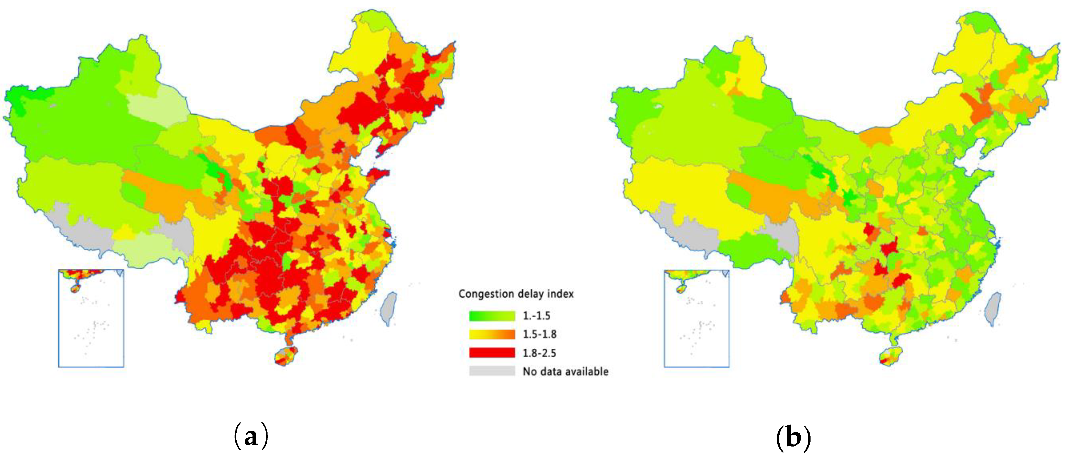
Figure 1. Chinese urban commuting congestion map: (a) peak periods and (b) ordinary periods [3].
Sustainability 11 06276 g001
Figure 2. Location of Shehong County.
Sustainability 11 06276 g002
Figure 3. Study area status: (a) aerial view of the study area map and (b) functional map.
Sustainability 11 06276 g003
Figure 4. A part of the mobile APP of Baidu location service [46].
Sustainability 11 06276 g004
Figure 5. Baidu heat map examples.
Sustainability 11 06276 g005
Figure 6. Building data in shape file format.
Sustainability 11 06276 g006
Figure 7. Preprocessed data: (a) preprocessed Baidu heat map data and (b) preprocessed point of interest (POI) data.
Sustainability 11 06276 g007
Figure 8. Feature aggregation pattern [48].
Sustainability 11 06276 g008
Figure 9. The result of Getis–Ord general G.
Sustainability 11 06276 g009
Figure 10. Different ways of dividing land parcels: (a) using the land use parcel to divide parcels, (b) using road network blocks to divide parcels, and (c) using regular grids to divide parcels.
Sustainability 11 06276 g010
Figure 11. Temporal characteristics of population aggregation in Shehong County.
Sustainability 11 06276 g011
Figure 12. Spatial distribution characteristics of population aggregation in Shehong County: (a) weekday and (b) weekend.
Sustainability 11 06276 g012
Figure 13. Enlarged picture of the population aggregation high density area: (a) workday and (b) weekend.
Sustainability 11 06276 g013
Figure 14. Correlation coefficient distribution of population aggregation degree and floor area ratio, building density, and POI density in regular grids of different scales.
Sustainability 11 06276 g014
Table 1. The population aggregation and land parcel type chi-squared test.
ValueDegrees of FreedomProgressive Significance (Two Sides)
Pearson’s chi-squared12,214.195 *12,1220.276
Likelihood ratio2328.92912,1221.000
Number of valid cases654654654
**: Correlation is significant when the confidence (two sides) is 0.01; *: Correlation is significant when the confidence (two sides) is 0.05.
Table 2. Correlation analysis of population aggregation degree and land use on the land use parcels.
POI DensityFloor Area RatioBuilding DensityLand Area
People aggregation degree0.864 **0.325 **0.452 **−0.375 **
Number of cases654654654654
**: Correlation is significant when the confidence (two sides) is 0.01; *: Correlation is significant when the confidence (two sides) is 0.05.
Table 3. Analysis of population aggregation degree and land use on road network blocks.
POI DensityFloor Area RatioBuilding DensityLand Area
People aggregation degree0.662 **0.468 **0.620 **−0.333 **
Number of cases249249249249
**: Correlation is significant when the confidence (two sides) is 0.01; *: Correlation is significant when the confidence (two sides) is 0.05.