An Optimization Approach for the Coordinated Low-Carbon Design of Product Family and Remanufactured Products

Abstract

With increasingly stringent environmental regulations on emission standards, enterprises and investigators are looking for effective ways to decrease GHG emission from products. As an important method for reducing GHG emission of products, low-carbon product family design has attracted more and more attention. Existing research, related to low-carbon product family design, did not take into account remanufactured products. Nowadays, it is popular to launch remanufactured products for environmental benefit and meeting customer needs. On the one hand, the design of remanufactured products is influenced by product family design. On the other hand, the launch of remanufactured products may cannibalize the sale of new products. Thus, the design of remanufactured products should be considered together with the product family design for obtaining the maximum profit and reducing the GHG emission as soon as possible. The purpose of this paper is to present an optimization model to concurrently determine product family design, remanufactured products planning and remanufacturing parameters selection with consideration of the customer preference, the total profit of a company and the total GHG emission from production. A genetic algorithm is applied to solve the optimization problem. The proposed method can help decision-makers to simultaneously determine the design of a product family and remanufactured products with a better trade-off between profit and environmental impact. Finally, a case study is performed to demonstrate the effectiveness of the presented approach.

1. Introduction

Global warming has become one of the most seriously challenge to mankind. The fourth assessment report of Intergovernmental Panel on Climate Change (IPCC) stated that greenhouse gas (GHG) emission from human activities is mainly responsible for global warming [1]. The manufacturing industry generates significant financial fortunes, but also produces massive amounts of GHG emission. The problem of large amounts of GHG emission caused by the manufacturing industry is a widely concerned across the world, and how to reduce the GHG emission of products has become one of the primary questions in the modern manufacturing industry. The product design stage affects more than 80% of the product cost, as well as 80% of the social and environmental influences of products [2,3]. Therefore, to cut down product’s GHG emission, it is important to investigate low-carbon design methods. Compared with the low-carbon design method for a single product, there is growing concern about the low-carbon product family design. This is because product family design is more widely adopted by firms for satisfying diverse requirements and achieving economies of scale. Although some methods have been presented for low-carbon product family design in recent years, remanufactured products are not considered simultaneously.

Remanufacturing is a process where used products are disassembled, and their parts are repaired and used to assemble products [4]. Resulting from fewer raw materials and fewer manufacturing procedures, remanufacturing could significantly decrease energy consumption and relevant GHG emission [5]. At present, in order to deal with increasingly serious environmental problems, remanufacturing is becoming popular. Since some components of remanufactured products are from the used product, the design of remanufactured products is limited by the product family launched to the market in the first period. On the other side, the launch of remanufactured products cannibalize the sales of new products. Therefore, for minimizing GHG emission and maximizing profit, the product family design and the remanufactured products planning should be considered concurrently. It has not been fully addressed in previous studies. The purpose of this paper is to present an optimization model to concurrently determine product family design, remanufactured products planning and remanufacturing parameters selection with consideration of the customer preference, the total profit of a company and the total GHG emission from production. The method can help firms to decide the optimal design of product family and remanufactured products under the objectives of maximizing profit and minimizing GHG emission with multiple restrictions.

The rest of the article is structured as follows: Section 2 briefly reviews the related literature. The studied problem is defined in Section 3. Section 4 develops an optimization model for the proposed problem. Section 5 introduces the genetic algorithm for solving the optimization problem. Section 6 gives a case study to demonstrate the effectiveness of the presented method. Section 7 summarizes the conclusions and some future research directions.

2. Literature Review

2.1. Low-Carbon Product Design

For handling the problem of global warming, low-carbon product design has become a research hotspot in recent years. Lots of scholars are paying attention to low-carbon product design. Song et al. [6] investigated a low-carbon design system in view of the bill of materials to plan a low-carbon product by substituting components with high GHG emission. By integrating low carbon technology, Qi et al. [7] built a tool for low-carbon modular product design. Su et al. [8] presented a quantitative assessment method to evaluate the carbon emission and the cost of a product at the conceptual design stage. Kuo [9] set up an optimization planning model for low-carbon product design with consideration of product cost, supplier capacity, and transport mode of a part. To address the conflict of requirements among enterprise, user, and government, Xu et al. [10] studied a low-carbon product multi-objective optimization approach to achieve triple win requirements of enterprise, government, and user. He et al. [11] gave a low-carbon product design approach in consideration of a product life cycle. Chiang et al. [12] proposed a decision-making method in order to design low-carbon electronic product. He et al. [13] introduced a carbon footprint model and a conceptual design framework to assess the environmental impact of products life cycle. The above studies mainly focus on low-carbon design for a single product.

With the increase of customers’ diversified demands, product family design has been commonly adopted for achieving economies of scale and meeting diverse requirements [14]. Over the last decade, much research has been reported on product family design. These studies focus on product family design from various aspect such as business strategy, marketing and customer engineering. Beyond that, the use of product family requires manufacturing systems that can produce a variety of products cost-effectively within a single generation and evolve with the change to product family. For this purpose, some researchers investigated the flexible and reconfigurable manufacturing systems. For example, Francalanza et al. [15] proposed a framework to support the ‘Product Family’ manufacturing system designer. Bryan et al. [16] introduced a method for the concurrent design of a product family and a reconfigurable manufacturing systems. In the aspect of low-carbon design, since several interrelated product variants need to be considered together in product family design, the low-carbon design method for a single product cannot be used in low-carbon product family design [17]. To address the problem, some authors investigated the low-carbon design approach for product family. For example, Wang et al. [17] proposed a product platform planning approach for low-carbon product family design in consideration of cost. Tang et al. [18] investigated a method for low-carbon product configuration in mass customization. Kim et al. [19] introduced a method for deciding a sustainable platform with consideration of sustainability values, risk values and commonality. Xiao et al. [20] developed a game-theoretic model for optimization of low-carbon product family and its manufacturing process. Although some methods have been presented for low-carbon product family design in recent years, the remanufactured products planning are not considered simultaneously.

2.2. Remanufacturing

Remanufacturing is the production process where used products are disassembled and some of its components are remanufactured to be used in the assembly of remanufactured products. In recent years, remanufacturing has been receiving growing attention. Mangun et al. [21] incorporated reuse, remanufacturing, and recycling into a product portfolio design for maximizing the total portfolio utility, and the product cost, the environmental impact of a product, etc., are considered simultaneously. Debo et al. [22] studied the joint pricing and production technology options problem faced by a manufacturer who prepares to sell a remanufacturing product in a market. Vorasayan et al. [23] presented a queueing network model for deciding the optimized quantity and price of a remanufactured product under the object of maximizing profit. Kwak et al. [24] constructed an optimization model to estimate the profitability of a product family design from an end-of-life perspective. Taking into account product take-back, upgrading product features, and pricing, Kwak et al. [25] proposed a method to obtain the optimized market positioning of a remanufactured product. The above studies mainly focus on consideration of remanufacturing in the product design phase. Because the launch of remanufactured products impacts the market share of new products, the competition between new products and remanufactured products is also under consideration by the research community (e.g., Deboet et al. [26]; Ferguson et al. [27] and Jin et al. [28]). In addition to economic consideration, some authors investigated remanufacturing with consideration of environmental benefit. For example, Liu et al. [29] proposed a decision-making method for remanufacturing under different carbon emission regulation policies. Wang et al. [30] addressed the decision-making problem of manufacturing/remanufacturing production taking into account carbon trading. Yenipazarli [31] studied how the remanufacturing production decision is influenced by the emission tax and how to impose emission tax for achieving social, economic and environmental benefits of remanufacturing.

Common components exist between product variants in a product family. Some research (e.g. Simpson [32], Perera et al. [33],) indicated that improving component commonality between products can benefit remanufacturing in two aspects. On the one hand, the economies of scale is raised in the remanufacturing operation. On the other hand, since the interchangeability of components across a family of products is increased, it facilitates the profitable reuse/remanufacturing of more components. The above studies are mainly qualitative analysis. Kwak [34] proposed a quantitative model for assessing the profitability of product family designs in end-of-life management. Although some scholars have investigated the relationship between remanufacturing and product family, no research papers have developed an optimization model to simultaneously determine product family design, remanufactured products planning and remanufacturing parameters selection with consideration of the customer preference, the total profit of a company and the total GHG emission from production.

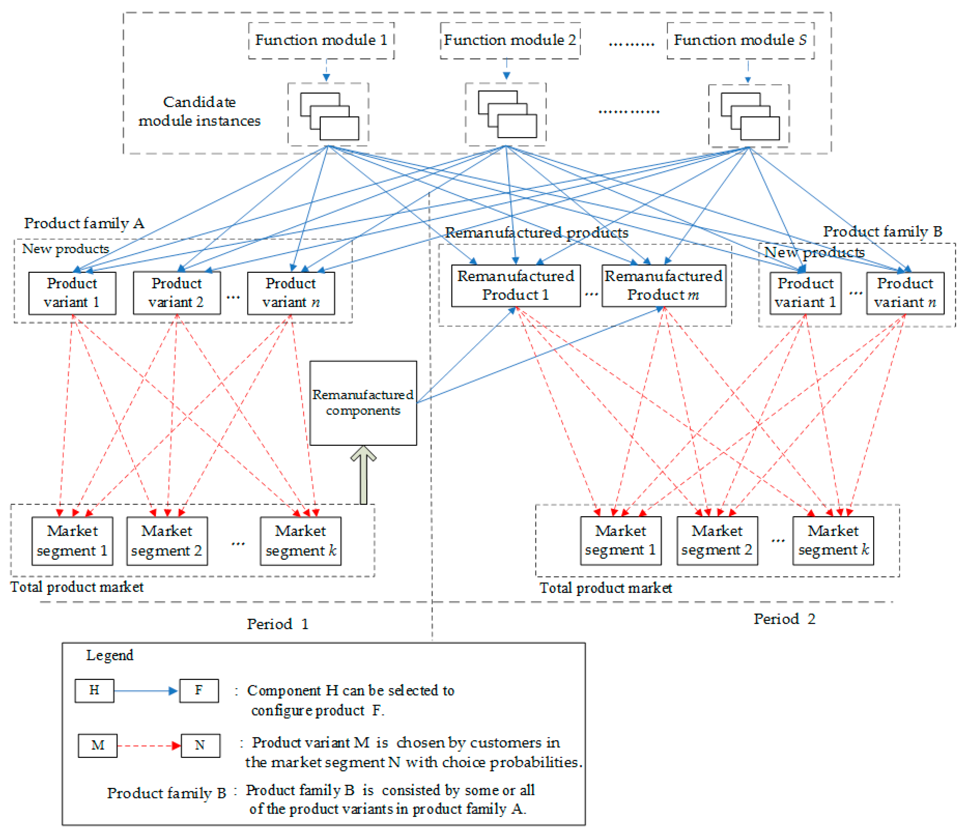
3. Problem Description

The optimization problem is described as follows: it is assumed that a product has been developed into a modular structure. That is, a product is considered to consist of a set of functional modules. Each functional module has several candidate module instances (components), and different module instances of a module have similar functionality, but different levels of performance. To meet diversified market demands, the firm wants to develop a product family. The product family contains multiple product variants, and the firm needs to choose the module instance (component) for each functional module of all product variants. Considering market demand and environmental benefits, the firm is also ready to sell remanufactured product in the later period, and remanufactured products are planned in product family design stage, simultaneously.

As shown in Figure 1, two periods are considered in this research. In period 1, a firm only offers new products to the market. In period 2, the firm introduces remanufactured products into the market. In other words, in period 2, the firm began offering both new products and remanufactured products. Some components of remanufactured products are from used products sold to the market in period 1. The configuration of remanufactured products and product variants included in the product family are not necessarily the same. Moreover, the product variants launched in period 1 are not necessary to be launched in period 2.

The goal of the proposed optimization problem is to concurrently determine product family design and remanufactured products planning with the objectives of maximizing profit and minimizing GHG emission. Especially, the decision variables in the optimization model are as follows:

• Number of product variants and remanufactured products;
• Module instance (component) configuration of each product variant and each remanufactured product;
• Selling prices of each product variant and each remanufactured product in periods 1 and 2; and
• Selection of remanufacturing technology (remanufacturing parameters) for remanufacturing of used components.

In order to facilitate subsequent modeling, the binary decision variables are pre-defined as follows:

$$x_r=\{\begin{array}{l}1\mathrm{if}\mathrm{the}r\mathrm{th}\mathrm{product}\mathrm{variant}\mathrm{is}\mathrm{produced}\\ 0\mathrm{otherwise}\end{array}$$

(1)

$$x_h^{re}=\{\begin{array}{l}1\mathrm{if}\mathrm{the}h\mathrm{th}\mathrm{remanufactured}\mathrm{product}\mathrm{is}\mathrm{produced}\\ 0\mathrm{otherwise}\end{array}$$

(2)

$$y_{ij}^r=\{\begin{array}{l}1\mathrm{if}\mathrm{the}j\mathrm{th}\mathrm{instance}\mathrm{of}i\mathrm{th}\mathrm{module}({\mathrm{M}}_{i,j})\mathrm{is}\mathrm{selected}\mathrm{for}r\mathrm{th}\mathrm{product}\mathrm{variant}\\ 0\mathrm{otherwise}\end{array}$$

(3)

$$y_{ij}^h=\{\begin{array}{l}1\mathrm{if}\mathrm{the}j\mathrm{th}\mathrm{instance}\mathrm{of}i\mathrm{th}\mathrm{module}({\mathrm{M}}_{i,j})\mathrm{is}\mathrm{selected}\mathrm{for}h\mathrm{th}\mathrm{remanufactured}\mathrm{product}\\ 0\mathrm{otherwise}\end{array}$$

(4)

$$z_{ij}^h=\{\begin{array}{l}1\mathrm{if}\mathrm{the}j\mathrm{th}\mathrm{instance}\mathrm{of}i\mathrm{th}\mathrm{module}{(\mathrm{M}}_{i,j})\mathrm{is}\mathrm{remanufactured}\mathrm{for}h\mathrm{th}\mathrm{remanufactured}\mathrm{product}\\ 0\mathrm{otherwise}\end{array}$$

(5)

4. Development of an Optimization Model

4.1. Customer Preference Modeling with Utility Function

In this article, it is assume that a product market has been divided into several market segments. The Fuzzy C-Means (FCM) clustering algorithm can be used to identify the market segment [35]. The purchasing preferences of consumers in the same segment are considered to be similar.

In the product design evaluation, utility functions are widely used to measure customer preferences, and it is adopted in this research. According to the part-worth model [36], the utility of the rth product variant in the qth segment ($u_{pro}^{r(q)}$) can be expressed as below:

$$u_{pro}^{r(q)}={\displaystyle \sum _{i=1}^I{\displaystyle \sum _{j=1}^J{y}_{{}_{ij}}^{(r)}}}{\mu }_{ij}^{(q)}+{\eta }_r(q=1,\dots ,Q)$$

(6)

where ${\mu }_{ij}^{(q)}$ is the utility of M_i,j in the qth segment, and it is measured by money.

Considering the sales price of products, the surplus utility of rth product variant in the qth segment (${\lambda }^{r(q)}$) is expressed as below:

$${\lambda }^{r(q)}=u_{pro}^{r(q)}-p_r$$

(7)

where $p_r$ is the sale price of rth product variant.

Similar to a new product, the surplus utility of the hth remanufactured product in the qth segment (${\lambda }_{re}^{h(q)}$) can be calculated as follows:

$${\lambda }_{re}^{h(q)}=u_{re}^{h(q)}-p_{re}^h$$

(8)

where $u_{re}^{h(q)}$ is the utility of the hth remanufactured product in the qth segment, $p_{re}^h$ represents the sale price of hth remanufactured product.

4.2. Product Demand Model

Generally, the purchase decision of a customer on a product is mainly affected by the surplus utility of the product and other competing products. In many studies, the probabilistic choice rule is applied to express the customer’s purchase behavior. In the probabilistic choice rule, it is assumed that the utility is a random variable and the customers choosing products follow random utility maximization criterion. Among all the probabilistic choice rules, the multinomial logic choice (MNL) rule is widely applied, and it is also adopted by this research.

In period 1, a company only offers new products to market, and the choice probability of a customer towards rth product variant in the qth segment is formulated as below:

$$P_{r-per1}^{(q)}=\frac{e^{\mu {\lambda }^{r(q)}}}{{\displaystyle \sum _{r=1}^R{e}^{\mu {\lambda }_{}^{r(q)}}}+{\displaystyle \sum _{r=1}^{N^e}{e}^{\mu {\lambda }_e^{r(q)}}}+{\displaystyle \sum _{r=1}^{N^c}{e}^{\mu {\lambda }_c^{r(q)}}}}$$

(9)

where $P_{r-per1}^{(q)}$ represents the choice probability of the rth product variant chosen in the qth market segment in period 1. R indicates the number of product variant launched to market in period 1. $N^e$ and $N^c$ are the number of competing products and the number of similar products that have been launched to markets by this company, respectively. Finally, ${\lambda }_e^{r(q)}$ and ${\lambda }_c^{r(q)}$ are the surplus utility of competing products and similar products, respectively.

In period 1, the demand of rth product variant in the qth market segment ($Q_{r-per1}^{(q)}$) is estimated as below:

$$Q_{r-per1}^{(q)}=n_{q-1}{P}_{r-per1}^{(q)}$$

(10)

where n_q-1 is the total product demand of the qth market segment in period 1.

In period 2, the company sells not only new products but also remanufactured products. The choice probability of the rth product variant chosen in the qth market segment is formulated as below:

$$P_{r-per2}^{(q)}=\frac{e^{\mu {\lambda }^{r(q)}}}{{\displaystyle \sum _{r=1}^v{e}^{\mu {\lambda }_{}^{r(q)}}}+{\displaystyle \sum _{r=1}^{N^e}{e}^{\mu {\lambda }_e^{r(q)}}}+{\displaystyle \sum _{r=1}^{N^c}{e}^{\mu {\lambda }_c^{r(q)}}}+{\displaystyle \sum _{r=1}^H{e}^{\mu {\lambda }_{re}^{h(q)}}}}$$

(11)

where v represents the number of product variants launched to markets in period 2, H is the number of remanufactured products launched to markets in period 2.

In period 2, the demand of the rth product variant in the qth market segment ($Q_{r-per2}^{(q)}$) is estimated as below:

$$Q_{r-per2}^{(q)}=n_{q-2}{P}_{r-per2}^{(q)}$$

(12)

where n_q-2 is the total product demand of the qth market segment in period 2.

The choice probability towards the hth remanufactured product in the qth market segment is formulated as below:

$$P_{h-per2}^{(q)}=\frac{e^{\mu {\lambda }_{re}^{h(q)}}}{{\displaystyle \sum _{r=1}^v{e}^{\mu {\lambda }_{}^{r(q)}}}+{\displaystyle \sum _{r=1}^{N^e}{e}^{\mu {\lambda }_e^{r(q)}}}+{\displaystyle \sum _{r=1}^{N^c}{e}^{\mu {\lambda }_c^{r(q)}}}+{\displaystyle \sum _{h=1}^H{e}^{\mu {\lambda }_{re}^{h(q)}}}}$$

(13)

In period 2, the demand of the hth remanufactured product in the qth market segment ($Q_{h-per2}^{(q)}$) is calculated as follows:

$$Q_{h-per2}^{(q)}=n_{q-2}{P}_{h-per2}^{(q)}$$

(14)

The total expected revenue of the company (T_rev) is from the sale of new products and remanufactured products, it is formulated as below:

$$T_{rev}={\displaystyle \sum _{q=1}^Q{\displaystyle \sum _{r=1}^R{Q}_{r-per1}^{(q)}{p}_{r-per1}}}+{\displaystyle \sum _{q=1}^Q{\displaystyle \sum _{r=1}^R{Q}_{r-per2}^{(q)}{p}_{r-per2}}}+{\displaystyle \sum _{q=1}^Q{\displaystyle \sum _{h=1}^H{Q}_{h-per2}^{(q)}{p}_{h-per2}}}$$

(15)

where $p_{r-per1}$ is the sale price for the rth product variant in period 1, $p_{r-per2}$ represents the sale price for the rth product variant in period 2, $p_{h-per2}$ is the sale price of the hth remanufactured product.

4.3. Cost Models

The total cost (C) includes two parts: the production cost of new products (C_new) and the production cost of remanufactured products (C_re). C is expressed as below:

$$C=C_{new}^{}+C_{re}^{}$$

(16)

(1) Production cost of new products ($C_{new}$)

$C_{new}$ consists of two parts: intra-firm production cost and purchasing cost, and it is expressed as below:

$$C_{new}=C_{}^{\mathrm{intra}}+C_{}^{pur}$$

(17)

$C^{\mathrm{intra}}$ is the cost in the production processes of products inside the firm. It can be further divided into two parts, fixed cost part ($C^{\mathrm{intra}\left(\mathrm{fix}\right)}$) and the variable cost part ($C^{\mathrm{intra}\left(\mathrm{var}\right)}$). $C^{\mathrm{intra}\left(\mathrm{fix}\right)}$ mainly includes the product development cost, managed cost, etc. $C^{\mathrm{intra}\left(\mathrm{var}\right)}$ mainly refers to the assembly cost, packaging cost, and so on.

$C^{\mathrm{intra}\left(\mathrm{fix}\right)}$ has a direct relationship with the number of developed product variant (N_pr), and it is expressed as below:

$$C^{\mathrm{intra}\left(\mathrm{fix}\right)}=\{\begin{array}{l}{Y}_1\mathrm{if}{N}_{pr}=1\\ Y_2\mathrm{if}{N}_{pr}=2\\ ⋮\\ Y_v\mathrm{if}{N}_{pr}=V\end{array}$$

(18)

where Y_v is the fixed cost part of the intra-firm production cost for a product family which has V product variants.

$C^{\mathrm{intra}\left(\mathrm{var}\right)}$ is further divided into two parts, and it is as follows:

$$C^{\mathrm{intra}\left(\mathrm{var}\right)}=C_{per1}^{\mathrm{intra}\left(\mathrm{var}\right)}+C_{per2}^{\mathrm{intra}\left(\mathrm{var}\right)}$$

(19)

where $C_{per1}^{\mathrm{intra}\left(\mathrm{var}\right)}$ and $C_{per2}^{\mathrm{intra}\left(\mathrm{var}\right)}$ are the variable cost of manufacturing new product in period 1 and in period 2, respectively.

$C_{per1}^{\mathrm{intra}\left(\mathrm{var}\right)}$ is expressed as below:

$$C_{per1}^{\mathrm{intra}\left(\mathrm{var}\right)}={\displaystyle \sum _{q=1}^Q{\displaystyle \sum _{r=1}^R{\displaystyle \sum _{i=1}^I{\displaystyle \sum _{j=1}^J{Q}_{r-per1}^{(q)}{c}_{ij}^{\mathrm{intra}\left(\mathrm{var}\right)}{y}_{ij}^{(r)}}}}}$$

(20)

where $c_{ij}^{\mathrm{intra}\left(\mathrm{var}\right)}$ is the unit variable production cost for M_i,j.

Similarly, $C_{per2}^{\mathrm{intra}\left(\mathrm{var}\right)}$ is expressed as:

$$C_{per2}^{\mathrm{intra}\left(\mathrm{var}\right)}={\displaystyle \sum _{q=1}^Q{\displaystyle \sum _{r=1}^R{\displaystyle \sum _{i=1}^I{\displaystyle \sum _{j=1}^J{Q}_{r-per2}^{(q)}{c}_{ij}^{\mathrm{intra}\left(\mathrm{var}\right)}{y}_{ij}^{(r)}}}}}$$

(21)

By combining Equations (18), (19), (20), and (21), $C^{\mathrm{intra}}$ is reformulated as below:

$$C^{\mathrm{intra}}=Y_v+{\displaystyle \sum _{q=1}^Q{\displaystyle \sum _{r=1}^R{\displaystyle \sum _{i=1}^I{\displaystyle \sum _{j=1}^J{Q}_{r-per1}^{(q)}{c}_{ij}^{\mathrm{intra}\left(\mathrm{var}\right)}{y}_{ij}^{(r)}+}}}}{\displaystyle \sum _{q=1}^Q{\displaystyle \sum _{r=1}^R{\displaystyle \sum _{i=1}^I{\displaystyle \sum _{j=1}^J{Q}_{r-per2}^{(q)}{c}_{ij}^{\mathrm{intra}\left(\mathrm{var}\right)}{y}_{ij}^{(r)}}}}}$$

(22)

The purchasing cost for selected module instances ($C^{\mathrm{pur}\left(\mathrm{var}\right)}$) is expressed as follows:

$$C^{\mathrm{pur}\left(\mathrm{var}\right)}={\displaystyle \sum _{i=1}^I{\displaystyle \sum _{j=1}^J{\displaystyle \sum _{q=1}^Q{\displaystyle \sum _{r=1}^R(Q_{r-per1}^{(q)}+Q_{r-per2}^{(q)})y_{ij}^{(r)}{x}_r{p}_{ij}}}}}$$

(23)

where $p_{ij}$ indicates the purchase price for M_i,j.

(2) Production cost of remanufactured products ($C_{re}$)

The production cost for remanufactured products mainly includes remanufacturing cost of used components ($C_{re}^{re-c}$), the purchase cost of new components ($C_{re}^{n-c}$) and variable production cost ($C_{re}^{\mathrm{var}}$), and it is expressed as follows:

$$C_{re}=C_{re}^{re-c}+C_{re}^{n-c}+C_{re}^{\mathrm{var}}$$

(24)

Remanufacturing cost indicates the cost associated with collecting used products ($C_{reco}$) and the remanufacturing cost of used components ($C_{remanu}$), and it is expressed as follows:

$$C_{re}^{re-c}=C_{reco}+C_{remanu}$$

(25)

The cost of collecting used products is related to the number of collecting. Different from a single product, there are multiple different product variants in a product family. Due to the fact that different product variants include different numbers of components that can be used to configure remanufactured products, the cost of collecting used products is different with the recovery different product variants. This research constructs an optimization model to determine the recycling amount of each product variant for the minimum recycling cost of used products. The optimization model is expressed as follows:

$$Min{C}_{reco}={\displaystyle \sum _{r=1}^R{Q}_{re-r}{c}_{re-un}^r}$$

(26)

$$s.t:{\displaystyle \sum _{h=1}^H{\displaystyle \sum _{q=1}^Q{Q}_{h-per2}^{(q)}}}{z}_{ij}^h{x}_h^{re}\ge {\displaystyle \sum _{r=1}^R{Q}_{re-r}{y}_{ij}^r(i=1,2,\dots ,I;j=1,2,\dots ,J)}$$

(27)

$$0\le Q_{re-r}\le {\displaystyle \sum _{q=1}^Q{Q}_{r-per1}^{(q)}}(r=1,2,\dots ,R)$$

(28)

where $Q_{re-r}$ represents the recycling number of rth product variant, $c_{re-un}^r$ is the unit cost of recycling rth product variant. Constraint (27) ensures that the number of each required remanufactured components can be satisfied. Constraint (28) ensures that recycling number of the rth product variant less than the number of sales in period 1.

The remanufacturing cost of the used components is related to the remanufacturing technology. By adopting different remanufacturing technologies, the used component can achieve different reliability values of component. For the sake of clarity, here, the selected remanufacturing technology for a used component is indicated by the achieved reliability of the component after remanufacturing. With adopting different remanufacturing technologies, the remanufacturing cost of a used component is different. The remanufacturing cost can be expressed as below:

$$C_{remanu}={\displaystyle \sum _{q=1}^Q{\displaystyle \sum _{h=1}^H{\displaystyle \sum _{i=1}^I{\displaystyle \sum _{j=1}^J{Q}_{h-per2}^{(q)}}}}}{x}_h^{re}{Z}_{ij}^h{V}_{ij}$$

(29)

$$V_{ij}=\{\begin{array}{l}{V}_1\mathrm{if}{R}_{ij}^{re}=R_1\\ V_2\mathrm{if}{R}_{ij}^{re}=R_2\\ ⋮\\ V_v\mathrm{if}{R}_{ij}^{re}=R_{\nu }\end{array}$$

(30)

where V_ij represents the remanufacturing cost per unit component M_i,j (the jth instance of the ith module), $R_{ij}^{re}$ is the value of reliability for component M_i,j after remanufacturing, R_V indicates that the value of reliability can be achieved by M_i,j if the vth remanufacturing technology is adopted.

In a remanufactured product, not all the components are used components. Some new components need to be purchased. The purchase cost of new components for remanufactured products is expressed as follows:

$$C_{re}^{\mathrm{n}-\mathrm{c}}={\displaystyle \sum _{Q=1}^Q{\displaystyle \sum _{h=1}^H{\displaystyle \sum _{i=1}^I{\displaystyle \sum _{j=1}^J{Q}_{h-\mathrm{per}2}^{(q)}{x}_h^{re}{y}_{ij}^h{p}_{ij}^{}}}}}$$

(31)

The variable production cost (e.g., assembly cost) for remanufactured products is as follows:

$$C_{re}^{\mathrm{var}}={\displaystyle \sum _{q=1}^Q{\displaystyle \sum _{h=1}^H{\displaystyle \sum _{i=1}^I{\displaystyle \sum _{j=1}^J{Q}_{h-pre2}^{(q)}{x}_h^{re}{y}_{ij}^h{z}_{ij}^h{c}_{ij}^{\mathrm{intra}\left(\mathrm{var}\right)}}}}}$$

(32)

4.4. GHG Emission Models

The total GHG emission, from new and remanufactured products, is expressed as follows:

$$E=E_{new}+E_{rema}$$

(33)

where $E_{new}$ is the GHG emission from new products, $E_{rema}$ represents the GHG emission from remanufactured products.

$E_{new}$ contains the GHG emission from component ($E_{new}^{com}$) and product assemble ($E_{new}^{ass}$).

$$E_{new}=E_{new}^{com}+E_{new}^{ass}$$

(34)

$$E_{new}^{com}={\displaystyle \sum _{i=1}^I{\displaystyle \sum _{j=1}^J{\displaystyle \sum _{q=1}^Q{\displaystyle \sum _{r=1}^R(Q_{r-per1}^{(q)}+Q_{r-per2}^{(q)})y_{ij}^r{e}_{ij}}}}}$$

(35)

$$E_{new}^{\mathrm{var}}={\displaystyle \sum _{i=1}^I{\displaystyle \sum _{j=1}^J{\displaystyle \sum _{q=1}^Q{\displaystyle \sum _{r=1}^R(Q_{r-per1}^{(q)}+Q_{r-per2}^{(q)})y_{ij}^r{e}_{ij}^{\mathrm{var}}}}}}$$

(36)

where $e_{ij}$ is the GHG emission of M_i,j, $e_{ij}^{\mathrm{var}}$ indicates the GHG emission of module instance M_i,j in the assembly stage.

$E_{rema}$ contains the GHG emission from collecting used products ($E_{rema}^{col}$), disposing used products ($E_{rema}^{dis}$), remanufacturing of used components ($E_{rema}^{re-com}$), new components ($E_{rema}^{new}$) and the assembly of remanufactured products ($E_{rema}^{ass}$), and it is expressed as follows:

$$E_{rema}=E_{rema}^{col}+E_{rema}^{dis}+E_{rema}^{re-com}+E_{rema}^{new}+E_{rema}^{ass}$$

(37)

$E_{rema}^{col}$ is related to the number of used products collecting and the GHG emission per unit of used product collecting, and it is expressed as follows:

$$E_{rema}^{col}={\displaystyle \sum _{r=1}^R{Q}_{re-r}}{e}_{col}$$

(38)

where $e_{col}$ is the GHG emission from per unit of used product collecting.

$E_{rema}^{dis}$ is associated with the number of used product disposing and the GHG emission from per unit of used product disposing, and it is expressed as follows:

$$E_{rema}^{dis}={\displaystyle \sum _{r=1}^R{Q}_{re-r}}{e}_{dis}$$

(39)

$$e_{dis}={\displaystyle \sum _{w=1}^W{\displaystyle \sum _{f=1}^F{E}_w^f}}{e}^f$$

(40)

where $e_{dis}$ is the GHG emission from per unit of used product disposing. $E_w^f$ is the amount of fth energy consumption in wth treatment processes, W is the number of treatment processes, F is the number of energy consumption in treatment processes, $e^f$ indicates carbon emission factor of fth energy.

Similar to remanufacturing cost, the GHG emission of a used component produced in remanufacturing process is also different with adopting different remanufacturing technologies. The $E_{rema}^{re-com}$ can be expressed as below:

$$E_{rema}^{re-com}={\displaystyle \sum _{q=1}^Q{\displaystyle \sum _{h=1}^H{\displaystyle \sum _{i=1}^I{\displaystyle \sum _{j=1}^J{Q}_{h-per2}^{(q)}}}}}{x}_h^{re}{z}_{ij}^h{e}_{ij}^{re}$$

(41)

$$e_{ij}^{re}=\{\begin{array}{l}{e}_{ij}^{re-1}\mathrm{if}{R}_{ij}^{re}=R_1\\ e_{ij}^{re-2}\mathrm{if}{R}_{ij}^{re}=R_2\\ ⋮\\ e_{ij}^{re-v}\mathrm{if}{R}_{ij}^{re}=R_{\nu }\end{array}$$

(42)

$$e_{ij}^{re-v}={\displaystyle \sum _{k=1}^K{\displaystyle \sum _{p=1}^P{E}_k^{p(v)}{e}^p}}(v=1,2,\dots ,V)$$

(43)

where $e_{ij}^{re}$ is the remanufacturing GHG emission per unit component M_i,j (jth instance of ith module), $e_{ij}^{re-v}$ represents the remanufacturing GHG emission per unit component M_i,j when the vth remanufacturing technology is adopted, $E_k^{p(v)}$ is the amount of kth energy consumption using the vth remanufacturing technology in the pth remanufacturing production process, $e^p$ represents carbon emission factor of pth energy.

$E_{rema}^{new}$ represents the GHG emission from new components for remanufactured products, and it can be expressed as below:

$$E_{rema}^{\mathrm{new}}={\displaystyle \sum _{q=1}^Q{\displaystyle \sum _{h=1}^H{\displaystyle \sum _{i=1}^I{\displaystyle \sum _{j=1}^J{Q}_{h-\mathrm{per}2}^{(q)}{y}_{ij}^h{e}_{ij}^{}}}}}$$

(44)

$E_{rema}^{ass}$ is the GHG emission of remanufactured product from the assembly stage, and it calculated as follows:

$$E_{re}^{ass}={\displaystyle \sum _{q=1}^Q{\displaystyle \sum _{h=1}^H{\displaystyle \sum _{i=1}^I{\displaystyle \sum _{j=1}^J{Q}_{h-per2}^{(q)}{y}_{ij}^h{z}_{ij}^h{e}_{ij}^{\mathrm{ass}}}}}}$$

(45)

4.5. Constraints

4.5.1. Selection Constraint of Module Instances.

Each functional module of each product variant can only choose one module instance, and the constraint is expressed as follows:

$${\displaystyle \sum _{j=1}^J{y}_{ij}^r}=1,(r=1,2,\dots ,R;i=1,2,\dots ,I)$$

(46)

4.5.2. Selection Constraint of Remanufactured Components for Remanufactured Products

If a product does not contain a remanufactured component, the product is not a remanufactured product. That is, a remanufactured product needs to choose at least one remanufactured component. This selection constraint can be expressed as follows:

$${\displaystyle \sum _{i=1}^I{\displaystyle \sum _{j=1}^J{Z}_{ij}^h}}\ge 1,(h=1,2,\dots ,H)$$

(47)

4.5.3. Product Reliability Constraint

Reliability is related to product’s safety and operating performance of product under specified conditions. No matter new products or remanufactured products, the reliability of products needs to satisfy a specific level. The product reliability constraint for a new product can be expressed as follows:

$${\displaystyle \prod _{i=1}^I{\displaystyle \prod _{j=1}^J{R}_{ij}{y}_{ij}^r\ge R_n,(r=1,2,\dots ,R)}}$$

(48)

where $R_n$ indicates the reliability that a new product needs to be satisfied, $R_{ij}$ is the reliability of module instance M_i,j, and it is expressed as follows:

$$R_{ij}=\{\begin{array}{ll}1& if{y}_{ij}^r=0\\ R_{ij}& otherwise\end{array}(r=1,2,\dots ,R;i=1,2,\dots ,I;j=1,2,\dots ,J)$$

(49)

The product reliability constraint for a remanufactured product is formulated as follows:

$${\displaystyle \prod _{i=1}^I{\displaystyle \prod _{j=1}^J{R}_{ij}{y}_{ij}^h{R}_{ij}^{re}{z}_{ij}^h\ge R_r}}(h=1,2,\dots ,H)$$

(50)

$$R_{ij}=\{\begin{array}{ll}1& if{y}_{ij}^h=0\\ R_{ij}& otherwise\end{array}(h=1,2,\dots ,H;i=1,2,\dots ,I;j=1,2,\dots ,J)$$

(51)

$$R_{ij}^{re}=\{\begin{array}{ll}1& if{z}_{ij}^r=0\\ R_{ij}^{re}& otherwise\end{array}(h=1,2,\dots ,H;i=1,2,\dots ,I;j=1,2,\dots ,J)$$

(52)

where $R_{ij}^{re}$ is the reliability of module instance M_i,j after remanufacturing, $R_r$ represents the reliability that a remanufactured product need to be satisfied.

4.6. Formulation of the Optimization Model

The proposed optimization problem is able to formulate as a constrained programming problem. Based on the above analysis, the optimization model can be established as below:

$$\begin{array}{l}\mathrm{Objective}1:\mathrm{Max}\Delta =T_{rev}-C\\ \mathrm{Objective}2:\mathrm{Min}E\\ s.t.Eqs.(46-52)\\ x_r^n,x_h^{re},y_{ij}^r,y_{ij}^h,z_{ij}^h\in \{0,1\},p_{r-per1}>0,p_{r-per2}>0\mathrm{and}{p}_{h-per2}>0\end{array}$$

(53)

Notations:

$\Delta$	Total profit of a company
$T_{rev}$	Total expected revenue of a company
C	Total cost of production
E	Total GHG emission of production
$x_r^n$	Binary decision variable such that $x_r^n=1$ if the rth product variant is produced, and $x_r^n=0$ otherwise
$x_h^{re}$	Binary decision variable such that $x_h^{re}=1$ if the hth remanufactured product is produced, and $x_h^{re}=0$ otherwise
$y_{ij}^r$	Binary decision variable such that $y_{ij}^r=1$ if the jth instance of ith module is selected for rth product variant, and $y_{ij}^r=0$ otherwise
$y_{ij}^h$	Binary decision variable such that $y_{ij}^h=1$ if the jth instance of ith module is selected for hth remanufactured product, and $y_{ij}^h=0$ otherwise
$z_{ij}^h$	Binary decision variable such that $z_{ij}^h=1$ if the jth instance of ith module is remanufactured for hth remanufactured product, and $z_{ij}^h=0$ otherwise
$p_{r-per1}$	Sale price of rth product variant in period 1
$p_{r-per2}$	Sale price of rth product variant in period 2
$p_{h-per2}$	Sale price of hth remanufactured product

5. Solution Methodology

The proposed optimization model is hard to be solved by classical mathematical programming methods due to non-linearity of the optimization problem. In dealing with such problems, the heuristic algorithm is more effective than the traditional algorithms. Many heuristic algorithms, such as genetic algorithm, simulated annealing and particle swarm algorithm, have been proposed to solve multi-objective optimization problems. Owing to its simple computation and robust search ability (Mukhopadhyay et al. [37]; Wang et al. [38]), genetic algorithm has been successfully used to solve various multi-objective problems, and it is adopted in this paper. The description of the proposed GA is presented in the following sub-section.

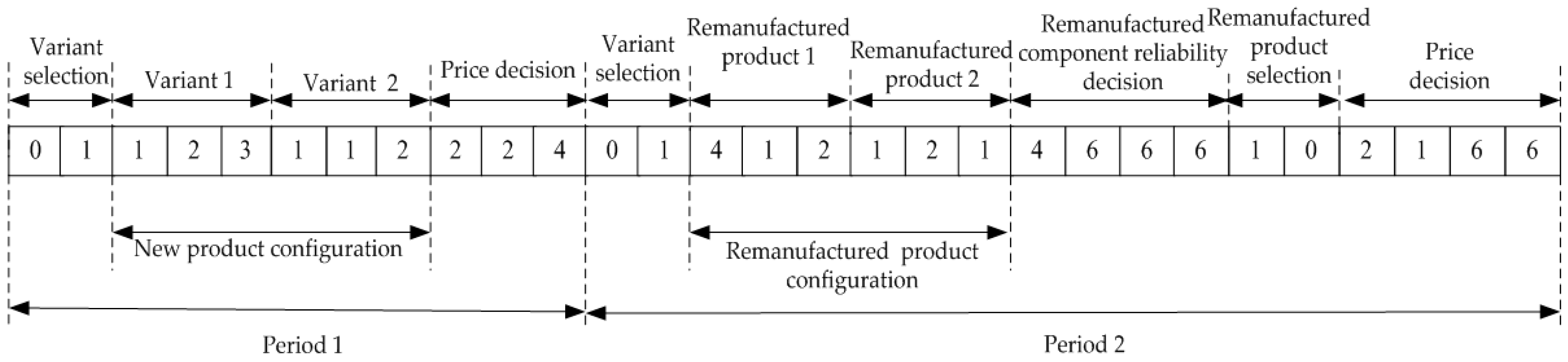
5.1. Chromosome Representation

The integer-coding approach is used in this article. A chromosome consists of two sections: a period 1 section and a period 2 section. Each section is further divided into several sub-sections. An example of a chromosome is shown in Figure 2. In the period 1 section, there are P genes in sub-section of variant selection, and the value ‘1’ in the pth gene indicates that the pth product variant is chosen for the product family, and ‘0’ otherwise. The sub-section of product variant configuration indicates the instance configuration of each product variant. For example, the value ‘1’ in the first gene of product variant configuration section represents that M_1,1 is chosen for configuring the M₁ of variant 1. In the price decision sub-section, the value in the gene points out the choice of price for the corresponding product variant. In the period 2 section, there are also several sub-sections. For example, in variant selection sub-section, the gene value indicates which product variants are launched to the market in period 2. The sub-section of remanufactured product configuration indicates the module instance configuration of each remanufactured product. In the reliability decision sub-section of remanufactured component, the gene value indicates which remanufacturing technology/process (parameters) is applied for the corresponding remanufactured component. The selection sub-section of remanufactured product represents which remanufactured products are launched to the market. The sub-section of price decision indicates which price is selected for the corresponding product in period 2 (including product variants and remanufactured products).

5.2. Fitness Function

In previous studies, many methods have been proposed for solving multi-objective optimization problems. A widely applied, simple, and useful way is the weighted additive utility function, and it is adopted in this research. Two positive weights u₁ and u₂ (u₁ + u₂ = 1) is assigned to the goals. Here, the weight u₁ is used to measure profit (f₁), and the weight u₂ measures GHG emission (f₂). The size of each weight indicates the importance of the associate objective. Owing to the fact that the scale of the two objectives (profit and GHG emission) is different, the two objectives need to be normalized separately. The weighted additive utility function with normalized objectives is formulated as follows:

$$F^{\prime }(k)=u_1{f}_1\prime (k)+u_2{f}_2\prime (k)$$

(54)

where $f_i\prime$ indicates the normalized value which can be expressed as:

$$f_i\prime (k)=\frac{f_i(k)-f_{i,\min }}{f_{i,\max }-f_{i,\min }}$$

(55)

where $f_{i,\min }$ and $f_{i,\max }$ are the minimum and maximum values for $f_i(k)$, respectively.

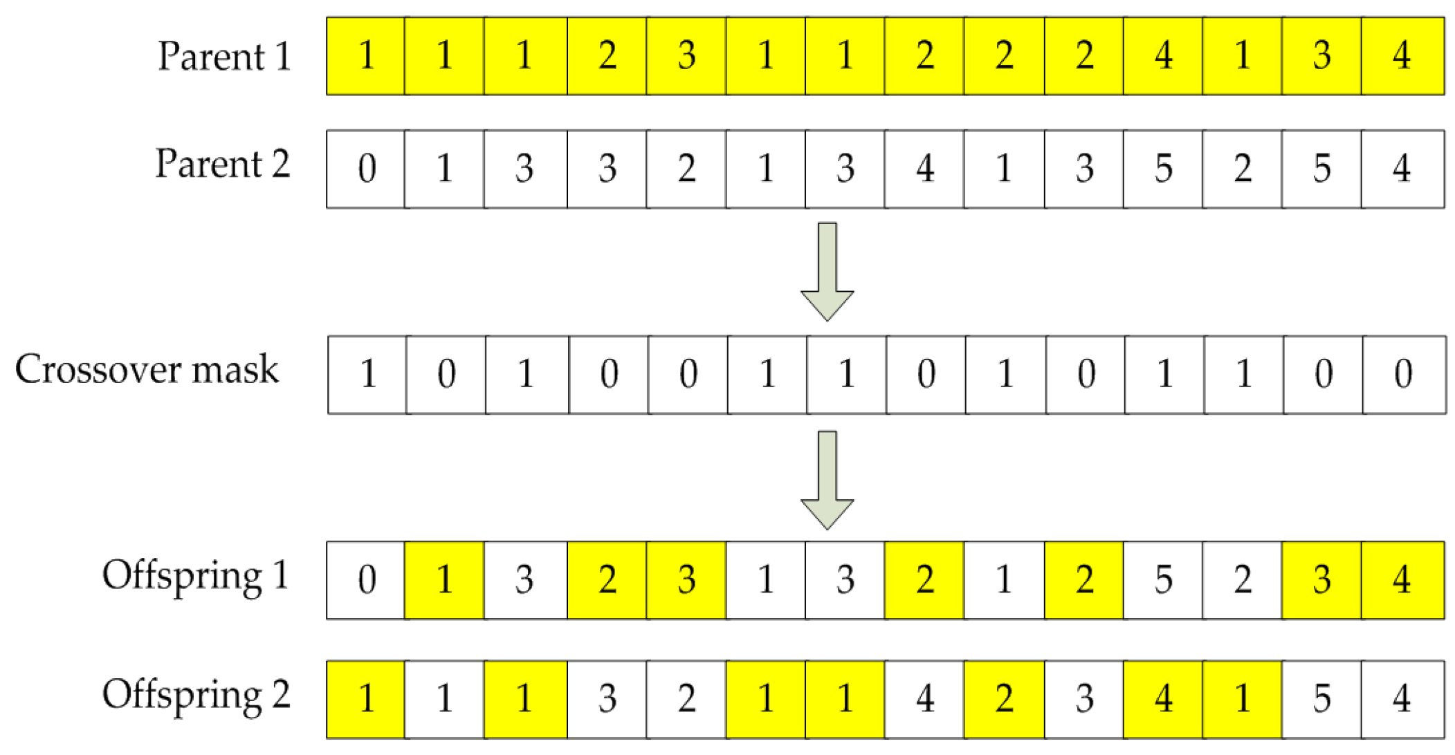
5.3. Genetic Operators

(i) Crossover. Here, the uniform crossover method is applied. There are two steps in the crossover process. Firstly, a crossover mask with the value of 0 or 1 is randomly produced. Secondly, the gen values of two parents are swapped if the corresponding crossover mask value is 1. Figure 3 provides an example for the crossover operation, the offspring is generated according to the crossover mask.

(ii) Mutation. In this research, the mutation operation of GA is performed according to the neighborhood idea. Here, the neighborhood of a gene is considered as the incremental or decremental change to the gene value. An individual mutates with a probability. The mutation randomly selects some genes and then changes the values of gene to their neighborhood.

(iii) Selection mechanism. The roulette selection operator is applied. In the roulette selection method, the individual with greater fitness has a higher probability of being selected as a parent to generate the offspring in the next generation.

5.4. Constraints Handling

There are various constraints in the optimization problem. The feasible solution of the optimization problem needs to satisfy all constraints. To eliminate infeasible solutions, the punishment function approach is used in this article, and it can be expressed as below:

$$H(x)=eval(x)+p(x)$$

(56)

$$p(x)=\{\begin{array}{l}0\mathrm{if}\mathrm{x}\mathrm{is}\mathrm{a}\mathrm{feasible}\mathrm{chromosome}\\ L\mathrm{otherwise}\end{array}$$

(57)

6. Case Study

An air conditioner manufacturer is ready to develop a family of air conditioners. The product is planned into a modular structure comprised of six modules. The six modules are as follows: frequency conversion module (M₁), control module (M₂), power module (M₃), temp-control module (M₄), radio transmitting/receiving module (M₅), and casting module (M₆). Each module includes several module instances (components), and different module instances of a module have similar functionality but different level of performance. Considering the customer needs and environmental benefits, the company prepares to sell remanufactured products in the later period.

After a market survey and analysis, the product market is divided into three market segments. The product demands in two periods for three market segments are provides in

Table 1. The surpluses utility ($) of the competitive products and market size.

-	Segment 1	Segment 2	Segment 3
Demand quantity (PCS) period 1/2	250,000/40,0000	400,000/360,000	650,000/380,000
Utility of competitor product 1	85.48	98.27	156.87
Utility of competitor product 2	120.47	110.62	107.58

. Two competitive products exist in the market, and surplus utilities of competitive products are also shown in Table 1. Related information for new components is provided in

Table 2. Related information of components.

Module	Module Instance (Component) (Price, $)	Utility in Segment 1	Utility in Segment 2	Utility in Segment 3	Variable Unit Cost ($)	Variable Unit Emission (g)	GHG Emission (g)	Reliability
M1	M1,1 (82.45)	160.65	164.40	155.20	8	3	40.9	0.988
	M1,2 (75.48)	152.31	153.29	147.45	8	5	37.2	0.983
	M1,3 (70.47)	145.52	148.85	140.10	10	3	35.4	0.985
	M1,4 (65.08)	140.56	138.30	134.90	10	3	30.3	0.985
M2	M2,1(76.58)	110.23	108.21	115.87	7	1	217	0.999
	M2,2 (70.25)	105.87	103.49	107.46	8	3	210	0.997
	M2,3 (65.08)	100.68	97.84	98.45	8	1	220	0.999
	M2,4 (57.49)	97.89	89.27	84.87	9	2	198	0.998
M3	M3,1 (39.08)	50.57	52.87	47.59	7	5	282	0.987
	M3,2 (32.14)	45.98	47.85	44.12	7	5	254	0.988
	M3,3 (28.79)	41.45	38.98	35.87	8	3	264	0.986
M4	M4,1 (240.89)	300.54	298.47	307.56	6	3	362	0.995
	M4,2 (218.87)	285.25	281.28	291.58	6	1	358	0.996
	M4,3 (200.08)	274.87	270.79	284.26	8	1	341	0.998
M5	M5,1 (15.76)	27.9	28.45	27.5	7	2	157	0.986
	M5,2 (13.14)	24.86	24.47	20.89	8	3	134	0.985
	M5,3 (11.42)	22.14	18.49	16.45	8	4	130	0.982
M6	M6,1(56.11)	97.56	89.45	97.25	6	1	450	0.998
	M6,2 (50.98)	88.47	84.87	89.82	6	2	431	0.998
	M6,3 (44.38)	80.78	77.69	74.39	6	3	425	0.997

. The related remanufacturing information of some components is given in

Table 3. Remanufacturing information of components.

Module instance	Reliability	Utilities in Segment 1/2/3	Remanufacturing Unit Cost/GHG Emission
M2,1	1st: 0.978	77.16/75.74/81.10	22.97/65.1
	2st: 0.959	66.13/64.92/69.52	15.31/43.4
M2,2	1st: 0.985	74.10/72.44/75.22	21.07/63
	2st: 0.968	63.52/62.09/64.47	14.05/42
M2,3	1st: 0.985	70.04/68.48/68.91	19.52/66
	2st: 0.968	60.40/58.70/59.07	13.01/44
M2,4	1st: 0.987	68.52/62.48/59.40	17.24/59.4
	2st: 0.959	58.73/53.56/50.92	11.49/39.6
M3,1	1st: 0.978	35.39/37/33.31	11.72/84.6
	2st: 0.959	30.34/31.72/28.55	7.81/56.4
M3,2	1st: 0.968	32.18/33.49/30.88	9.64/76.2
	2st: 0.949	27.58/28.71/26.47	6.42/50.8
M3,3	1st: 0.968	29.01/27.28/25.10	8.63/79.2
	2st: 0.948	24.87/23.98/21.52	5.75/52.8
M5,1	1st: 0.969	19.53/19.91/19.25	4.72/47.1
	2st: 0.947	16.74/17.07/16.5	3.15/31.4
M5,2	1st: 0.988	17.40/17.12/14.62	3.94/40.2
	2st: 0.969	14.91/14.68/12.53	2.62/26.8
M5,3	1st: 0.988	15.49/12.94/11.51	3.42/39
	2st: 0.965	13.28/11.09/9.87	2.28/26
M6,1	1st: 0.990	68.29/62.61/68.07	16.83/135
	2st: 0.975	58.53/53.67/58.35	11.22/90
M6,2	1st: 0.990	61.92/59.40/62.87	15.29/129.3
	2st: 0.982	53.08/50.92/53.89	10.19/86.2
M6,3	1st: 0.98	56.54/54.38/52.07	13.31/127.5
	2st: 0.97	48.46/46.61/44.63	8.87/85

. By analysis of the utility and cost of a product, the possible price for a new product can be confined at [$509.4, $598.4], and the product price is discretized as a set of integer prices ranging from $510 to $600. Similarly, the price of remanufactured products is discretized from $300 to $430. As illustrated in the previous section, the GA is employed to solve the coordinated optimization design of low-carbon product family and remanufactured products for the case study. The maximum number of generations is set to 100. When the maximum number of generations is reached, the computation is terminated. The calculation is convergent in about 42 generations in the case study.

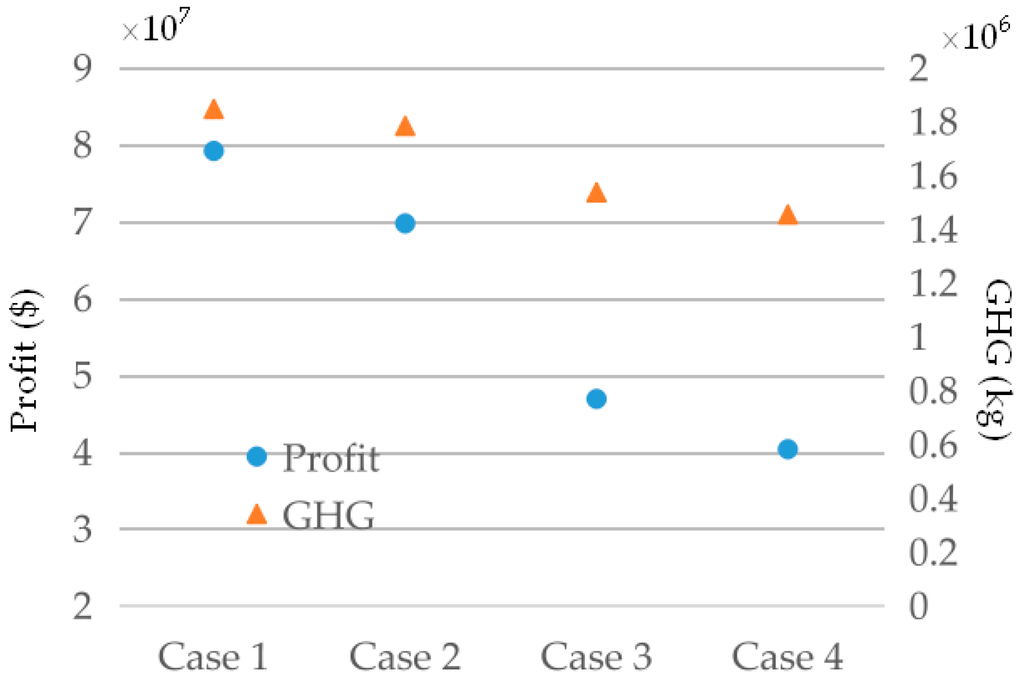
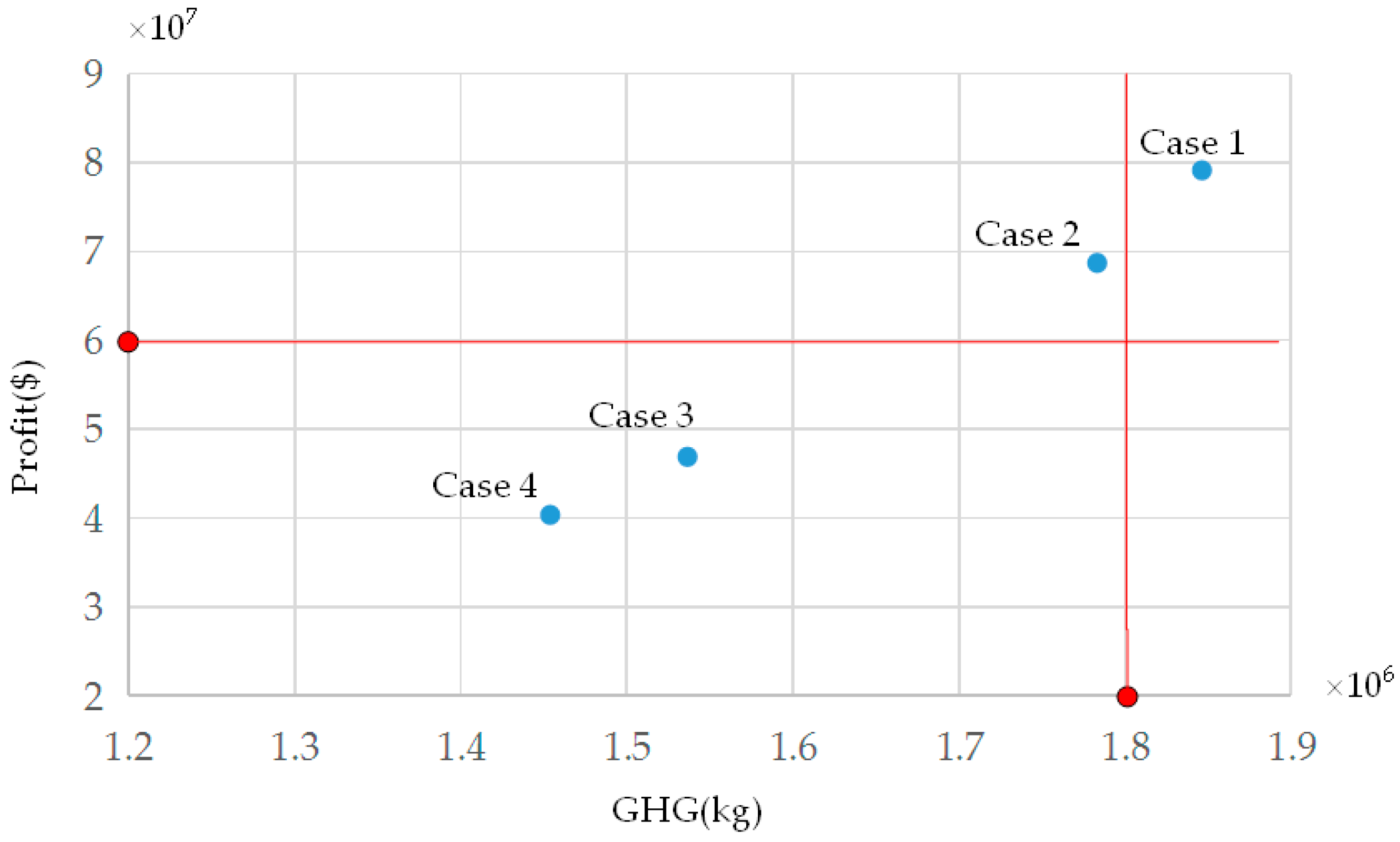
6.1. Sensitivity Analysis of GHG Emission Weight

Generally, a firm hopes to maximize profit while minimizing GHG emission in product production. Nevertheless, the two goals may be contradictory. The decision makers need to determine the size of each objective weight. When a greater weight is assigned for the objective of profit, the optimized solution can bring a higher profit. Nevertheless, it could lead to a greater GHG emission. On the contrary, when a higher weight is allocated to the objective of GHG emission, the optimized solution can bring a lower GHG emission, but the profit could be lower. For analyzing the influence of GHG emission weight on optimization results, the four cases with different weight values are discussed. The reliability threshold value of the product and objective weights for the four cases are set as follows:

R_n = R_r > 0.85. (i) Case 1: u₁ = 1, u₂ = 0; (ii) Case 2: u₁ = 0.8, u₂ = 0.2; (iii) Case 3: u₁ = 0.7, u₂ = 0.3; (iv) Case 4: u₁ = 0.5, u₂ = 0.5.

The optimal configuration schemes of product family and remanufactured products for the four cases are provided in

Table 4. The configuration of product family and remanufactured product for Cases 1–4.

		Module Instance Configuration						Launched in Period
	Product	M1	M2	M3	M4	M5	M6	1	2
Case 1	variant 1	1	1	1	3	1	2	Yes	Yes
	variant 2	2	1	2	3	2	3	Yes	Yes
	variant 3	2	4	3	1	3	2	Yes	Yes
	Remanufactured 1	3	1r−1	1r−1	2	1r−1	2	-	Yes
	Remanufactured 2	4	1r−1	3	2	1r−1	3	-	Yes
Case 2	variant 1	4	1	2	2	2	2	Yes	Yes
	variant 2	4	4	1	3	2	1	Yes	Yes
	variant 3	3	1	1	2	1	1	Yes	Yes
	Remanufactured 1	2	4	1r−1	3	1r−1	1r−1	-	Yes
	Remanufactured 2	3	1r−1	1r−1	3	1r−1	2	-	Yes
	Remanufactured 3	3	1r−1	1r−1	3	1r−1	1r−1	-	Yes
Case 3	variant 1	1	3	3	2	3	2	Yes	Yes
	variant 2	4	1	3	3	3	2	Yes	Yes
	variant 3	4	1	1	2	1	1	Yes	Yes
	Remanufactured 1	2	4	1r−1	3	1r−2	2	-	Yes
	Remanufactured 2	3	3	1r−1	3	1r−2	3	-	Yes
	Remanufactured 3	1	1r−2	1	3	1r−2	2	-	Yes
Case 4	variant 1	1	4	3	3	1	3	Yes	Yes
	variant 2	1	2	3	3	3	1	Yes	Yes
	variant 3	2	1	2	3	1	2	Yes	Yes
	Remanufactured 1	1	4	3	3	1r−2	2	-	Yes
	Remanufactured 2	3	3	3	3	1r−2	3	-	Yes
	Remanufactured 3	1	1r−1	3	2	1	3	-	Yes

^r-x denotes that a remanufactured component with the xst reliability is configured.

. It can be seen that they are not the same. The difference is reflected not only in product family design, but also reflected in remanufactured product planning. For example, two remanufactured products are planned in Case 1, and it is different from Cases 2–4 that three remanufactured products are planned. Figure 4 shows the optimization results. It is observed that there is a contradictory relationship between the two goals. All four cases present positive objective values in profit, and it means that all cases are profitable. Especially, Case 1 shows the largest profit among the four cases. Once Case 1 is adopted, the expected profit can reach $7.9161 × 10⁷. However, since Case 1 did not consider the GHG emission, the GHG emission of Case 1 had the highest value. In Case 2, the profit is mainly concerned, but the GHG emission is considered properly. The total profit of Case 2 is about 12% lower than that of Case 1 while the total GHG emission of Case 2 is about 5% lower than that of Case 1. Compared with Case 1, the number of remanufactured products is increasing, while more remanufactured components are adopted to configuration remanufactured products for reducing GHG emission. The weight set in Case 3 requires more attention to be paid to GHG emission than in Case 2. Therefore, comparing Case 3 with Case 2, the profit in Case 3 is lower than that in Case 2, but the GHG emission in Case 3 is also lower than that in Case 2. In Case 4, the reducing GHG emission and the making profit are considered equally important. Case 4 resulted in the lowest GHG emission among the four cases. Compared with Case 1, in Case 4, there is a decrease of 21% in the GHG emission, and the firm profit decreases by 49%.

These results mean that the company’s strategy and the environmental regulation are required for decision making. The Figure 5 is provided to identify the optimized design scheme. As shown in Figure 5, if the environmental regulation restricts the GHG emission to below 1.8 million kilograms, the design schemes (including product family design and remanufactured products planning) in Cases 2, 3 and 4 could be selected as shown in Table 4. In addition, when the expected profit of a company is more than 60 million dollars, the design scheme in Case 2 could satisfy both the environmental regulation and the expected profit threshold.

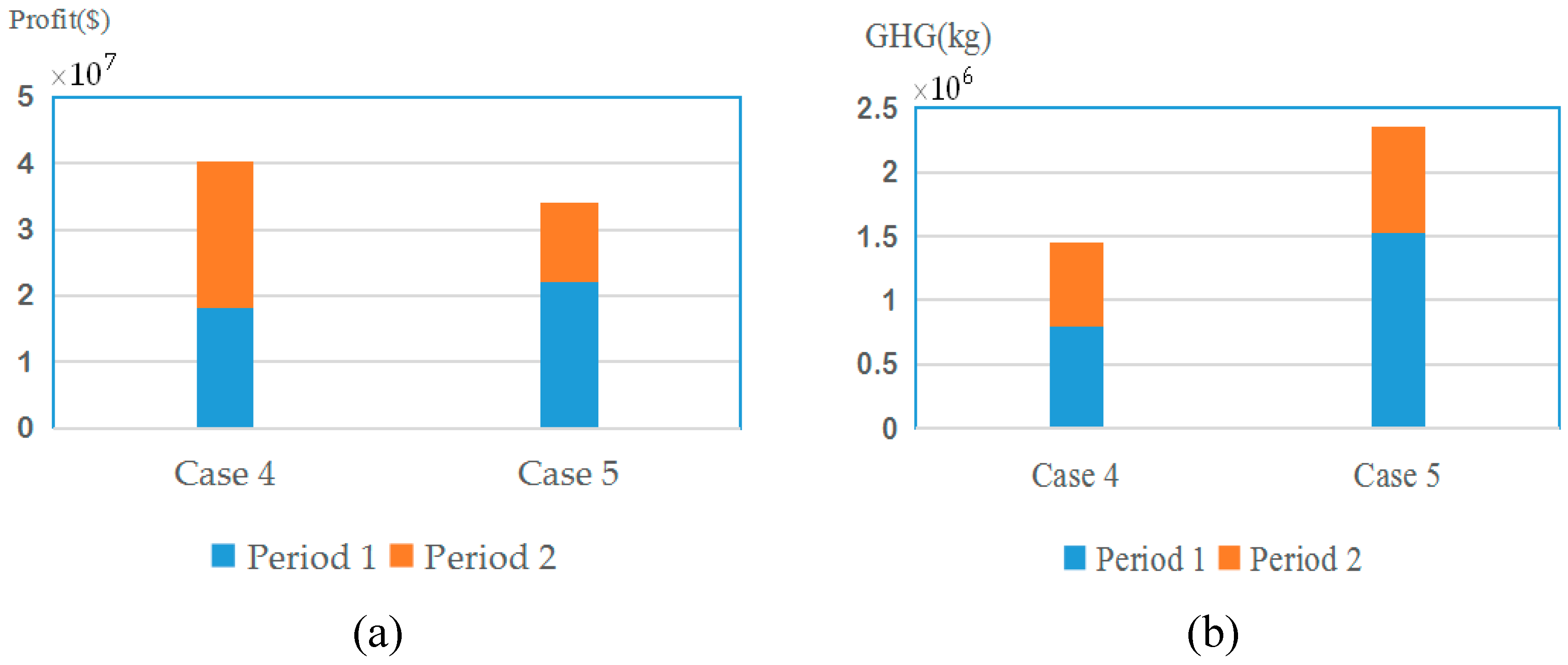
6.2. Analysis to the Effect on Low-Carbon Product Family Design with or without Considering Remanufactured Products

Case 5: u₁ = 0.5, u₂ = 0.5, without considering remanufacturing, R_n = R_r > 0.85

The integration and separation optimization of product family design and remanufactured products planning are compared to demonstrate the effectiveness of the presented approach. For comparison, Case 5 is designed. The difference between Case 4 and Case 5 is whether remanufactured products are considered in low-carbon product family design simultaneously. In Case 5, the product family design and remanufactured products planning are not simultaneously optimized, and it is decomposed into two sub-optimization problems. First, the product family is designed based on the market demand in period 1. Second, according to the design of product family and the market demand in period 2, the remanufactured products are planned, and which product variants launched to the market in period 2 are determined.

The optimized design schemes of product family and remanufactured products in Case 5 are provided in

Table 5. The configuration of product family and remanufactured product for Case 5.

Product	Module Instance Configuration						Launched in Period
	M1	M2	M3	M4	M5	M6	1	2
variant 1	1	4	1	3	1	2	Yes	Yes
variant 2	3	1	3	3	3	2	Yes	Yes
variant 3	4	1	1	3	1	1	Yes	Yes
Remanufactured 1	2	4	4	3	1r−2	2	-	Yes
Remanufactured 2	2	1r−2	2	2	1	3	-	Yes

^r−x denotes that a remanufactured component with the xst reliability is configured.

. As can be seen, the optimized design scheme is different between Case 4 and Case 5. For instance, there are three remanufactured products planned in Case 4, however, only two remanufactured products are considered in Case 5. The optimized results for Case 4 and Case 5 are given in Figure 6. It can be seen from the graph that the profit of period 1 in Case 5 is greater than that in Case 4, but the total profit in Case 5 is lower than that in Case 4. It is mainly caused by the fact that profit in period 2 for Case 5 is less than that in Case 4. The essential reason for this situation is that the product family design and remanufactured product are not optimized simultaneously in Case 5. Comparing with the joint optimization, the design space of remanufactured product is greatly reduced when the design of product family and remanufactured product are optimized separately. It is because that some components of remanufactured product are from used product sold to market in period 1. Similarly, as shown in Figure 6, due to the separation design of remanufactured product and product family, the total GHG emission of product in Case 5 is greater than that in Case 4. The result of the experiment indicates that the concurrent optimization of product family design and remanufactured products planning can bring more profit and less GHG emission compared with separation optimization. Therefore, to increase profit and reduce GHG emission, the remanufactured products planning should be considered simultaneously in low-carbon product family design. The results also validate the effectiveness of the proposed method.

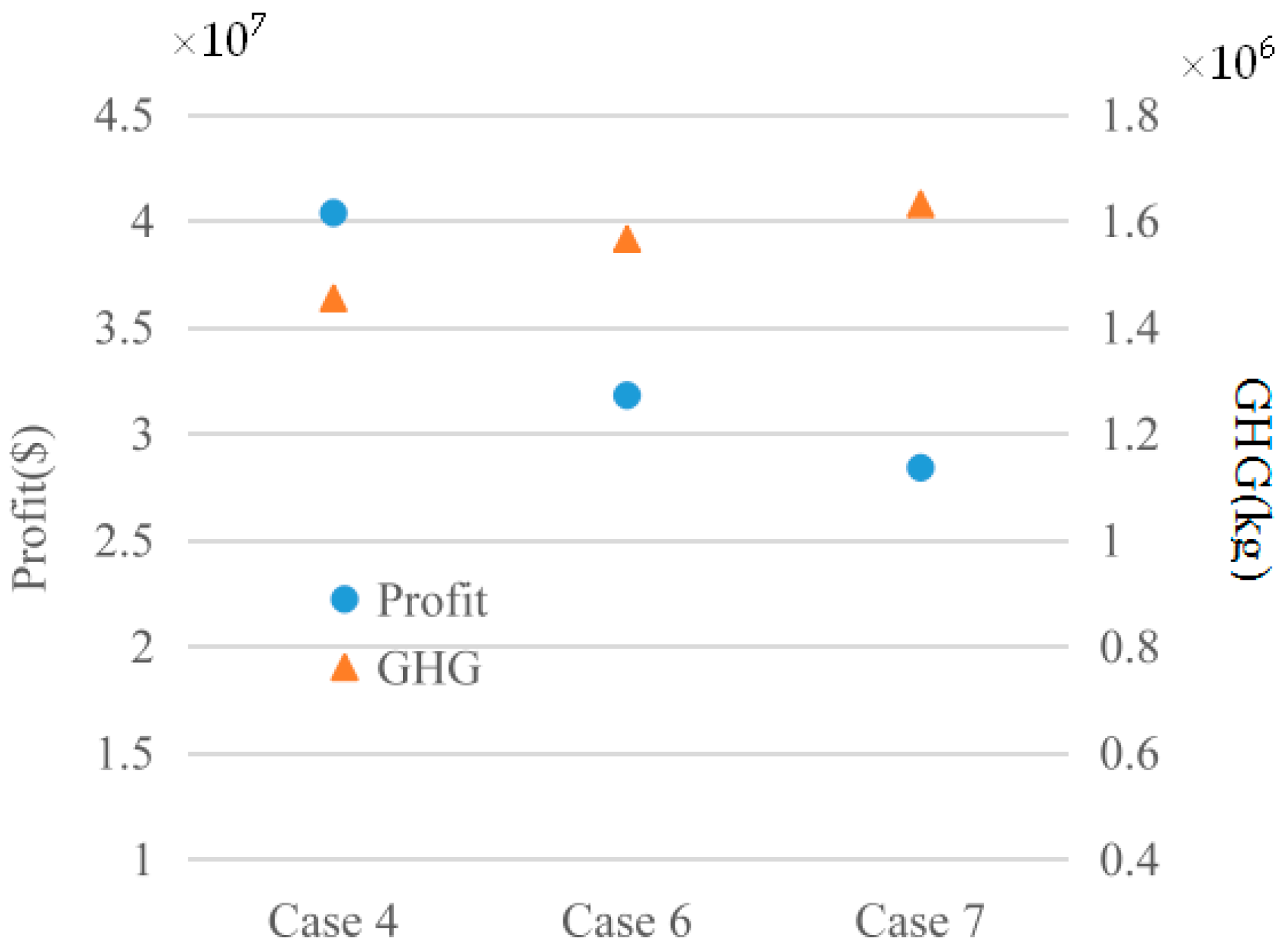
6.3. The Influence of Reliability Threshold Value of a Product on Optimization Results

Case 6: u₁ = 0.5, u₂ = 0.5, R_n = R_r > 0.90; Case 7: u₁ = 0.5, u₂ = 0.5, R_n = R_r > 0.93

The purpose of the experiment is to observe the influence of the setting of reliability threshold value for a product on optimization results. In order to perform the analysis Case 4, Case 6, and Case 7 are designed. The difference among them is the setting of reliability threshold value of a product. The reliability threshold value of a product is increased from Case 4 to Case 7. The design schemes of product family and remanufactured products for Case 6 and Case 7 are shown in

Table 6. The configuration of product family and remanufactured product in Cases 6 and 7.

-	Product	Module Instance Configuration						Launched in Period
		M1	M2	M3	M4	M5	M6	1	2
Case 6	variant 1	4	4	2	3	2	3	Yes	Yes
	variant 2	4	1	3	2	3	3	Yes	Yes
	variant 3	4	1	1	2	1	1	Yes	Yes
	Remanufactured 1	2	4	1r−1	3	1r−1	2	-	Yes
	Remanufactured 2	1	3	1r−1	3	1r−1	2	-	Yes
	Remanufactured 3	1	1r−2	2	2	1	3	-	Yes
Case 7	variant 1	2	3	3	2	3	3	Yes	Yes
	variant 2	3	3	3	2	1	3	Yes	Yes
	variant 3	4	1	1	2	1	1	Yes	Yes
	Remanufactured 1	2	4	1r−1	3	3	2	-	Yes
	Remanufactured 2	3	3	1r−1	3	3	3	-	Yes
	Remanufactured 3	1	1r−1	1	3	1	2	-	Yes

^r−x denotes that a remanufactured component with the xst reliability is configured.

. It can be seen that the design schemes of Case 4, Case 6, and Case 7 are different. For example, both Case 6 and Case 7 select M_2,1 as remanufactured component for configuring remanufactured products, but the selected remanufactured technologies for M_2,1 are different in Cases 6 and 7. This is due to the reliability threshold value of a product in Case 7 is greater than that in Case 6. Moreover, the achieved reliabilities for M_2,1 are different by adopting different remanufactured technology. Therefore, for improving the reliability value of a remanufactured product, different remanufacturing technologies can also be considered to improve the reliability of remanufactured component except selecting new component with high reliability. This proved to be a good choice that the selection of remanufacturing parameters (e.g., selection of remanufacturing technology) is considered in the concurrent planning of product family and remanufactured products for obtaining the effective design schemes. The optimization results are provided in Figure 7. It can be seen that the profit is decreased while GHG emission is increased from Case 4 to Case 7. In Case 4, Case 6, and Case 7, all optimization conditions (including the optimization objectives and the weight of each objective) are the same except for the setting of reliability threshold of products. If the threshold level of product reliability as set is increased under the same other optimization conditions, the results indicate that the profit will be reduced while GHG emission is increasing. This is because more cost and GHG emissions are inevitable to improve the reliability of components. Figure 7 can provide a rough reference for the setting of reliability threshold of products when the weight of GHG emission and the weight of profit are set equal (u₁ = 0.5, u₂ = 0.5). For example, if the environmental regulation restricts the GHG emission to below 1.6 million kilograms, or the expected profit of a company is not less than 25 million dollars, the setting of reliability threshold should not be higher than 0.93 (referenced by Case 7).

7. Conclusions

It is widely accepted that global warming has become one of the biggest environmental concern for human being. Low-carbon product family design is considered as one of the effective measures to reduce GHG emission from product. Nevertheless, current studies on low-carbon product family design do not consider remanufactured products. In recent years, the sales of remanufactured products are increasing due to higher profit for the company and environmental benefits. Since the remanufactured product design is largely influenced by product family design, the product family design and remanufactured product design should be considered simultaneously in order to maximize profits and minimize GHG emission. This paper presented an optimization method for coordinated low-carbon design of product family and remanufactured products. The design of all product variants contained in a low-carbon product family and the plan of remanufactured products are determined concurrently. The genetic algorithm was designed to solve the optimization problem. Finally, the proposed approach was verified by a case study. Experiment results indicate that the two optimization objectives, profit and GHG emission, are contradictory in coordinated low-carbon design of product family and remanufactured products. By investigating the influence of integrated and separated remanufactured product design on low-carbon product family design, the results show that the joint optimization of product family design and remanufactured products planning can bring more profit and less GHG emission comparing with separation optimization. Moreover, by analyzing the reliability threshold value of a product, the result indicates that it affects the GHG emission and profit. Therefore, the reliability threshold value of the product needs to be reasonably set in coordination with the low-carbon design of the product family and remanufactured product. Some insights from the case study are as follows: as an important way to contribute to sustainability, remanufacturing can help the enterprises gain not only economic benefits but also environmental benefits. Since remanufactured products planning is affected by product family design and remanufactured products cannibalize new product sales, remanufactured products need to be planned reasonably for maximum benefit. Compared with sequential design, the concurrent planning of product family and remanufactured products can bring more profit and less GHG emission. In addition, the selection of remanufacturing parameters (e.g., selection of remanufacturing technology) affects the planning of remanufactured products, so then it further affects the product family design. Therefore, it is a very good choice that the selection of remanufacturing parameters is considered in the concurrent planning of product family and remanufactured products for obtaining the effective design schemes.

As future work, it is worthwhile to consider uncertainty in the optimization model. In real world, the customer’s preference may be ambiguous. Moreover, the market demand and the information of competing product may be vague. Therefore, under these uncertain conditions, how to gain a robust solution would be an interesting problem.

References

1. Intergovernmental Panel on Climate Change (IPCC). IPCC Fourth Assessment Report: Climate Change 2007; Cambridge University Press: New York, NY, USA, 2007; pp. 447–496. [Google Scholar]
2. Mascle, C.; Zhao, H.P. Integrating environmental consciousness in product/process development based on life-cycle thinking. Int. J. Prod. Econ. 2008, 112, 5–17. [Google Scholar] [CrossRef]
3. Kengpol, A.; Boonkanit, P. The decision support framework for developing ecodesign at conceptual phase based upon iso/tr 14062. Int. J. Prod. Econ. 2011, 131, 4–14. [Google Scholar] [CrossRef]
4. Ferrer, G.; Swaminathan, J.M. Managing new and differentiated remanufactured products. Eur. J. Oper. Res. 2010, 203, 370–379. [Google Scholar] [CrossRef] [Green Version]
5. Sutherland, J.W.; Adler, D.P.; Haapala, K.R.; Kumar, V. A comparison of manufacturing and remanufacturing energy intensities with application to diesel engine production. CIRP Ann.-Manuf. Technol. 2008, 57, 5–8. [Google Scholar] [CrossRef]
6. Song, J.S.; Lee, K.M. Development of a low-carbon product design system based on embedded GHG emissions. Resour. Conserv. Recycl. 2010, 54, 547–556. [Google Scholar] [CrossRef]
7. Qi, Y.; Wu, X.B. Low-carbon technologies integrated innovation strategy based on modular design. Energy Procedia 2011, 5, 2509–2515. [Google Scholar] [CrossRef]
8. Su, J.C.P.; Chu, C.; Wang, Y. A decision support system to estimate the carbon emission and cost of product designs. Int. J. Precis. Eng. Manuf. 2012, 13, 1037–1045. [Google Scholar] [CrossRef]
9. Kuo, T.C.; Chen, H.M.; Liu, C.Y.; Tu, J.C.; Yeh, T.C. Applying multi-objective planning in low-carbon product design. Int. J. Precis. Eng. Manuf. 2014, 15, 241–249. [Google Scholar] [CrossRef]
10. Xu, Z.Z.; Wang, Y.S.; Teng, Z.R.; Zhong, C.Q.; Teng, H.F. Low-carbon product multi-objective optimization design for meeting requirements of enterprise, user and government. J. Clean. Prod. 2015, 103, 747–758. [Google Scholar] [CrossRef]
11. He, B.; Wang, J.; Huang, S.; Wang, Y. Low-carbon product design for product life cycle. J. Eng. Des. 2015, 26, 321–339. [Google Scholar] [CrossRef]
12. Chiang, T.A.; Che, Z.H. A Decision-Making Methodology for Low-Carbon Electronic Product Design. Decis. Support Syst. 2015, 71, 1–13. [Google Scholar] [CrossRef]
13. He, B.; Tang, W.; Wang, J.; Huang, S.; Deng, Z.Q.; Wang, Y. Low-carbon conceptual design based on product life cycle assessment. Int. J. Adv. Manuf. Technol. 2015, 81, 863–874. [Google Scholar] [CrossRef]
14. Jiao, J.; Simpson, T.W.; Siddique, Z. Product family design and platform-based product development: A state-of-the-art review. J. Intell. Manuf. 2007, 18, 5–29. [Google Scholar] [CrossRef]
15. Francalanza, E.; Borg, J.C.; Constantinescu, C. A case for assisting ’Product Family’ manufacturing system designers. Procedia CIRP 2012, 3, 376–381. [Google Scholar] [CrossRef]
16. Bryan, A.; Wang, H.; Abell, J. Concurrent Design of Product Families and Reconfigurable Assembly Systems. J. Mech. Des. 2013, 135, 051001. [Google Scholar] [CrossRef]
17. Wang, Q.; Tang, D.B.; Yin, L.L.; Salido, M.A.; Giret, A.; Xu, Y.C. Bi-objective optimization for low-carbon product family design. Robot. Comput.-Int. Manuf. 2016, 41, 53–65. [Google Scholar] [CrossRef]
18. Tang, D.B.; Wang, Q.; Ullah, I. Optimisation of product configuration in consideration of customer satisfaction and low carbon. Int. J. Prod. Res. 2017, 55, 3349–3373. [Google Scholar] [CrossRef]
19. Kim, S.; Moon, S.K. Sustainable platform identification for product family design. J. Clean. Prod. 2017, 143, 567–581. [Google Scholar] [CrossRef]
20. Xiao, W.X.; Du, G.; Zhang, Y.Y.; Liu, X.J. Coordinated optimization of low-carbon product family and its manufacturing process design by a bilevel game-theoretic model. J. Clean. Prod. 2018, 184, 754–773. [Google Scholar] [CrossRef]
21. Mangun, D.; Thurston, D.L. Incorporating component reuse, remanufacture, and recycle into product portfolio design. IEEE Trans. Eng. Manag. 2002, 49, 479–490. [Google Scholar] [CrossRef]
22. Debo, L.G.; Toktay, L.B.; Wassenhove, L.N.V. Joint life-cycle dynamics of new and remanufactured products. Prod. Oper. Manag. 2006, 15, 498–513. [Google Scholar] [CrossRef]
23. Vorasayan, J.; Ryan, S.M. Optimal price and quantity of refurbished products. Prod. Oper. Manag. 2006, 15, 369–383. [Google Scholar] [CrossRef]
24. Kwak, M.; Kim, H.M. Assessing product family design from an end-of-life perspective. Eng. Optim. 2011, 43, 233–255. [Google Scholar] [CrossRef]
25. Kwak, M.; Kim, H.M. Market positioning of remanufactured products with optimal planning for part upgrades. J. Mech. Des. 2013, 135, 1–10. [Google Scholar] [CrossRef]
26. Debo, L.G.; Toktay, L.B.; Wassenhove, L.N.V. Market Segmentation and Product Technology Selection for Remanufacturable Products. Manag. Sci. 2005, 51, 1193–1205. [Google Scholar] [CrossRef] [Green Version]
27. Ferguson, M.E.; Toktay, L.B. The Effect of Competition on Recovery Strategies. Prod. Oper. Manag. 2006, 15, 351–368. [Google Scholar] [CrossRef]
28. Jin, Y.; Muriel, A.; Lu, Y. When to Offer Lower Quality or Remanufactured Versions of a Product. Decis. Sci. 2016, 47, 699–719. [Google Scholar] [CrossRef]
29. Liu, B.; Holmbom, M.; Segerstedt, A.; Chen, W. Effects of carbon emission regulations on remanufacturing decisions with limited information of demand distribution. Int. J. Prod. Res. 2015, 53, 532–548. [Google Scholar] [CrossRef]
30. Wang, Y.; Chen, W.; Liu, B. Manufacturing/remanufacturing decisions for a capital-constrained manufacturer considering carbon emission cap and trade. J. Clean. Prod. 2017, 140, 1118–1128. [Google Scholar] [CrossRef]
31. Yenipazarli, A. Managing new and remanufactured products to mitigate environmental damage under emissions regulation. Eur. J. Oper. Res. 2016, 249, 117–130. [Google Scholar] [CrossRef]
32. Simpson, T. A Concept Exploration Method for Product Family Design. Ph.D. Thesis, Georgia Institute of Technology, Atlanta, GA, USA, 1998. [Google Scholar]
33. Perera, H.S.; Nagarur, N.; Tabucanon, M.T. Component part standardization: A way to reduce the life-cycle costs of products. Int. J. Prod. Econ. 1999, 60–61, 109–116. [Google Scholar] [CrossRef]
34. Kwak, M. Green Profit Design for Lifecycle. Ph.D. Thesis, University of Illinois at Urbana-Champaign, Urbana, IL, USA, 2012. [Google Scholar]
35. Hsu, T.H.; Chu, K.M.; Chan, H.C. The fuzzy clustering on market segment. In Proceedings of the IEEE International Conference on Fuzzy Systems, San Antonio, TX, USA, 7–10 May 2000. [Google Scholar]
36. Jiao, J.X.; Zhang, Y. Product portfolio planning with customer-engineering interaction. IIE Trans. 2005, 37, 801–814. [Google Scholar] [CrossRef]
37. Mukhopadhyay, S.K.; Ma, H. Joint procurement and production decisions in remanufacturing under quality and demand uncertainty. Int. J. Prod. Econ. 2009, 120, 5–17. [Google Scholar] [CrossRef]
38. Wang, K.; Choi, S.H. A holonic approach to flexible flow shop scheduling under stochastic processing times. Comput. Oper. Res. 2014, 43, 157–168. [Google Scholar] [CrossRef]
Figure 1. The two periods of launching new products and remanufactured product.
Sustainability 11 00460 g001
Figure 2. An example of a chromosome.
Sustainability 11 00460 g002
Figure 3. An example for crossover operation.
Sustainability 11 00460 g003
Figure 4. The optimization results of Case 1 to Case 4.
Sustainability 11 00460 g004
Figure 5. Identifying the design scheme.
Sustainability 11 00460 g005
Figure 6. (a) The profit in Case 4 and Case 5; and (b) the GHG emission in Case 4 and Case 5.
Sustainability 11 00460 g006
Figure 7. The optimization results of Cases 4–7.
Sustainability 11 00460 g007