An Improved Method for Obtaining Solar Irradiation Data at Temporal High-Resolution

Abstract

Solar irradiation that is received on a terrestrial surface at minor scale of an hour does not have many records, since the current solar irradiation databases generally only have data recorded on a daily (most) and hourly (some less) scale. For places where there are no records of solar irradiation, there are a lot of methods that are used to synthetically or artificially generate these data, and again they are usually methods that generate data on a daily or hourly scale. Currently, for all types of applications, especially in the field of photovoltaic solar energy, irradiation data are needed at minor scale of an hour. In this case, there are very few methods to generate such data. For this purpose, a new methodology to generate series of solar irradiation at temporal high-resolution. In this paper, it is presented on a 10-min basis. A comparative study with real data has been done and the conclusion, as it will be explained is that the proposed methodology provides very good results.

1. Introduction

The adequate knowledge of the solar irradiation is the starting point for all types of applications in the field of renewable energy in general and photovoltaic (PV now on) solar energy in particular [1]. The two main characteristics of solar irradiation are low density and variability over time. Both characteristics are fundamental when it comes to knowing how much energy from the sun can be used. There are several procedures and methodologies to obtain solar irradiation: measured with different instruments [2,3,4], consult solar irradiation data bases and satellite images [5], or generation of synthetical series of solar irradiation [6,7]. There are mainly two time scales in which the studies on solar characterization have been well developed and studied: daily solar irradiation series and hourly solar irradiation series. However, for shorter time scales, the proposal of current prediction methods to generate series of solar irradiation is usually quite complex and very local. This is because the variability that solar irradiation presents at shorter time scales (lower than an hour) is complex and difficult to determine.

With the development of advanced energy services in smart microgrids (e.g., households with PV distributed generation, hereafter household-prosumers), it is very important to lower the time scale for the availability of solar irradiation data. Thus, data that are going to be needed are instantaneous solar irradiation data, or on time scales of the order of a few seconds to minutes. The range of services provided include the application of demand response measures [8,9,10,11,12,13,14], smart home/building automation [15,16,17], and the provision of balancing services, such as frequency control services (frequency containment reserve [18,19,20,21,22] and frequency restoration reserve [23]). The design of these services is based on the training and validation of models, which requires temporal high-resolution data for generation/load profiles. The optimal sizing of storage and generation facilities for these household-prosumers [10,24,25,26,27] also depends on the availability of reliable generation/load profile data. The criteria for this sizing are based on technical, economical, and hybrid indicators [28]. Not surprisingly, the monitoring of household generation/load profiles has experienced an exponential growth in recent years [29,30,31]. In fact, many of the electricity distribution companies carry out the installation of smart meters for the remote reading of electrical consumption.

Smart grids must realize the “smart cities” that are an emerging paradigm throughout the world. “Smart cities” are supported by studies on the energy behavior of cities around the world. Such is the scope of the issue that the European Commission, in its draft proposals for the imminent call of the Horizon 2020 program, points to Smart Green as a priority action line. As previously mentioned, methods that synthetically generate solar irradiation data at daily and hourly scales have been well studied and contrasted. The next section summarizes some of them, highlighting its main features. Nevertheless, for less than the hour values of solar irradiation data, there are few works nowadays. This is the reason that it is a very important field of researching, and its applications will be very important.

The objective of this work is to present a methodology for predicting solar irradiation at a lower scale of the hour.

The structure of this paper is the following. In this first section, the introduction to the paper is presented plus. Section two is the materials and methods used in this work. In this section, a review of the most important methods for predicting solar irradiation and an explanation of the database used and the methodology that was proposed is developed. In Section three, the results are presented. Finally, the discussion and conclusion are included in Section four and five.

2. Materials and Methods

2.1. Methods for Predicting Solar Irradiation

In order to have long sequences of solar irradiation, here are lots of methods for obtaining solar irradiation at different time scales. The two main scales where most authors have presented methods or methodologies for generating what is named “synthetic solar irradiation data” are daily scale and hourly scale.

In all of these methods, the underlying idea can be summarized as starting from an exhaustive statistical study of the historical records of the locality or localities for which solar data are available, to later propose a mathematical model of generation solar. In this statistical study of the data, at least the following two types of characteristics must be included:

• Independent characteristics of solar irradiation time, such as means (both monthly and annual), variances, or standard deviations, etc.
• Time-dependent or sequential characteristics of solar irradiation: mainly partial and total autocorrelation functions.

Once these parameters are known, the next step is the proposal of a mathematical model that generates synthetic irradiation series that are equivalent to the real series, in the sense that the aforementioned statistical parameters must be similar (the closer the better) to the values of the real series, within certain reliability margins.

Hereafter, a review of the methods of generating series on a daily scale is firstly presented and then those of the hourly scales.

One of the pioneering works in the field of daily series was due to Klein [32]. This researcher made use of the fact that most of the seasonal variations of the global daily irradiation were due to variations in the extraterrestrial or extra atmospheric irradiation (the one that affects the upper layers of the Earth, without having managed to cross the atmosphere), and these seasonal variations can be eliminated while using the K_T clarity index (quotient between global irradiation and extraterrestrial irradiation) as a variable. In this way, the variable to be modeled was not the global irradiation itself but the index of clarity. However, many other researchers began studying the global irradiation itself.

Thus, Brinkworth carried out another of the first works [33] while using an autoregressive model with moving average (ARMA: AutoRegressive Moving Average) applied directly on the daily global irradiation data. Paasen [34] modeled the daily irradiation sequences in the Netherlands, while using a modified irradiation variable. Exell [35] and Vergara-Domínguez et al. [36] made use of a new variable, called clear sky irradiation, which is similar to the clarity index. However, none of these authors incorporated in their study the analysis of the distribution of the data obtained by means of the distribution function. In this sense, Amato et al. [37] included the distribution function of the daily global irradiation series, but, nevertheless, the proposed model was only applicable to the locality under study, that is, it was not of universal application.

Although the global irradiation distribution function will locally depend on where the irradiation comes from, Liu and Jordan [38] showed that, for the case of the distribution functions of the daily clarity index, they are universal. In addition, these functions are non-Gaussian, dependent on the monthly clarity index, and therefore monthly variables. Dagelman carried out a work that already included the universal distribution functions of Liu and Jordan [39], who proposed a method for generating the daily clarity indices in a random way from the distribution curves of Liu and Jordan.

Also important are the works of Boileau [40], based on developments in Fourier series, and those of Bartoli et al. [41] also focused on Fourier series and Markov processes. However, the most widespread are those that were proposed by Graham and Hollands [42] based on Gaussian inversion techniques and those of Aguiar and Collares-Pereira [43] that makes use of Markov Transition Matrices. These last two works are currently considered the best in this field, and they are usually used as a basis to generate artificial sequences of solar irradiation with great rigor. In the case of Graham and Hollands, the study was conducted with Canadian localities from different climates, and in the case of Aguiar, the locations used were from several countries, from Portugal to Macao (China).

Regarding hourly generation methods, one of the pioneering works based on ARMA processes was due to Goh and Tan [44] for data from Singapore. Mustacchi et al. [45], studying about twenty Italian localities, used Markov Transition Matrices to simulate the stochastic processes that were implicit in the real time solar irradiation series. A method that was based on spectral techniques was presented by Balouktsis and Tsalides [46] for data from Athens. The Spanish researchers Llanos Mora and Mariano Sidrach [47] present a model that was based on multiplicative ARMA processes, while using data from Spanish localities, while Palomo [48], also for Spanish localities, uses Markov transition matrices.

However, once again, the methods that were used as a paradigm in this field are again those that were proposed by Graham and Hollands [49] and by Aguiar and Collares-Pereira [50]. The method presented by Graham and Hollands makes use of ARMA and Gaussian investment processes, being practically a continuation of the work presented for the generation of daily series. However, the work of Aguiar and Collares-Pereira is quite different from the one that they proposed for daily series, since they do not use Markov matrices, but in this case they start by making a very exhaustive study of the data that they have available, discovering certain properties that they try to implement in their new method. This new method is called the Gaussian autoregressive time-dependent model (“TAG: Time dependent Autoregressive Gaussian model”), and the results that it produces are very satisfactorily adjusted to the real hourly solar irradiation values.

It is very important to try to generate solar irradiation data at lower time scales of the hour, as, for instance, in the application of photovoltaic design for smart grids, the data provided by the grid are obtained for minutes or even less. Nevertheless, for lower time scales (less than an hour), there are few works [30,31,32]. A bibliographic search has been done and it can be summarized as the most relevant.

In 2009, Reikard [51] presented a work in which he analyzes different methods to make predictions about the behavior of solar irradiation in two possible time scales: (a) time slots (intervals of 1 h, 2 h, 3 h, and 4 h) and (b) minutes (intervals of 5 min, 15 min, 30 min, and 60 min). It is interesting to note that, already in this work, authors present a study that goes down to the scale of minutes to predict solar irradiation. Of the six methods analyzed, it concludes that for hour forecasts the best method is one that is based on ARIMA (AutoRegressive Integrated Moving Average) methods, methods that are fully contrasted by many other researchers. For periods of minutes, the ARIMA method is still almost the best, although it is slightly surpassed with a methodology that is based on Neural Networks, especially for periods of 5 min, although when the interval is greater, it continues to dominate the ARIMA method.

Additionally, Barbieri et al. [52], presented a work in which on the one hand explains how to make the possible prediction of the PV power of a PV system from solar irradiation prediction methods (also for wind) in the very short term and by another side makes an important revision of solar irradiation methods. In this case, he concludes that the most reliable methods are those that are based on neural networks to predict solar irradiation. Despite all of these researchers insisting on the difficulty of predicting the output of a PV system in the short term due to the difficulty of the previous prediction in solar irradiation, the methodology proposed could be very interesting to reproduce in our characterization.

Rahmann et al. [53] propose a method of control strategy to reduce the impacts on long-term PV plants, when fluctuations occur in the input (solar irradiation). It proposes methods for the prediction of solar irradiation on the daily scale while using finally three typical days: sunny (clear), partly cloudy, and totally cloudy and the methodology of Neural Networks.

Finally, it is interesting to highlight the work, as previously mentioned, done by Mora et al. [47], in which they propose an ARMA method for the generation of solar irradiation data at a time scale. It is one of the methods that gives better results, so its reproducibility at a minor time scale of an hour can be analyzed.

The first conclusion that can be drawn from the literature review is that there are methods for the generation of solar irradiation at a time scale that are highly contrasted and mainly based on two major types, those that are based on classical methods, such as ARIMA and ARMA, and those that are based on newer methods, such as artificial neural networks. However, there are not many methods for predicting solar irradiation at a minor time scale of an hour. Nowadays, studies and the proposal of methods to generate solar irradiation series are increasing. These methods are usually quite complex and very local, since the variability that solar irradiation presents at minor time scale of an hour is complex and difficult to determine. This is where there is a wide study field that authors try to cover.

2.2. Database of Solar Irradiation in Jaén

The initial material available is a database of solar irradiation available in Jaén. (Spain, latitude 37.73° N, 3.73° W), where we have our research laboratory and a solar irradiation data base of many years. The accessible data are values of solar irradiation at a minor time scale of an hour (values every 10 min). Our research group has been recording solar irradiation data in the city of Jaén from 1996 to 2003 and from 2005 to 2011, in a time scale of 10 min.

Subsequently, these data have been sorted and filtered in order to eliminate errors. The data measured and provided by the University of Jaén during the study period (from 1996 to 2011, excluding the year 2004) in some cases they were null, which will be called erroneous. For this reason, a filtering of said values has been carried out in order to obtain a more complete database.

For this, a previous study of ordering and detection of errors was carried out.

Table 1. Days under study.

Period	Total Days	Days with Errors	Percentage of Days with Errors
1996–2011	5476	250	4.56%

shows the errors that were detected and the percentage of final error.

Finally, a database of more than 15 years has been obtained, with data at minor time scale of an hour: approximately 788,400 data.

This database was already characterized and the Typical Meteorological Year (TMY) [54] was obtained. In next two sections, we explain the characterization done and the calculation of the TMY.

2.3. Characterization of Solar Irradiation in Jaén

Once the database is available, the characterization of the hourly solar irradiation has been carried out. The fundamental parameters that are necessary for a correct solar characterization have been calculated, such as mean values, variances, and distribution functions. The knowledge of these parameters allows for making adjustments of the coefficients of solar irradiation generation methods, such as the ARIMA methods.

A series of statistical parameters have been calculated to characterize solar irradiation, such as means and standard deviations. Additionally, a good characterization involves knowing the main components of solar irradiation (direct, diffuse, and albedo), as well as certain relationships between them, such as the clarity index ($K_T$) or the diffuse fraction ($K_D$). In the following section, the most important parameters that were carried out in this characterization are shown.

2.4. Calculation of the Typical Meteorological Year (TMY) for Jaén

Finally, the Typical Meteorological Year (TMY) has been calculated to complete the characterization of solar irradiation in Jaén. The main function of the TMY is to be able to perform simulations in the case of not having a method to generate solar irradiation series, since the TMY works the same as any series generated. A TMY internally conserves the parameters and fundamental characteristics of the solar irradiation of a certain place.

By definition, a TMY is one that collects the different hourly values of global horizontal irradiation and ambient temperature obtained over a hypothetical year constituted by a succession of twelve months belonging to a set of real years. These twelve months are chosen, so that the TMY represents with reliability the meteorological characteristics of the place in question.

TMY is only available for very few locations, even it is difficult to obtain the hourly values of horizontal irradiation and room temperature for most places.

For the construction of the TMY, different base periods can be used, although it is convenient that this period is the month, that is, it is used, for each generic month that will make up the TMY, all of the data of a single month of the locality in question. Thus, the TMY will represent both the variation of monthly averages throughout the year and the distribution of daily and hourly values within each month.

If the irradiation data of a single year were chosen as a typical year, this would not take into account neither the distribution nor the sequences of the irradiation in this period; otherwise, if they were chosen, for each generic day of a typical year, the data of the actual days would have a succession of days of almost uniform clarity index.

Two different criteria have been used for the selection of the months that will constitute the TMY of the town of Jaén under study:

• Criterion I: Criterion of the monthly average values of daily irradiation.
  Based on finding a month whose average daily irradiation value is as close as possible to the average irradiation value of the same month of all years.
• Criterion II: Criteria for the monthly distribution of values of the clarity index.

For this criterion, a similar study is carried out but with the monthly distribution of the values of the clarity index. In this case, to achieve the appropriate adjustment, a test of goodness of fit must be used; in this case, it has been done following the Kolmogorov–Smirnov test [55]. This test involves the examination of a random sample (that will have some unknown distribution) versus a known distribution function.

The Kolmogorov–Smirnov test for a sample is a “goodness of fit” procedure, which allows for measuring the degree of agreement between the distribution of a data set and a specific theoretical distribution. Its objective is to indicate whether the data come from a population that has the specified theoretical distribution, that is, it contrasts if the observations could reasonably come from the specified distribution.

The Kolmogorov–Smirnov test has been used to locate the degree of similarity that exists between the distribution function in a month and that of the generic distribution function.

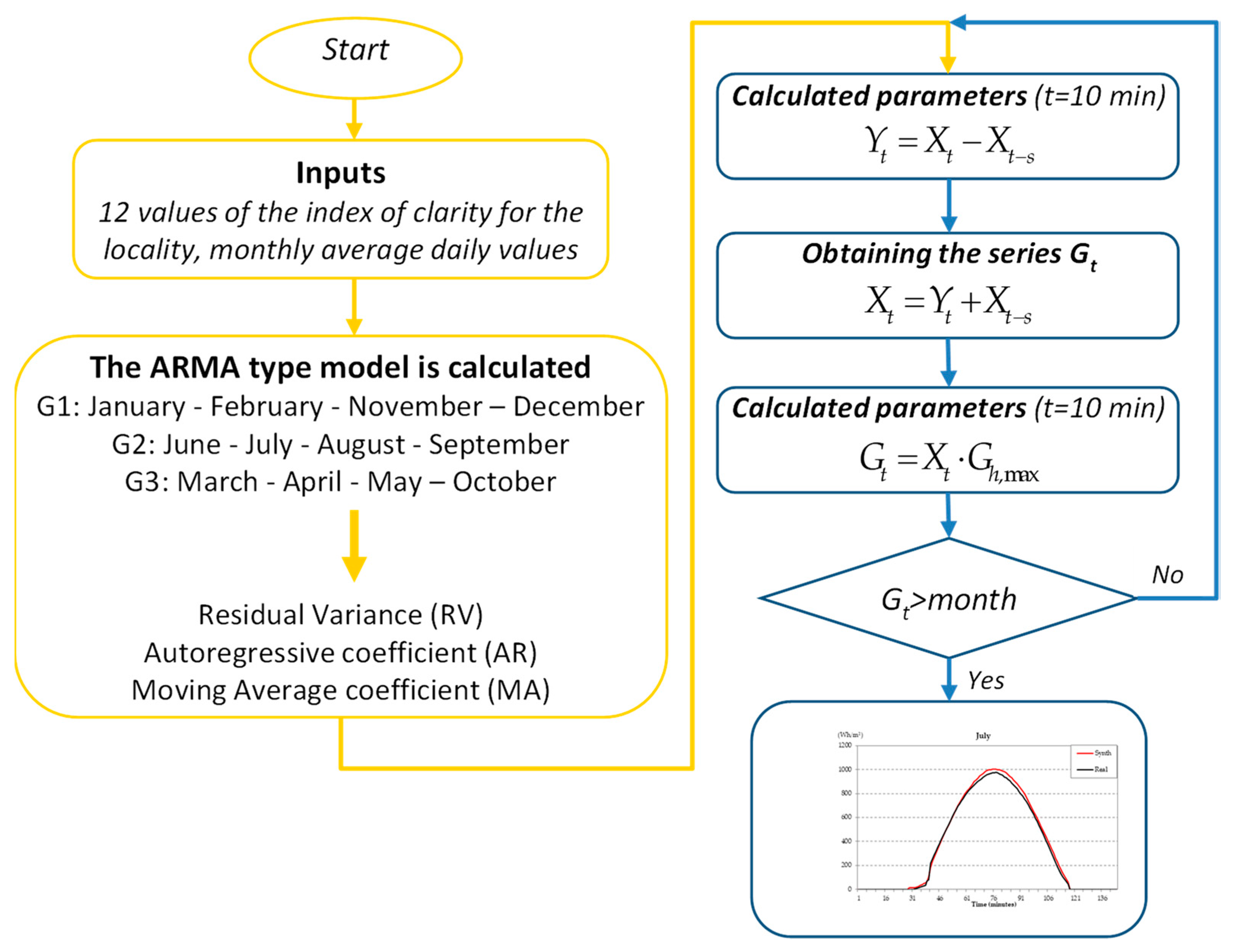
2.5. Proposed Method to Generate Data of Solar Irradiation at Minor Time Scale of an Hour

From the revised methods, it is considered that one of the best methods for generating synthetic solar irradiation series is the one proposed by Mora-Sidrach. Based on this method, the authors have adapted it to the data of the locality under study and a method to generate solar irradiation series at the 10-min scale is proposed. Figure 1 shows a flowchart of the proposed method.

• Step 1: One should start from knowing 12 values of the index of clarity for the locality, in particular of the twelve monthly average daily values of said index.
  The expression for this first variable is given by:

  $$K_{tm}=\frac{G_{dm}}{B_{odm}}$$

  (1)

  where:
  $K_{tm}$: monthly average daily clarity index
  $G_{dm}$: monthly average global solar irradiation per month
  $B_{odm}$: monthly average extraterrestrial solar irradiation
  Table 2. Values of $K_{tm}$ from the typical meteorological year, location of Jaén.

  Month	${\mathit{K}}_{\mathit{t}\mathit{m}}$
  January	0.481
  February	0.562
  March	0.567
  April	0.575
  May	0.577
  June	0.661
  July	0.676
  August	0.657
  September	0.581
  October	0.577
  November	0.519
  December	0.474

  shows the values of $K_{tm}$ from the typical meteorological year of Jaén.
• Step 2: Determination of the ARMA type model.

Mora and Sidrach proposed several ARMA models, in the sense that, for each model, there are different coefficient for the Residual Variance (RV), Autoregressive coefficient (AR), and Moving Average coefficient (MA). Following similar criterion, but adapted at the Jaén solar irradiation data, five types of ARMA model have been obtained and are included in

Table 3. Values of K_tm for each month to determine the AutoRegressive Moving Average (ARMA) type model.

Model	G1 (group1)January–February–November–December	G2 (group2)June–July–August–September	G3 (group3)March–April–May–October
Type 1	0.583	0.633	0.637
Type 2	0.564	0.614	0.618
Type 3	0.545	0.594	0.598
Type 4	0.514	0.563	0.567
Type 5	0.480	0.530	0.534

. The procedure to determine which type of model has to be applied in each case is as follows. Firstly, the $K_{tm}$ value of the month is used where it included the day where the synthetic series of solar irradiation is going to be generated. The $K_{tm}$ value can be seen in Table 2. With this value Table 3 is consulted to determine the ARMA type model that should be used. In Table 3, there are three variables, G1, G2, and G3, which indicate the group of the month where the calculation of the series is taking place. The corresponding month of each group are:

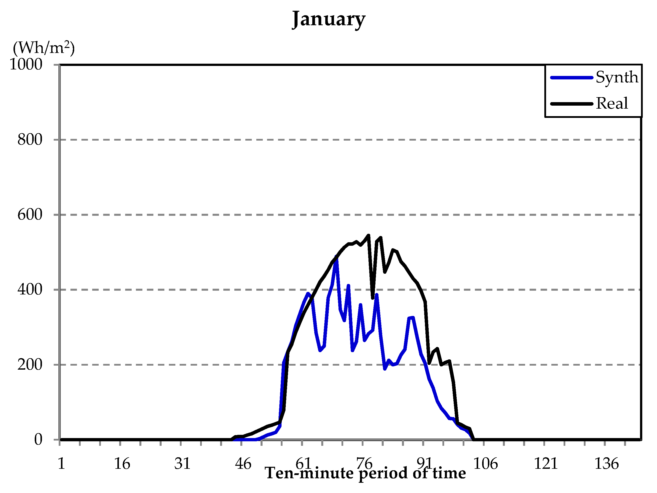
• G1: January–February–November–December
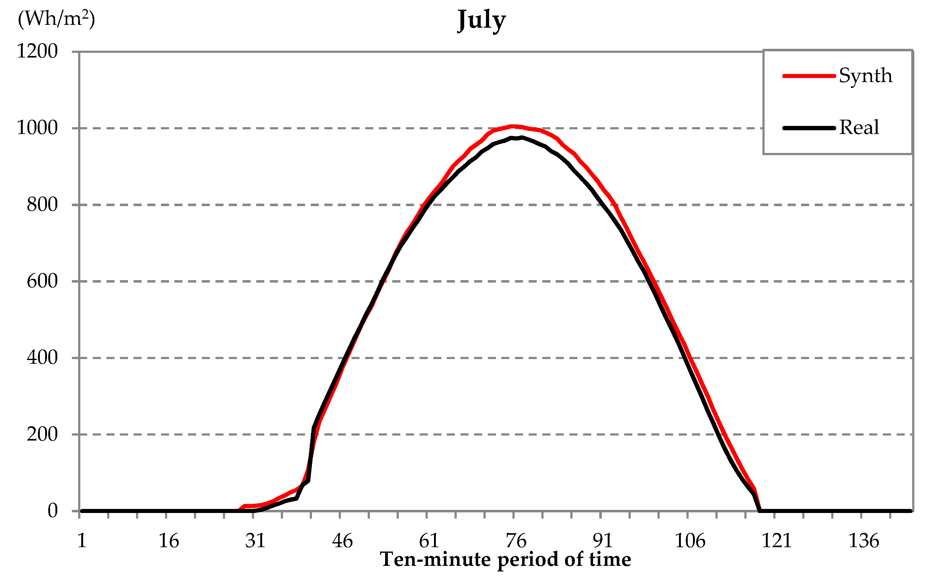
• G2: June–July–August–September
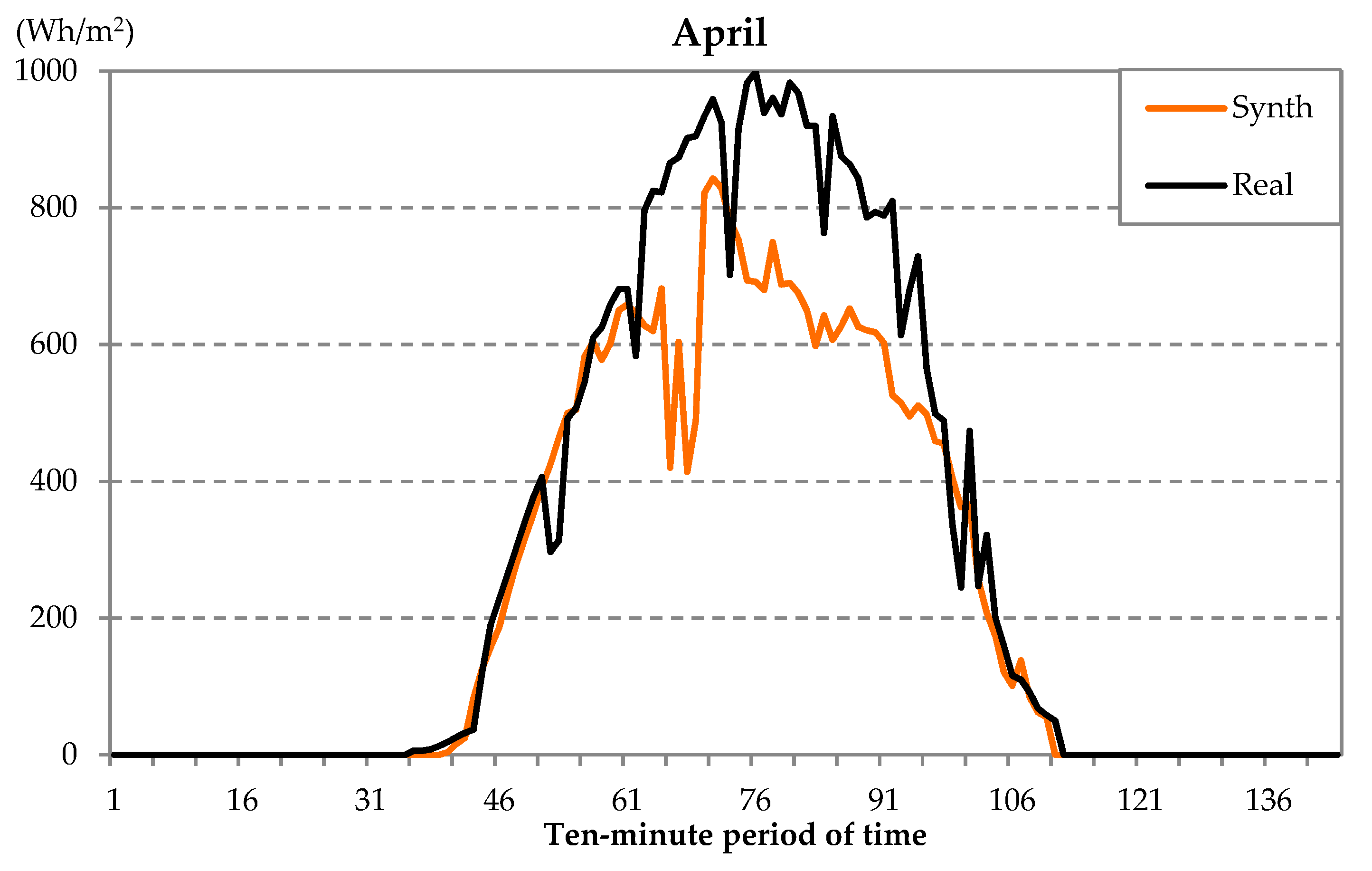
• G3: March–April–May–October

The value of $K_{tm}$ nearest of the values of the columns in Table 3 will indicate the ARMA type model.

Once the ARMA type model is determined, the AutoRegressive coefficient (AR), the Moving Average coefficient (MA), and the Residual Variance coefficient (RV) are indicated in

Table 4. Values of the three main coefficient: Residual Variance (RV), AutoRegressive coefficient (AR), and Moving Average coefficient (MA) for each type of model.

Model	RV	AR	MA
Type 1	0.008	0.720	0.845
Type 2	0.012	0.745	0.845
Type 3	0.018	0.745	0.845
Type 4	0.025	0.762	0.845
Type 5	0.036	0.728	0.862

.

• Step 3: Generation of the series $Y_t$.
  The variable $Y_t$ is defined as:

  $$Y_t=X_t-X_{t-s}$$

  (2)
  The value t indicates a fixed hour, and s is some time before.
  For obtaining $Y_t$ the ARMA model is applied in this way:

  $$Y_t=\mathit{AR}\cdot Y_{t-1}-\mathit{MA}\cdot a_{t-1}+a_t$$

  (3)

  where $a_t$ and $a_{t-s}$ are Gaussian white noise.
• Step 4: Obtaining the series $X_t$.
  In this step, the series $X_t$ is obtained from the previous equation in this way:

  $$X_t=Y_t+X_{t-s}$$

  (4)
• Step 5: Obtaining the series $G_t$.
  $G_t$ is calculated as follows:

  $$G_t=X_t\cdot G_{h,\max }$$

  (5)

  with $G_t=X_t\cdot G_{h,\max }=1100\cdot {\left(\sin \left(\gamma \right)\right)}^{1.05}$ and $\gamma$ is the solar altitude.

3. Results

This section shows the results of the proposed method, mainly via some graphics that underline the synthetical days generated. For instance, in Figure 2, Figure 3 and Figure 4, three typical days of the three groups (G1, G2, and G3) have been included. Figure 2 shows a typical day from group G1 (in this case January). As it can be observed, a real day had a similar evolution as a day synthetically generated from our method, with the difference that the method includes a more pronounced influence of the random component, as usually the days were cloudy in January.

Similarly, in Figure 3, the global solar irradiation evolution on typical April days, one real day and one synthetic days were compared. In this case, in the location in study, April days had values higher than in January, but there were days with some intervals of clouds, which can be seen in Figure 3.

Finally, real days versus synthetic days for July are shown in Figure 4. In this case, it can be observed that this typical days were very sunny (clear days), so the values of the solar irradiation were the highest of the year.

In order to compare qualitatively the data in Figure 2, Figure 3 and Figure 4, A parameter called relative mean variance (RMV) is used:

$$RMV=\frac{{\displaystyle \sum {\left(G_{h-real}-G_{h-synth}\right)}^2}}{{\displaystyle \sum {\left(G_{h-real}-G_{h-mean}\right)}^2}}$$

(6)

where:

$G_{h-real}$: Solar global irradiation real 10 min values

$G_{h-synth}$: Solar global irradiation synthetic 10 min values

$G_{h-mean}$: Solar global irradiation mean value (from real values)

The results of RMV for Figure 2, Figure 3 and Figure 4 are shown in

Table 5. RMV for each representative day analyzed.

Example Day	RMV (%)
January	1.79
April	0.61
July	0.07

.

Table 5 underlines the differences between the two series, the one obtained synthetical and the real data for the three days.

More examples of the evolution of global irradiation are shown in Figure 5, Figure 6 and Figure 7, where ten days for the three types of groups were generated. In this case, the same months have been chosen, i.e., January, April, and July.

It can be observed that the evolution of the global solar irradiation had a random component that was more influenced on January or April (more cloudy days) than in July (clear days).

Finally, the variable RMV for the whole year generated synthetical and compared with a real year is shown in

Table 6. RMV for a representative month of each group (G1, G2, and G3).

Example Day	RMV (%)
January (G1)	2.37
April (G3)	1.13
July (G2)	0.16

.

The RMV value for the whole year was 4.15%.

4. Discussion

After analyzing the results in the previous section, the graphs of the days that were generated in a synthetic way, as well as the tables with the errors observed between the real data and the synthetic data, the proposed method is very useful for obtaining solar irradiation data at a minor time scale of an hour.

It has to be said that, when the day is sunny, the method is highly effective. The differences between the days of solar irradiation generated synthetically, as compared to the days of real solar irradiation are indistinguishable. However, for cloudy days, the differences between the types of days are greater. This is totally logical and justifiable, since the random component that is associated with the evolution of solar irradiation, due mainly the influence of clouds, is higher for cloudy days. This leads to a method in this case somewhat less effective. On the contrary, for clear days, as indicated and can be seen in the results, the method works correctly.

In any case, it should be noted that, for the locations with climates similar to the locality in the study, where the clear days predominate, the method works correctly.

As for the errors, we conclude that, for days of the group G2, the error is less than 1%, for Groups G1 and G3, the error is less than 3%, and the error for a complete synthetical year is less than 5%.

5. Conclusions

As final conclusions, it would be interesting to highlight the following. Firstly, it is necessary to emphasize that this work has begun carrying out an exhaustive work of bibliographical search on methods that serve to generate solar irradiation at minor time scale of an hour. It was found that there is not much literature on the subject, although it is a very interesting field of study for future applications that may be in the PV field.

Secondly, it can be concluded that a very reliable method has been presented to generate sequences of solar irradiation in a synthetic way. From the results that were obtained, it works correctly. In the operation of the developed method, it is necessary to clearly distinguish between cloudy days and clear days, among which there is a difference in the operation of the method used.

Hence, for clear days, it is observed that the method works properly, as can be observed from the results obtained. In these cases, the errors are less than 0.1%, and it can be said that the days artificially generated by the proposed method and the real days used to compare are practically indistinguishable. However, for cloudy days, there are somewhat greater differences between artificial and real days. As a future investigation, we would like to improve the generation of cloudy days.

Another conclusion is that this type of study is only applicable in this case for locations with climates that are similar to the locality under study. The authors cannot categorically claim that it can be extrapolated to other locations. We think that, in this sense, the extension of this methodology to other places will require the adjustment of the fundamental ARMA parameters, with which this situation could be considered as a possible future line of study. Therefore, this work is only a first step towards obtaining a method that is universal for other locations, although the methodology could be reproducible in different places, simply by making a preliminary study of the solar irradiation available in order to adjust the mentioned parameters.

References

1. Jiménez-Torres, M.; Rus-Casas, C.; Lemus-Zúñiga, L.G.; Hontoria, L. The importance of accurate solar data for designing solar photovoltaic systems—Case studies in Spain. Sustainability 2017, 9, 247. [Google Scholar] [CrossRef]
2. Rus-Casas, C.; Hontoria, L.; Fernández-Carrasco, J.I.; Jiménez-Castillo, G.; Muñoz-Rodríguez, F. Development of a utility model for the measurement of global irradiation in photovoltaic applications in the internet of things (IoT). Electronics 2019, 8, 30. [Google Scholar] [CrossRef]
3. López-Lapeña, O.; Pallas-Areny, R. Solar energy irradiation measurement with a low–power solar energy harvester. Comput. Electron. Agric. 2018, 151, 150–155. [Google Scholar] [CrossRef]
4. Rus-Casas, C.; Aguilar, J.D.; Rodrigo, P.; Almonacid, F.; Pérez-Higueras, P.J. Classification of methods for annual energy harvesting calculations of photovoltaic generators. Energy Convers. Manag. 2014, 78, 527–536. [Google Scholar] [CrossRef]
5. Gueymard, C.A.; Wilcox, S.M. Assessment of spatial and temporal variability in the US solar resource from radiometric measurements and predictions from models using ground-based or satellite data. Sol. Energy 2011, 85, 1068–1084. [Google Scholar] [CrossRef]
6. Hontoria, L.; Aguilera, J.; Zufíria, P. Generation of hourly irirradiation synthetic series using the neural network multilayer perceptron. Sol. Energy 2002, 72, 441–446. [Google Scholar] [CrossRef]
7. Amrouche, B.; Le Pivert, X. Artificial neural network based daily local forecasting for global solar irradiation. Appl. Energy 2014, 130, 333–341. [Google Scholar] [CrossRef]
8. Elma, O.; Tascıkaraglu, A.; Ince, A.T.; Selamogulları, U.S. Implementation of a dynamic energy management system using real time pricing and local renewable energy generation forecasts. Energy 2017, 134, 206–220. [Google Scholar] [CrossRef]
9. Hosseinnia, H.; Tousi, B. Optimal operation of DG-based micro grid (MG) by considering demand response program (DRP). Electr. Power Syst. Res. 2019, 167, 252–260. [Google Scholar] [CrossRef]
10. Oprea, S.V.; Bara, A.; Ileana Uță, A.; Pirjan, A.; Căruțașu, G. Analyses of distributed generation and storage effect on the electricity consumption curve in the smart grid context. Sustainability 2018, 10, 2264. [Google Scholar] [CrossRef]
11. Morales-Velazquez, L.; Romero-Troncoso, R.J.; Herrera-Ruiz, G.; Morinigo-Sotelo, D.; Osornio-Rios, R.A. Smart sensor network for power quality monitoring in electrical installations. Measurement 2017, 103, 133–142. [Google Scholar] [CrossRef]
12. Angrisani, L.; Bonavolonta, F.; Liccardo, A.; Schiano Lo Moriello, R.; Serino, F. Smart power meters in augmented reality environment for electricity consumption awareness. Energies 2018, 11, 2303. [Google Scholar] [CrossRef]
13. Viciana, E.; Alcayde, A.; Montoya, F.G.; Baños, R.; Arrabal-Campos, F.M.; Zapata-Sierra, A.; Manzano-Agugliaro, F. OpenZmeter: An efficient low-cost energy smart meter and power quality analyser. Sustainability 2018, 10, 4038. [Google Scholar] [CrossRef]
14. Sanchez-Sutil, F.; Cano-Ortega, A.; Hernandez, J.C.; Rus-Casas, C. Development and calibration of an open source, low-cost power smart meter prototype for PV household-prosumers. Electronics 2019, 8, 878. [Google Scholar] [CrossRef]
15. Robles Algarín, C.; Sevilla Hernández, D.; Restrepo Leal, D. A low-cost maximum power point tracking system based on neural network inverse model controller. Electronics 2018, 7, 4. [Google Scholar] [CrossRef]
16. Hernández, J.C.; Sanchez-Sutil, F.; Muñoz-Rodríguez, F.J. Design criteria for the optimal sizing of a hybrid energy storage system in PV household-prosumers to maximize self-consumption and self-sufficiency. Energy 2019, 186. [Google Scholar] [CrossRef]
17. Abate, F.; Carratu, M.; Liguori, C.; Paciello, V. A low cost smart power meter for IoT. Measurement 2019, 136, 59–66. [Google Scholar] [CrossRef]
18. Schlund, J.; German, R. A control algorithm for a heterogeneous virtual battery storage providing FCR power. In Proceedings of the 2017 IEEE International Conference on Smart Grid and Smart Cities, Singapore, 23–26 July 2017; pp. 61–66. [Google Scholar] [CrossRef]
19. Megel, O.; Mathieu, J.; Andersson, G. Scheduling distributed energy storage units to provide multiple services. In Proceedings of the IEEE Power Systems Computation Conference, Wroclaw, Poland, 18–22 August 2014; pp. 1–7. [Google Scholar] [CrossRef]
20. Steber, D.; Bazan, P.; German, R. SWARM—Strategies for providing frequency containment reserve power with a distributed battery storage system. In Proceedings of the IEEE International Energy Conference, Leuven, Belgium, 4–8 April 2016; pp. 1–7. [Google Scholar] [CrossRef]
21. Hernandez, J.C.; Sanchez-Sutil, F.; Vidal, P.G.; Rus-Casas, C. Primary frequency control and dynamic grid support for vehicle-to-grid in transmission systems. Int. J. Electr. Power Energy Syst. 2018, 100, 152–166. [Google Scholar] [CrossRef]
22. Hernandez, J.C.; Bueno, P.G.; Sanchez-Sutil, F. Enhanced utility-scale photovoltaic units with frequency support functions and dynamic grid support for transmission systems. IET Renew. Power Gener. 2017, 11, 361–372. [Google Scholar] [CrossRef]
23. Litjens, G.B.M.A.; Worrell, E.; Van Sark, W.G.J.H.M. Economic benefits of combining selfconsumption enhancement with frequency restoration reserves provision by photovoltaic-battery systems. Appl. Energy 2018, 223, 172–187. [Google Scholar] [CrossRef]
24. Braun, M.; Büdenbender, K.; Magnor, D.; Jossen, A. Photovoltaic self-consumption in Germany: Using lithium-ion storage to increase self-consumed photovoltaic energy. In Proceedings of the 24th European Photovoltaic Solar Energy Conference, Hamburg, Germany, 21–24 September 2009; pp. 1–7. [Google Scholar]
25. Bruch, M.; Müller, M. Calculation of the cost-effectiveness of a PV battery system. Energy Procedia 2014, 46, 262–270. [Google Scholar] [CrossRef]
26. Schreiber, M.; Hochloff, P. Capacity-dependent tariffs and residential energy management for PV storage systems. In Proceedings of the IEEE Power and Energy Society General Meeting, Vancouver, BC, Canada, 21–25 July 2013; pp. 1–5. [Google Scholar] [CrossRef]
27. Linssen, J.; Stenzel, P.; Fleer, J. Techno-economic analysis of photovoltaic battery systems and the influence of different consumer load profiles. Appl. Energy 2017, 185, 2019–2025. [Google Scholar] [CrossRef]
28. Luthander, R.; Widen, J.; Nilsson, D.; Palm, J. Photovoltaic self-consumption in buildings: A review. Appl. Energy 2015, 142, 80–94. [Google Scholar] [CrossRef] [Green Version]
29. Fridgen, G.; Kahlen, M.; Ketter, W.; Riegera, A.; Thimmel, M. One rate does not fit all: An empirical analysis of electricity tariffs for residential microgrids. Appl. Energy 2018, 210, 800–814. [Google Scholar] [CrossRef] [Green Version]
30. Murray, D.; Stankovic, L.; Stankovic, V. An electrical load measurements dataset of United Kingdom households from a two-year longitudinal study. Sci. Data 2017, 4, 1–12. [Google Scholar] [CrossRef]
31. Barker, S.; Mishra, A.; Irwin, D.; Cecchet, E.; Shenoy, P. Smart: An open data set and tools for enabling research in sustainable homes. In Proceedings of the 2nd KDD Workshop on Data Mining Applications in Sustainability, Beijing, China, 12 August 2012; pp. 1–6. [Google Scholar]
32. Klein, S.A.; Beckman, W.A. TRNSYS- A transient simulation program. ASHRAE Trans. 1976, 82, 623. [Google Scholar]
33. Brinkworth, B.J. Autocorrelation and stochastic modelling of insolation sequences. Sol. Energy 1977, 19, 343–347. [Google Scholar] [CrossRef]
34. Van Paasen, A.H.C. Indoor Climate, Outdoor Climate and Energy Consumption. Ph.D. Thesis, Delft University of Technology, Delft, The Netherlands, 1981. [Google Scholar]
35. Exell, R.H.B. A mathematical model for solar irradiation in Southeast Asia (Thailand). Sol. Energy 1981, 26, 161–168. [Google Scholar] [CrossRef]
36. Vergara-Domínguez, L.; Garcia-Gomez, R.; Figueiras-Vidal, A.R.; Casar-Corredera, J.; Casajus-Quiros, F.J. Automatic modelling simulation of daily global solar irradiation series. Sol. Energy 1985, 35, 483–489. [Google Scholar] [CrossRef]
37. Amato, U.; Andretta, A.; Bartoli, B.; Coluzzi, B.; Cuomo, V.; Fontana, F.; Serio, C. Markov processes and Fourier analysis as a tool to describe and simulate daily solar irradiance. Sol. Energy 1986, 37, 179–194. [Google Scholar] [CrossRef]
38. Liu, B.; Jordan, R. The interrelationship and characteristics distribution of direct, diffuse and total solar irradiation. Sol. Energy 1960, 4, 1–19. [Google Scholar] [CrossRef]
39. Dagelman, L.O. A Weather Simulation Model for Building Energy Analysis; ASHRAE Trans. Symposium on Weather Data: Seattle, WA, USA, 1976; pp. 435–447. [Google Scholar]
40. Bolieau, E. Use of simple statistical models in solar meteorology. Sol. Energy 1983, 30, 333–339. [Google Scholar] [CrossRef]
41. Bartoli, B.; Coluzzi, B.; Cuomo, V.; Francesca, M.; Serio, C. Autocorrelation of daily global solar irradiation. Il Nuovo Cimento 1983, 40, 113–122. [Google Scholar]
42. Graham, V.A.; Hollands, K.G.T.; Unny, T.E. A time series model for Kt with application to global synthetic weather generation. Sol. Energy 1988, 40, 269–279. [Google Scholar] [CrossRef]
43. Aguiar, R.; Collares-Pereira, M.; Conde, J.P. Simple procedure for generating sequences of daily irradiation values using a library of Markov transition matrices. Sol. Energy 1988, 40, 269–279. [Google Scholar] [CrossRef]
44. Goh, T.; Tan, K. Stochastic modelling and forecasting of solar irradiation data. Sol. Energy 1977, 19, 755–757. [Google Scholar] [CrossRef]
45. Mustacchi, C.; Cena, V.; Rocchi, M. Stochastic simulation of hourly global irradiation sequences. Sol. Energy 1979, 23, 47–51. [Google Scholar] [CrossRef]
46. Balouktsis, A.; Tsalides, P. Stochastic simulation model of hourly total solar irradiation. Sol. Energy 1986, 37, 119–126. [Google Scholar] [CrossRef]
47. Mora, L.L.; Sidrach-de-Cardona, M. Multiplicative ARMA models to generate hourly series of global irirradiation. Sol. Energy 1998, 63, 283–291. [Google Scholar] [CrossRef]
48. Palomo, E. Hourly solar irradiation time series as first-order Markov chains. In Proceedings of the ISES Solar World Congress, Kobe, Japan, 4–8 September 1989; pp. 1–6. [Google Scholar]
49. Graham, V.A.; Hollands, K.G.T. A method to generate synthetic hourly solar irradiation globally. Sol. Energy 1990, 44, 333–341. [Google Scholar] [CrossRef]
50. Aguiar, R.; Collares-Pereira, M. TAG: A time-dependent, autorregressive, gaussian model for generating synthetic hourly irradiation. Sol. Energy 1992, 49, 167–174. [Google Scholar] [CrossRef]
51. Reikard, G. Predicting solar irradiation at high resolutions: A comparison of time series forecasts. Sol. Energy 2009, 83, 342–349. [Google Scholar] [CrossRef]
52. Barbieri, F.; Rajakaruna, S.; Ghosh, A. Very short-term photovoltaic power forecasting with cloud modeling: A review. Renew. Sustain. Energy Rev. 2017, 75, 242–263. [Google Scholar] [CrossRef] [Green Version]
53. Rahmann, C.; Mayol, C.; Haas, J. Dynamic control strategy for large-scale photovoltaic power plants operating under partial shaded conditions: A way to reduce negative effects on frequency regulation. in press.
54. Marion, W.; Urban, K. User’s Manual for TMY2s (Typical Meteorological Years); NREL: Golden, CO, USA, 1995. [Google Scholar] [CrossRef]
55. Hassani, H.; Silva, E.S. A Kolmogorov-Smirnov Based test for comparing the predictive accuracy of two sets of forecasts. Econometrics 2015, 3, 590–609. [Google Scholar] [CrossRef]
Figure 1. Flowchart of the proposed method to generate data of solar irradiation.
Sustainability 11 05233 g001
Figure 2. Global solar irradiation evolution on typical January days: real day versus synthetic day.
Sustainability 11 05233 g002
Figure 3. Global solar irradiation evolution on typical April days: real day versus synthetic day.
Sustainability 11 05233 g003
Figure 4. Global solar irradiation evolution on typical July days: real day versus synthetic day.
Sustainability 11 05233 g004
Figure 5. Global solar irradiation evolution on the first ten days of a typical month of January.
Sustainability 11 05233 g005
Figure 6. Global solar irradiation evolution on the first ten days of a typical month of April.
Sustainability 11 05233 g006
Figure 7. Global solar irradiation evolution on the first ten days of a typical month of July.
Sustainability 11 05233 g007