Connectivity Study in Northwest Spain: Barriers, Impedances, and Corridors


Abstract
:1. Introduction
2. Materials and Methods
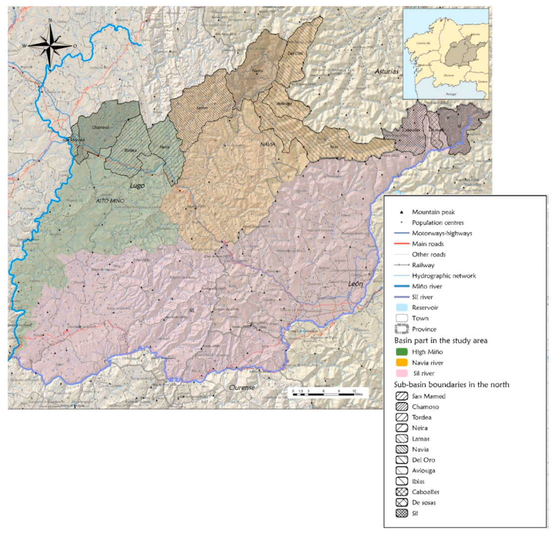
2.1. Study Area
2.2. Fragmentation of the Habitat
2.3. Connectivity
2.3.1. Mapping Data and Data Pre-treatment
2.3.2. Selection of the Reference Species
2.3.3. Choice of Sources
2.3.4. Assigning Impedances (Resistance to Movement)
2.3.5. Distance Cost and Route Cost
2.3.6. Least Cost Paths
2.3.7. Connectivity Indices
3. Results and Discussion
3.1. Fragmentation
3.1.1. Landscape Level
3.1.2. Class Level
3.2. Connectivity
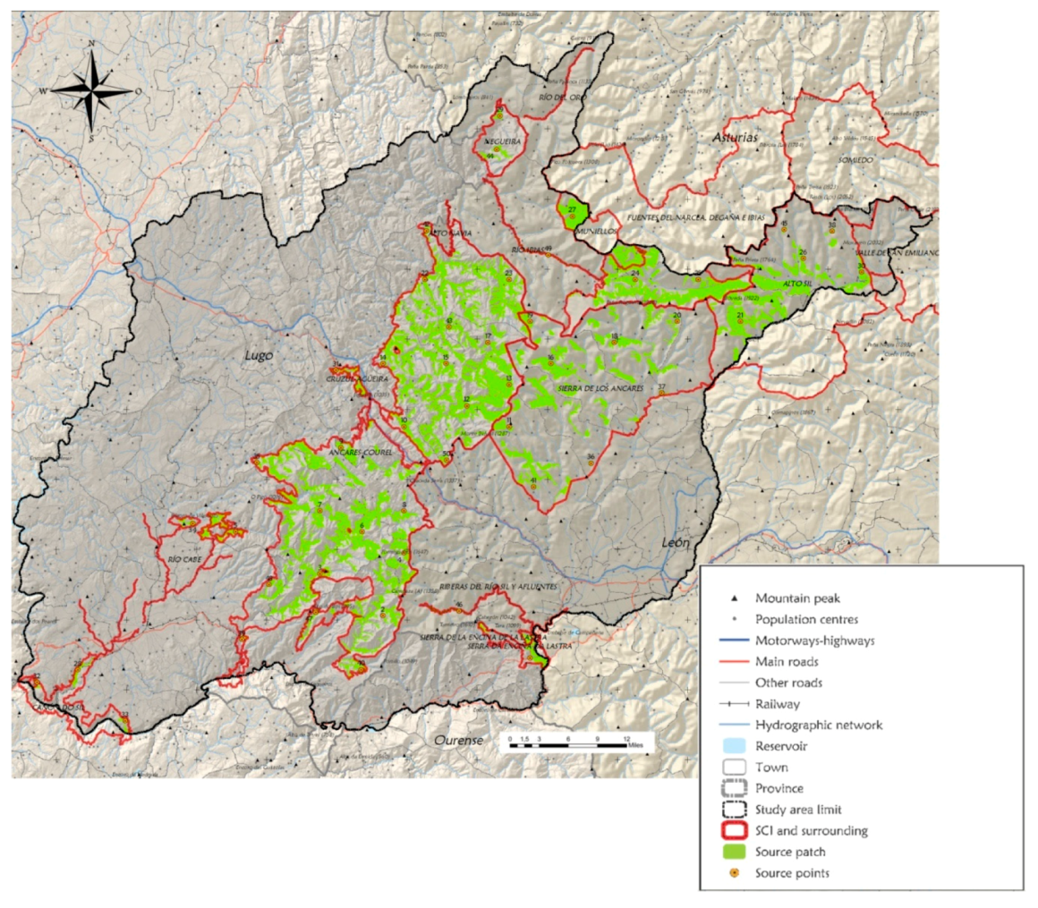
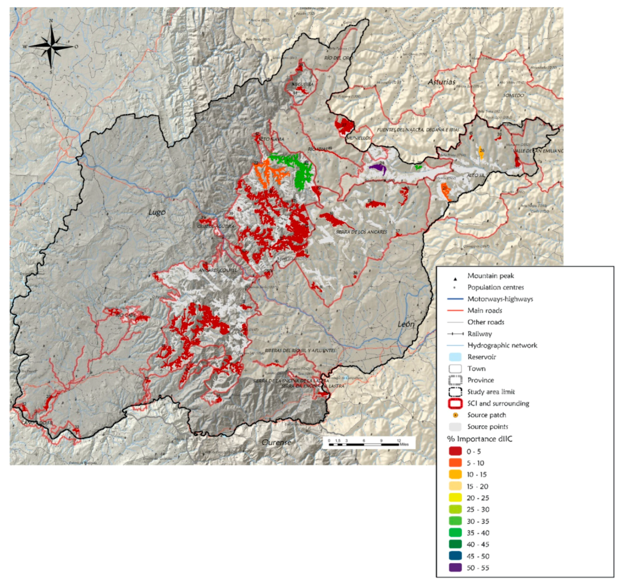
3.2.1. Sources
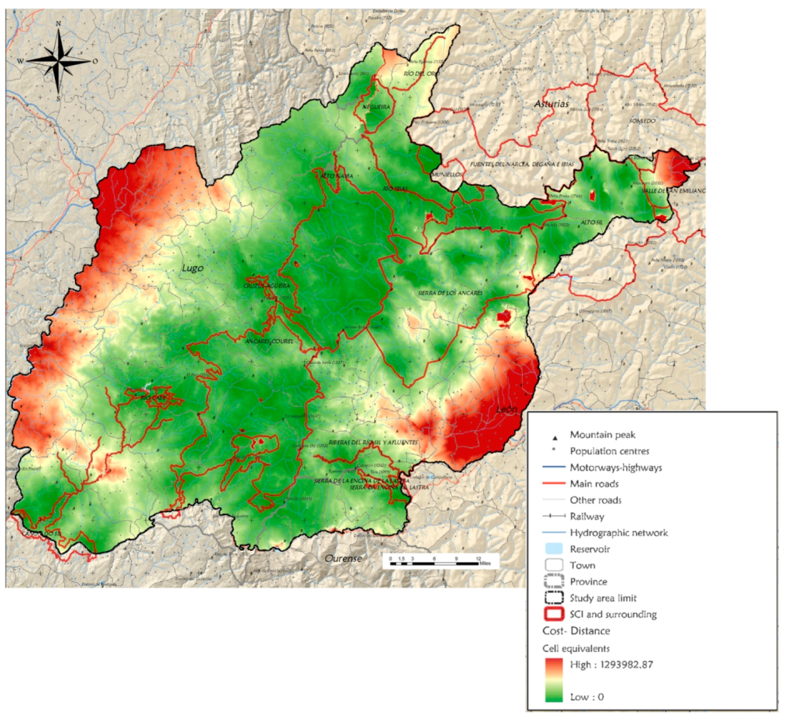
3.2.2. Cost Distances
3.2.3. Effective Distances between Sources
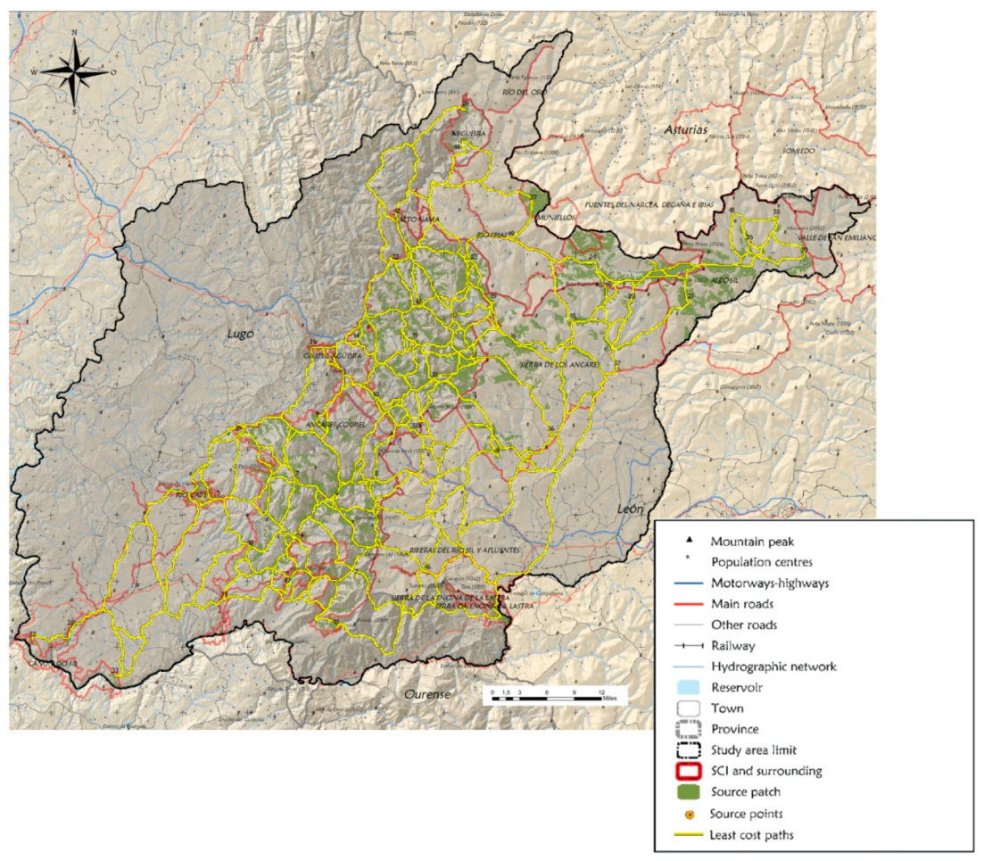
3.2.4. Least Cost Paths
3.2.5. Connectivity for Distinct Dispersal Distances
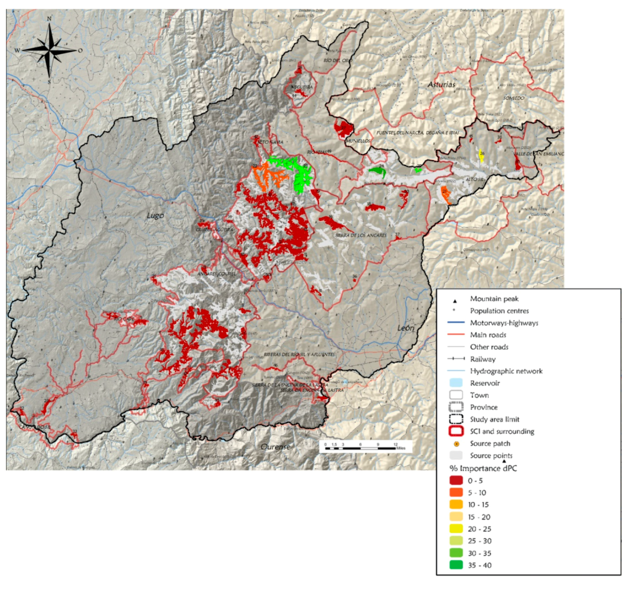
3.2.6. Influence of Connectivity in Decision Making
4. Conclusions
Author Contributions
Funding
Acknowledgments
Conflicts of Interest
Appendix A

| (a) SITEB Classification | Regrouping | Code |
|---|---|---|
| Coastal shoreline lagoons | Sea waters and coastal lagoons | 1 |
| Offshore deep seawaters | ||
| Near shore seawaters | ||
| Large reservoirs | Continental waters | 2 |
| Flowing waters | ||
| Still waters | ||
| Small reservoirs | ||
| Small, seminatural wetlands with heavy use | Wetlands | 3 |
| Pinewoods | Conifers | 4 |
| Forestry plantations of allochthonous Gymnospermae | ||
| Natural conifer woods | ||
| Beaches | Beaches and dunes | 5 |
| Fossilized dune systems | ||
| Active coastal dunes | ||
| Consolidated dunes | ||
| High peat bogs | Peat bogs | 6 |
| Low peat bogs | ||
| Peat bogs with cover | ||
| Waste tips and landfill | ||
| Recreational routes and paths | ||
| Overland communication routes | ||
| Ports, airports and railways (not communication routes) | ||
| Population centres | ||
| Power supply lines | Artificial coverage | 7 |
| Water supply and management infrastructures | ||
| Farm, forestry and fish farming buildings | ||
| Industrial or commercial buildings | ||
| Abandoned buildings, farms and outbuildings | ||
| Mines | ||
| Sports, recreation or non-residential areas | ||
| Temporarily disturbed areas | ||
| Forestry plantations of allochthonous Gymnospermae | Plantations of eucalyptus and other leafy varieties | 8 |
| Eucalyptus woods | ||
| Gallery formation dominated by invasive species | Acacias and other invasive species | 9 |
| Formations of invasive species | ||
| Forestry plantations of autochthonous species | Leafy deciduous trees | 10 |
| Birch woods | ||
| Deciduous oak woods | ||
| Beech woods | ||
| Cork and deciduous oak woods | ||
| Rain forest | ||
| Seminatural sweet chestnut woods | ||
| Large areas of ancient forest | ||
| Large areas with ancient forest complexes | ||
| Ravine woods | ||
| Holm oak woods | Leafy evergreens | 11 |
| Holly woods | ||
| Rocky eulittoral morphologies | Rocky coastal morphologies | 12 |
| Slopes and raised coastal deposits | ||
| Coastal cliffs | ||
| Mountain area rural mosaic | Rural Mosaic of fields surrounded by hedgerows | 13 |
| Small enclosed rural plot mosaic | ||
| Rural mosaic of fields surrounded by tree rows | ||
| Rural mosaic of fields surrounded by bush rows | ||
| Rural mosaic of unaligned fields | Rural mosaic of fields without hedgerows | 14 |
| Rural mosaic of trained vines, crop fields and meadows | ||
| Rural mosaic of vine terraces | ||
| Large-scale continental wet grasslands | Wet grasslands | 15 |
| Medium-scale wet grasslands | ||
| Large areas of irrigated intensive farmland | Large areas of intensive farmland | 16 |
| Large areas of unirrigated farmland | ||
| Scrubland and limestone rocks | Scrubland | 17 |
| Scrubland and mountain rocks | ||
| Scrubland and serpentinic rocks | ||
| Scrubland and siliceous rocks | ||
| Scrubland and ultramafic rocks | ||
| Wet continental scrubland | ||
| Large areas of scrubland with harmless legumes | ||
| Large areas of sub-sclerophyll scrubland | ||
| Large areas of heath | ||
| Wet intradune depressions | Coastal wet area | 18 |
| Estuaries | ||
| Mudflats | ||
| Large areas of shore reed beds |
| (a) Description According to SIOSE | Regrouping | Code |
|---|---|---|
| Crops. Woody crops. Fruit trees. Citrus trees | Crops and Pasture | S01 |
| Crops. Woody crops. Fruit trees. Non-citrus trees | ||
| Crops. Woody crops. Vineyards | ||
| Crops. Woody crops. Olive groves | ||
| Crops. Woody crops. Others | ||
| Crops. Pasture and meadowland | ||
| Pasture | ||
| Crops. Herbaceous crops. Herbaceous crops other than rice | ||
| Crops. Herbaceous crops. Rice | ||
| Forestry woodland. Leafy varieties. Evergreens | Forestry woodland. Leafy varieties. Evergreens | S02 |
| Forestry woodland. Leafy varieties. Deciduous varieties | Forestry woodland. Leafy varieties. Deciduous varieties | S03 |
| Forestry woodland. Conifers | Forestry woodland. Conifers | S04 |
| Scrubland | Scrubland | S05 |
| Land with no vegetation. Boulders. Rocky outcrops and boulders | Land with no vegetation | S06 |
| Land with no vegetation. Bare land | ||
| Land with no vegetation. Burnt areas | ||
| Land with no vegetation. watercourse | ||
| Land with no vegetation. Glaciers and permanent snow | ||
| Land with no vegetation. Boulders. Scree | ||
| Land with no vegetation. Boulders. Quaternary lava outflows | ||
| Artificial cover. Artificial green area and urban treeland | Artificial cover | S07 |
| Artificial cover. Way, parking area or pedestrian area with no vegetation | ||
| Artificial cover. Other buildings | ||
| Artificial cover. Unbuilt-on land | ||
| Artificial cover. Extraction area or tip | ||
| Artificial cover. Building | ||
| Wet cover. Continental wetlands. Marshy areas | Marshy areas | S08 |
| Wet cover. Continental wetlands. Peat bogs | Peat bogs | S09 |
| Artificial cover. Artificial layer of water | Continental waters | S10 |
| Water cover. Continental waters. Water courses | ||
| Water cover. Continental waters. Layers of water. Lakes and Pools. | ||
| Water cover. Continental waters. Layers of water. Reservoirs | ||
| Water cover. Sea waters. Coastal lagoons | Sea waters and coastal lagoons | S11 |
| Water cover. Sea waters. Estuaries | ||
| Water cover. Sea waters. Seas and oceans | ||
| Wet cover. Continental wetlands. Continental salt flats | Salt flats and mud flats | S12 |
| Wet cover. Marine wetlands. Mud flats | ||
| Wet cover. Marine wetlands. Salt flats | ||
| Land with no vegetation. Boulders. Marine cliffs | Marine cliffs | S13 |
| Land with no vegetation. Beaches, dunes and sands | Beaches, dunes and sands | S14 |
| Entry Information | Proportional Scale |
|---|---|
| Land Belonging to Galicia | |
| Information on cover and land uses from SIOSE | 01:25.0 |
| Information on land uses drawn up by SITGA (Sistema de Información Territorial de Galicia) | 01:25.0 |
| Information on communication routes drawn up by SITGA | |
| Motorway and highway | 01:25.0 |
| Provincial roads | 01:25.0 |
| Main and complementary road network | 01:25.0 |
| Trunk roads | 01:25.0 |
| National network | 01:25.0 |
| Secondary network | 01:25.0 |
| Railway | 01:25.0 |
| Hydrographic network | 01:25.0 |
| Natural spaces | |
| SCI | 01:05.0 |
| ZEPVN (Zonas de Especial Protección de los Valores Naturales) | 01:25.0 |
| Digital Land Model (DLM) | 01:25.0 |
| Land Belonging to León And Asturias | |
| Information on cover and land uses from SIOSE | 01:25.0 |
| Digital Land Model (DLM) | 04:20.0 |
| Information on Communication Routes | 04:20.0 |
| Administrative boundaries | 04:20.0 |
| Hydrography | |
| Water basins to one sea | Generated from the 100×100-cell DLM |
| River or riverbed | 04:20.0 |
| Reservoir | 04:20.0 |
| Protected spaces | 04:20.0 |
| Parameter | Acronym | Unit | Calculation Level | |||
|---|---|---|---|---|---|---|
| Total surface area | Area | AREA/CA/TA | ha | P | C | L |
| Patch perimeter | Patch perimeter | PERIM | m | P | ||
| Area | Radius of gyration | GYRATE | m | P | C | L |
| Perimeter-area ratio | Perimeter-area ratio | PARA | - | P | C | L |
| Shape index | Shape index | SHAPE | - | P | C | L |
| Fractal dimension index | Fractal dimension index | FRAC | - | P | C | L |
| Proximity index | Proximity index | PROX | - | P | ||
| Surface proportion of the class | Percentage of landscape | PLAND | % | C | ||
| Number of patches | Number of patches | NP | - | C | L | |
| Patch density | Patch density | DP | patches/km2 | C | L | |
| Patch area mean | Patch area mean | AREA_MN | ha | C | L | |
| Patch area standard deviation | Patch area standard deviation | AREA_SD | ha | C | L | |
| Total edge | Total edge | TE | m | C | L | |
| Edge density | Edge density | ED | m/ha | L | ||
| Area mean | Radius of gyration mean | GYRATE_MN | m | C | L | |
| Perimeter-area ratio mean | Perimeter-area ratio mean | PARA_MN | - | C | L | |
| Shape index mean | Shape index mean | SHAPE_MN | - | C | L | |
| Fractal dimension index mean | Fractal dimension index mean | FRAC_MN | - | C | L | |
| Proximity index mean | Proximity index mean | PROX_MN | - | C | L | |
| Euclidean Nearest Neighbor Distance mean | Euclidean Nearest Neighbour Distance mean | ENN_MN | m | C | L | |
| Interspersion & Juxtaposition Index | Interspersion and juxtaposition index | IJI | % | C | L | |
| Patch Richness (PR) | Patch richness | PR | - | L | ||
| Shannon’s Diversity Index | Shannon’s Diversity Index | SHDI | - | L | ||
| Simpson’s Evenness Index | Simpson’s Evenness Index | SIEI | - | L | ||
References
- Sliva, L.; Williams, D.D. Buffer Zone Versus Whole Catchment Approaches to Studying Land Use Impact on River Water Quality. Water Res. 2001, 35, 3462–3472. [Google Scholar] [CrossRef]
- Li, S.; Gu, S.; Tan, X.; Zhang, Q. Water Quality in the Upper Han River Basin, China: The Impacts of Land Use/Land Cover in Riparian Buffer Zone. J. Hazard. Mater. 2009, 165, 317–324. [Google Scholar] [CrossRef] [PubMed]
- Linneker, B.; Spence, N. Road Transport Infrastructure and Regional Economic Development: The Regional Development Effects of the M25 London Orbital Motorway. J. Transp. Geogr. 1996, 4, 77–92. [Google Scholar] [CrossRef]
- Graham, S. Constructing Premium Network Spaces: Reflections on Infrastructure Networks and Contemporary Urban Development. Int. J. Urban Reg. Res. 2000, 24, 183–200. [Google Scholar] [CrossRef]
- Levin, N.; Watson, J.E.M.; Joseph, L.N.; Grantham, H.S.; Hadar, L.; Apel, N.; Perevolotsky, A.; DeMalach, N.; Possingham, H.P.; Kark, S. A Framework for Systematic Conservation Planning and Management of Mediterranean Landscapes. Biol. Conserv. 2013, 158, 371–383. [Google Scholar] [CrossRef]
- Adeel, Z.; Safriel, U.; Niemeijer, D.; White, R. Ecosystems and Human Well-Being: Desertification Synthesis; Assessment, Millennium Ecosystem; World Resources Institute: Washington, DC, USA, 2005. [Google Scholar]
- Jetz, W.; Wilcove, D.S.; Dobson, A.P. Projected Impacts of Climate and Land-Use Change on the Global Diversity of Birds. PLOS Biol. 2007, 5, e157. [Google Scholar] [CrossRef] [PubMed]
- Natura 2000. European Commission; Natura: Brussels, Belgium, 2009; pp. 1–16. [Google Scholar]
- Council of the European Union. Council Directive 92/43/EEC of 21 May 1992 on the Conservation of Natural Habitats and of Wild Fauna and Flora. Off. J. Eur. Communities 1992, 206, 7–49. [Google Scholar]
- Opermanis, O.; MacSharry, B.; Evans, D.; Sipkova, Z. Is the Connectivity of the Natura 2000 Network Better across Internal or External Administrative Borders? Biol. Conserv. 2013, 166, 170–174. [Google Scholar] [CrossRef]
- Debinski, D.M.; Holt, R.D. A Survey and Overview of Habitat Fragmentation Experiments. Conserv. Biol. 2000, 14, 342–355. [Google Scholar] [CrossRef]
- Crooks, K.R.; Burdett, C.L.; Theobald, D.M.; Rondinini, C.; Boitani, L. Global Patterns of Fragmentation and Connectivity of Mammalian Carnivore Habitat. Philos. Trans. R. Soc. Lond. B Biol. Sci. 2011, 366, 2642–2651. [Google Scholar] [CrossRef]
- Coulon, A.; Cosson, J.F.; Angibault, J.M.; Cargnelutti, B.; Galan, M.; Morellet, N.; Petit, E.; Aulagnier, S.; Hewison, A.J.M. Landscape Connectivity Influences Gene Flow in a Roe Deer Population Inhabiting a Fragmented Landscape: An Individual–Based Approach. Mol. Ecol. 2004, 13, 2841–2850. [Google Scholar] [CrossRef] [PubMed]
- Mazaris, A.D.; Papanikolaou, A.D.; Barbet-Massin, M.; Kallimanis, A.S.; Jiguet, F.; Schmeller, D.S.; Pantis, J.D. Evaluating the Connectivity of a Protected Areas’ Network under the Prism of Global Change: The Efficiency of the European Natura 2000 Network for Four Birds of Prey. PLoS ONE 2013, 8, e59640. [Google Scholar] [CrossRef] [PubMed]
- Sawaya, M.A.; Kalinowski, S.T.; Clevenger, A.P. Genetic Connectivity for Two Bear Species at Wildlife Crossing Structures in Banff National Park. Proc. Biol. Sci. 2014, 281, 20131705. [Google Scholar] [CrossRef] [PubMed]
- Adriaensen, F.; Chardon, J.P.; De Blust, G.; Swinnen, E.; Villalba, S.; Gulinck, H.; Matthysen, E. The application of ‘‘least cost’’ modeling as a functional landscape model. Land. Urban Plan. 2003, 64, 233–247. [Google Scholar] [CrossRef]
- Mallarach, J.M.; Marull, J. Impact assessment of ecological connectivity at the regional level: Recent developments in the Barcelona Metropolitan Area. Impact Assess. Proj. Apprais. 2006, 24, 127–137. [Google Scholar] [CrossRef]
- Cumming, S.G.; Vernier, P. Statistical models of landscape pattern metrics, with applications to regional scale dynamic forest simulations. Land. Ecol. 2002, 17, 433–444. [Google Scholar] [CrossRef]
- Decout, S.; Manel, S.; Miaud, C.; Luque, S. Integrative approach for landscape-based graph connectivity analysis: A case study with the common frog (Rana temporaria) in humandominated Landscapes. Landsc. Ecol. 2012, 27, 267–279. [Google Scholar] [CrossRef]
- Carballeira, A.; Devesa, C.; Retuerto, R.; Santillan, E.; Fernando, U. Bioclimatología de Galicia; Fundación Pedro Barrié de la Maza: Coruña, Spain, 1983. [Google Scholar]
- Martínez Cortizas, A.; Pérez Alberti, A. Atlas Climático de Galicia; Xunta de Galicia, Consellería de Medio Ambiente: Santiago de Compostela, Spain, 2000. [Google Scholar]
- Xunta de Galicia. Sistema de Información Territorial y de la Biodiversidad de Galicia. Available online: http://inspire.xunta.es/website/SITEB2/viewer.htm (accessed on 25 October 2016).
- McGarigal, K.; Cushman, S.; Neel, M.; Ene, E. FRAGSTATS: Spatial Pattern Analysis Program for Categorical Maps. Computer Software Program; University of Massachusetts: Amherst, MA, USA, 2002. [Google Scholar]
- Freemark, K.; Bert, D.; Villard, M.-A. Patch-, Landscape-, and Regional-Scale Effects on Biota. In Applying Landscape Ecology in Biological Conservation; Gutzwiller, K.J., Ed.; Springer: New York, NY, USA, 2002; pp. 58–83. [Google Scholar] [CrossRef]
- Xunta de Galicia. Sistema de InformaciónsobreOcupación del Suelo de España. Available online: http://www.siose.es/siose/index.html (accessed on 25 June 2016).
- Xunta de Galicia. Sistema de Información Territorial de Galicia. Available online: http://mapas.xunta.gal/portada (accessed on 10 June 2016).
- Clevenger, A.; Purroy, F.J.; Pelton, M.R. Brown Bear (Ursus Arctos L.) Habitat Use in the Cantabrian Mountains, Spain. Mammalia 1992, 56. [Google Scholar] [CrossRef]
- Ley 42/2007, de 13 de Diciembre, del Patrimonio Natural y de La Biodiversidad. Available online: https://www.boe.es/buscar/pdf/2007/BOE-A-2007-21490-consolidado.pdf (accessed on 31 May 2016).
- Real Decreto 139/2011, de 4 de Febrero, Para El Desarrollo Del Listado de EspeciesSilvestresEnRégimen de Protección Especial y Del CatálogoEspañol de EspeciesAmenazadas. Available online: https://www.boe.es/buscar/pdf/2011/BOE-A-2011-3582-consolidado.pdf (accessed on 31 May 2016).
- De Galicia, X. Decreto 88/2007 Do 19 de Abril, Polo Que Se Regula o Catálogo Galego de EspeciesAmeazadas. D. Oficial de Galicia 2007, 89, 7409–7423. [Google Scholar]
- Zeller, K.A.; McGarigal, K.; Whiteley, A.R. Estimating Landscape Resistance to Movement: A Review. Landsc. Ecol. 2012, 27, 777–797. [Google Scholar] [CrossRef]
- Fahrig, L.; Pedlar, J.H.; Pope, S.E.; Taylor, P.D.; Wegner, J.F. Effect of Road Traffic on Amphibian Density. Biol. Conserv. 1995, 73, 177–182. [Google Scholar] [CrossRef]
- Instituto Nacional de Estadística (INE). Censo Nacional de Población y Vivienda 2001. Available online: http://www.ine.es/censo2001/ (accessed on 31 May 2016).
- Ferreras, P. Landscape Structure and Asymmetrical Inter-Patch Connectivity in a Metapopulation of the Endangered Iberian Lynx. Biol. Conserv. 2001, 100, 125–136. [Google Scholar] [CrossRef]
- Saura, S.; Pascual-Hortal, L. Conefor sensinode 2.2 user’s manual: Software for quantifying the importance of habitat patches for maintaining landscape connectivity through graphs and habitat availability indices. Available online: http://www.conefor.org/files/usuarios/CS22manual.pdf (accessed on 31 May 2016).
- Ray, N. Pathmatrix: A Geographical Information System Tool to Compute Effective Distances among Samples. Mol. Ecol. Notes 2005, 5, 177–180. [Google Scholar] [CrossRef]
- Pascual-Hortal, L.; Saura, S. Comparison and development of new graph-based landscape connectivity indices: Towards the priorization of habitat patches and corridors for conservation. Landsc. Ecol. 2006, 21, 959–967. [Google Scholar] [CrossRef]
- Saura, S.; Rubio, L. A Common Currency for the Different Ways in Which Patches and Links Can Contribute to Habitat Availability and Connectivity in the Landscape. Ecography (Cop.) 2010, 33, 523–537. [Google Scholar] [CrossRef]
- Saura, S.; Appendix, A. Evaluating Forest Landscape Connectivity through ConeforSensinode 2.2. In Patterns and Processes in Forest Landscapes; Springer: Berlin, Germany, 2008; pp. 403–422. [Google Scholar]
- Echeverry, D.M.A.; Rodriguez, P.J.M. Análisis de un paisaje fragmentado como herramienta para la conservación de la biodiversidadenáreas de bosqueseco y subhumedo tropical en el municipio de Pereira, Risaralda Colombia. Sci. Tech. 2006, XII, 405–410. [Google Scholar]
- Mateo-Sánchez, M.C.; Cushman, S.A.; Saura, S. Connecting Endangered Brown Bear Subpopulations in the Cantabrian Range (North-Western Spain). Anim. Conserv. 2014, 17, 430–440. [Google Scholar] [CrossRef]
- Stevens, K.P.; Holland, G.J.; Clarke, R.H.; Cooke, R.; Bennett, A.F. What Determines Habitat Quality for a Declining Woodland Bird in a Fragmented Environment: The Grey-Crowned Babbler Pomatostomus Temporalis in South-Eastern Australia? PLoS ONE 2015, 10, e0130738. [Google Scholar] [CrossRef] [PubMed]
- Smith, T.M.; Smith, R.L. Ecología; Addison Wesley: Madrid, Spain, 2002. [Google Scholar]
- Gurrutxaga, M. Conectividad Ecológica Del Territorio y Conservación de La Biodiversidad. Nuevas Perspectivas EnEcología Del Paisaje y Ordenación Territorial. Available online: https://www.researchgate.net/publication/302252844_Conectividad_ecologica_del_territorio_y_conservacion_de_la_biodiversidad_Nuevas_perspectivas_en_ecologia_del_paisaje_y_ordenacion_territorial (accessed on 31 May 2016).
- Larkin, J.L.; Maehr, D.S.; Hoctor, T.S.; Orlando, M.A.; Whitney, K. Landscape Linkages and Conservation Planning for the Black Bear in West-Central Florida. Anim. Conserv. 2004, 7, 23–34. [Google Scholar] [CrossRef]
- Saura, S.; Torne, J. Conefor Sensinode 2.2: A Software Package for Quantifying the Importance of Habitat Patches for Landscape Connectivity. Environ. Model. Softw. 2009, 24, 135–139. [Google Scholar] [CrossRef]
- Grilo, C.; Sousa, J.; Ascensão, F.; Matos, H.; Leitão, I.; Pinheiro, P.; Costa, M.; Bernardo, J.; Reto, D.; Lourenço, R.; et al. Individual Spatial Responses towards Roads: Implications for Mortality Risk. PLoS ONE 2012, 7, e43811. [Google Scholar] [CrossRef] [PubMed]
- Clevenger, A.P.; Purroy, F.J.; Campos, M.A. Habitat Assessment of a Relict Brown Bear Ursus Arctos Population in Northern Spain. Biol. Conserv. 1997, 80, 17–22. [Google Scholar] [CrossRef]
- Naves, J.; Wiegand, T.; Revilla, E.; Delibes, M. Endangered Species Constrained by Natural and Human Factors: The Case of Brown Bears in Northern Spain. Conserv. Biol. 2003, 17, 1276–1289. [Google Scholar] [CrossRef]
- Mateo Sánchez, M.C.; Cushman, S.A.; Saura, S. Scale Dependence in Habitat Selection: The Case of the Endangered Brown Bear (Ursus Arctos) in the Cantabrian Range (NW Spain). Int. J. Geogr. Inf. Sci. 2014, 28, 1531–1546. [Google Scholar] [CrossRef]
- Gurrutxaga, M. Red de Corredores Ecológicos de la Comunidad Autónoma de Euskadi; IKT para Dept. de Medio Ambiente y Ordenación del Territorio: Gobierno Vasco, Spain, 2005. [Google Scholar]


| (a) Land Use | Code | Impedance | ||
|---|---|---|---|---|
| Crops and meadows | S1 | 30 | ||
| Forest woodland. Leafy evergreen varieties | S2 | 1 | ||
| Forest woodland. Leafy deciduous varieties | S3 | 1 | ||
| Forest woodland-conifers | S4 | 10 | ||
| Scrubland | S5 | 10 | ||
| Land with no vegetation | S6 | 40 | ||
| Artificial covers | S7 | 100 | ||
| Marshylands | S8 | 5 | ||
| Beat bogs | S9 | 5 | ||
| Continental waters | S10 | 70 | ||
| (b) Distance to the Route | Impedance Increment Factor | |||
| Motorways–Highways | Main Roads | Other | Railway | |
| Roads | ||||
| 25 | 1.40 | 1.32 | 1.2 | 1.32 |
| 50 | 1.36 | 1.24 | 1.1 | 1.24 |
| 75 | 1.32 | 1.16 | 1.16 | |
| 100 | 1.28 | 1.08 | 1.08 | |
| 125 | 1.24 | |||
| 150 | 1.20 | |||
| 175 | 1.16 | |||
| 200 | 1.12 | |||
| 225 | 1.08 | |||
| 250 | 1.04 | |||
| Parameter | Acronym | Ancares–Courel SCIs and Their Surroundings |
|---|---|---|
| Area (ha) | TA | 108,420.42 |
| Number of patches | NP | 7417.00 |
| Patch density per km2 | PD | 6.84 |
| Proximity index | PROX_MN | 3756.92 |
| Nearest neighbour distance mean | ENN_MN | 113.08 |
| Juxtaposition index | IJI | 55.65 |
| Patch richness | PR | 11.00 |
| Shannon’s Diversity Index | SHDI | 1.38 |
| Space | Land Use | CA (ha) | PLAND (%) | NP | AREA_MN (ha) | GYRA_MN | SHAPE_MN | FRAC_MN | PROX_MN | IJI |
|---|---|---|---|---|---|---|---|---|---|---|
| Ancares–Courel | Leafy deciduous | 25957.81 | 23.94 | 2673 | 9.71 | 81.68 | 2.01 | 1.12 | 4129.64 | 56.30 |
| Surroundings | Conifers | 7124.16 | 6.57 | 314 | 22.69 | 166.85 | 2.06 | 1.12 | 1324.76 | 53.13 |
| Eucalyptus and other leafy plantations | 2.79 | 0.00 | 3 | 0.93 | 42.38 | 1.45 | 1.09 | 0.00 | 55.96 | |
| Acacias and other invasive species | 13.84 | 0.01 | 5 | 2.77 | 90.78 | 2.12 | 1.14 | 26.36 | 53.83 | |
| Rural mosaic of fields surrounded by hedgerows | 18436.21 | 17.00 | 2347 | 7.86 | 96.95 | 2.16 | 1.14 | 1035.20 | 56.94 | |
| Rural mosaic of fields without hedgerows | 1199.65 | 1.11 | 164 | 7.31 | 113.14 | 1.85 | 1.11 | 67.22 | 58.34 | |
| Scrubland | 51961.15 | 47.93 | 1081 | 48.07 | 191.55 | 2.37 | 1.13 | 12824.18 | 60.11 | |
| Peat bogs | 77.16 | 0.07 | 44 | 1.75 | 57.80 | 2.04 | 1.14 | 6.08 | 61.01 | |
| Leafy evergreens | 418.78 | 0.39 | 44 | 9.52 | 135.41 | 1.99 | 1.12 | 39.91 | 62.58 | |
| Artificial cover | 1109.36 | 1.02 | 574 | 1.93 | 54.82 | 1.56 | 1.09 | 33.63 | 48.37 | |
| Continental waters | 2119.51 | 1.95 | 168 | 12.62 | 450.09 | 8.98 | 1.29 | 508.97 | 51.18 |
| Origin Space | Number Paths that Leave the SCI | Average Value (km) | Minimum Value (km) | Maximum Value (km) |
|---|---|---|---|---|
| Alto Sil | 90 | 2498.62 | 334.38 | 5404.21 |
| Ancares–Courel | 641 | 1445.04 | 99.51 | 3699.56 |
| Sil Canyon | 57 | 3027.02 | 309.89 | 5395.85 |
| Cruzul-Agüeira | 19 | 1482.87 | 553.51 | 2838.01 |
| Fuentes del Narcea, Degaña E Ibias | 51 | 1852.29 | 214.82 | 4339.63 |
| Muniellos | 23 | 1966.34 | 286.04 | 4064.79 |
| Negueira | 27 | 2386.44 | 891.39 | 4411.72 |
| Banks of the river Sil and tributaries | 4 | 1400.54 | 872.58 | 2177.99 |
| River Cabe | 62 | 1775.87 | 210.37 | 3683.38 |
| Serra da Enciña da Lastra | 49 | 2294.5 | 678.49 | 4116.23 |
| Sierra de los Ancares | 202 | 1672.39 | 144.02 | 4451.08 |
© 2019 by the authors. Licensee MDPI, Basel, Switzerland. This article is an open access article distributed under the terms and conditions of the Creative Commons Attribution (CC BY) license (http://creativecommons.org/licenses/by/4.0/).
Share and Cite
Valero, E.; Álvarez, X.; Picos, J. Connectivity Study in Northwest Spain: Barriers, Impedances, and Corridors. Sustainability 2019, 11, 5124. https://doi.org/10.3390/su11185124
Valero E, Álvarez X, Picos J. Connectivity Study in Northwest Spain: Barriers, Impedances, and Corridors. Sustainability. 2019; 11(18):5124. https://doi.org/10.3390/su11185124
Chicago/Turabian StyleValero, Enrique, Xana Álvarez, and Juan Picos. 2019. "Connectivity Study in Northwest Spain: Barriers, Impedances, and Corridors" Sustainability 11, no. 18: 5124. https://doi.org/10.3390/su11185124
APA StyleValero, E., Álvarez, X., & Picos, J. (2019). Connectivity Study in Northwest Spain: Barriers, Impedances, and Corridors. Sustainability, 11(18), 5124. https://doi.org/10.3390/su11185124