Nonlinear Predictive Control for a Boiler–Turbine Unit Based on a Local Model Network and Immune Genetic Algorithm

Abstract

This paper proposes a nonlinear model predictive control (NMPC) strategy based on a local model network (LMN) and a heuristic optimization method to solve the control problem for a nonlinear boiler–turbine unit. First, the LMN model of the boiler–turbine unit is identified by using a data-driven modeling method and converted into a time-varying global predictor. Then, the nonlinear constrained optimization problem for the predictive control is solved online by a specially designed immune genetic algorithm (IGA), which calculates the optimal control law at each sampling instant. By introducing an adaptive terminal cost in the objective function and utilizing local fictitious controllers to improve the initial population of IGA, the proposed NMPC can guarantee the system stability while the computational complexity is reduced since a shorter prediction horizon can be adopted. The effectiveness of the proposed NMPC is validated by simulations on a 500 MW coal-fired boiler–turbine unit.

1. Introduction

During the past 30 years, the technology of renewable energy power generation has been developed rapidly in China. However, the intermittent nature of renewable power sources brings large power fluctuations in electrical power systems, which in turn limits the scale of new energy sources connected into the power grid [1,2].

Coordinated control system (CCS) is used to adjust the power output for grid balance while maintaining other variables, such as main steam temperature, within their safe and economical ranges [2,3]. The ever-increasing load demand requirements bring tough challenges to the CCS of nonlinear boiler–turbine (B-T) units. Proportional integral derivative (PID) and proportional integral (PI) controllers are still widely adopted in the control of thermal power plants due to the ease of use. However, they are only adequate for the regulation of small load variations and cannot meet the requirement of wide-range load operation [4]. Various attempts were carried out to improve the performance of these conventional linear controllers. For instance, a genetic algorithm (GA) was used in our previous research [5] to find the suitable parameters of PI controller and linear quadratic regulator (LQR) for a wide operation of a B-T system. An iterative feedback tuning (IFT) technique [6] and a hybrid jump particle swarm optimization (PSO) [7] were also used to simplify the parameter tuning of PID controllers of the B-T unit. However, these improved PID controllers cannot produce satisfactory performances in case of rapidly-changing operating conditions and, furthermore, have no ability to deal with the operating constraints.

Since model predictive control (MPC) methods are able to explicitly handle the multivariable constrained problem, it became popular in B-T unit control [8,9,10,11,12,13,14,15,16,17,18,19,20,21]. Besides, the dynamic matrix control (DMC) based on the step-response model (SRM) was investigated [8], showing that the SRM based on test data is more suitable than the linearized model because of the severe nonlinearity of drum water-level dynamics. Furthermore, we proposed later in [9] an adaptive dynamic matrix control (DMC) based on an online-interpolated SRM with fuzzy inference to improve the control performance for a wide-range operation. Because of the limitation of linear controllers in dealing with nonlinear problems [10], neural networks [11,12] and neuro-fuzzy network [13] were designed for the B-T unit. A superior wide-range load variation can be achieved by these nonlinear MPCs (NMPCs), while they have heavy computational burden and their models lack explicit physical significance, which may lead to difficulty in dynamic analysis and model transparency.

An explicit MPC based on a piecewise affine model was developed in [14], and simulation results show that its robustness against output noise is superior to H1 control and the control efforts are smaller. Wang et al. [15] developed a double-layered multi-model predictive control based on piecewise step-response models for an ultra-supercritical power unit. The fuzzy modeling technique has also been integrated with MPC for the B-T unit [16,17,18,19,20,21]. Based on the fuzzy model, an offset-free MPC using a genetic algorithm [16] and a nonlinear model predictive iterative learning control [17] were presented for a 160 MW drum-type B-T unit, which were shown to be effective in a wide-range operation. Subspace identification (SID) and fuzzy clustering methods were used by Wu and others to design the data-driven MPCs for the B-T system [18,19,20,21]. These data-driven control methods are flexible and can be adapted to the system without knowing mathematical models of the plant, whereas they are excessively dependent on the sampled data and have no clearly defined structure.

In recent years, much attention has also been paid to the improvement of the robustness against unknown uncertainties and external disturbances for the B-T unit control, such as L1 adaptive state feedback control [22], sliding mode control [23,24,25], adaptive variable structure, and H∞ robust optimal control [26]. The idea of improving robustness of energy systems is further explored by active disturbance rejection control (ADRC) approaches [27,28], such as nonlinear disturbance rejection control with the combination of a stable feedback controller and a sliding mode observer [29], ADRC based on direct energy balance [30], and robust mode predictive control [31,32]. However, most of these approaches, except two enhanced MPCs in [31] and [32], cannot effectively deal with the constraints, which may deteriorate the control performance of CCS in practice. Moreover, except for [30], the models, on which these control strategies are based, are derived from the provided nonlinear mathematical model, which is actually not easily obtained for real power plants.

Various advanced control strategies used in the B-T unit control have shown their superiority in some respects. However, there are still some shortcomings in these approaches, such as in terms of constraint handling, model acquisition, or computational complexity. Multi-model predictive control (MMPC) is more flexible and easier to implement than other nonlinear control approaches, and superior performance can be attained. However, the nonlinear variation of prediction model in prediction horizon is rarely considered in many existing MMPCs, especially when the prediction model is obtained by linearization. In general, it is assumed that the system’s behavior is constant or changes slowly in the whole prediction horizon, and the fixed model in the current instant is used to forecast system outputs; therefore, the stability of the control system can only rely on the limited robustness of the MPC. Obviously, the stability of these MMPCs cannot be guaranteed when the B-T units have to change load quickly in a wide range. Therefore, a new nonlinear predictive control based on a multi-model framework will be proposed in this paper to effectively solve the B-T unit control problem.

The advantage of the model-weighted MMPC is that the chattering problem caused by the scheduling of multiple local controllers can be avoided. Moreover, the controller can make full use of all dynamic information of the system at each sampling instant and comprehensively optimize control variables, so that better global control performance can be obtained. For these reasons, in this paper we will design an improved model-weighted MMPC for a B-T unit, that is, a nonlinear predictive control approach based on a local model network (LMN) and optimized by a heuristic optimization method (i.e., an immune genetic algorithm (IGA)). The proposed control strategy has the following contributions and advantages:

(1) The modeling problem of the nonlinear B-T unit in a wide-range operation is solved by using a data-driven iterative identification method to develop an accurate LMN model.

(2) A special IGA is designed to solve the nonlinear constrained optimization problem for the predictive control based on the LMN model.

(3) The terminal cost with an adaptively-switched weight matrix is introduced into the objective function of NMPC and local fictitious controllers are utilized to accelerate IGA, thus the stability of the system can be implicitly guaranteed and online computational burden is decreased.

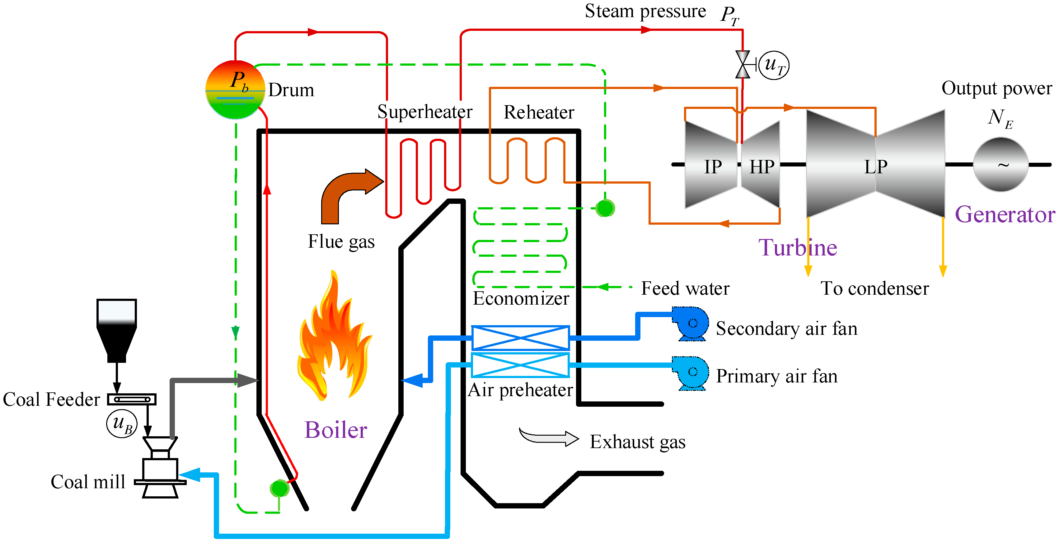
2. System Description

A schematic of a typical coal-fired subcritical drum-type boiler–turbine unit is shown in Figure 1. The boiler transfers the chemical energy of fuel into the thermal energy of steam, which is directly fed to the turbine where the thermal energy is converted into mechanical energy and the generator is driven to generate electricity. The B-T unit can be regarded as a nonlinear multivariable system with two inputs and two outputs. The outputs or the controlled variables are the power output, $N_E$ (MW) and the main steam pressure, $P_T$ (MPa). The inputs or manipulated variables are the normalized fuel feed $u_B$ and the turbine control valve position $u_T$. The control objective of the CCS is to achieve fast power tracking while maintaining the main steam pressure within an acceptable range [30] (in constant-steam-pressure mode) or keeping the main steam pressure accurately following its set-point (in variable-steam-pressure mode).

A nonlinear dynamic model representing a 500 MW subcritical B-T unit in Shentou #2 power plant in Shanxi Province, China [33], is used as the controlled object in this paper. The model accuracy was verified by the field data. The model is in the form of

$$\{\begin{array}{l}{\dot{x}}_1=0.8673{\left(x_2-x_1\right)}^{\frac{1}{2}}-0.0895x_1{u}_2\\ {\dot{x}}_2=-0.0964{\left(x_2-x_1\right)}^{\frac{1}{2}}+0.1616x_4\\ {\dot{x}}_3=\left(-x_3+u_1\right)/98\\ {\dot{x}}_4=\left(-x_4+x_3\right)/6\\ {\dot{x}}_5=-x_5+0.303\times 101.9778x_1{u}_2\\ y_1=x_5\\ y_2=x_1\end{array}$$

(1)

where $x_1\left(y_2\right)$ is main steam pressure $P_T$ (MPa); $x_2$ is drum pressure $P_b$ (MPa); $x_3$ is the normalized boiler combustion intensity; $x_4$ is the normalized effective heat absorption of the boiler; and $x_5\left(y_1\right)$ is output power $N_E$ (MW). The two manipulated variables $u_1\left(u_B\right)$ and $u_2\left(u_T\right)$ are subject to the actuator constraints:

$$\left|u_1\right|\le 100\%, \left|u_2\right|\le 100\%, \left|{\dot{u}}_1\right|\le 5\%, \left|{\dot{u}}_2\right|\le 10\%$$

(2)

To achieve the control objective of CCS, a novel NMPC strategy based on LMN and IGA is proposed for the B-T unit as shown in Figure 2, where $\mathit{u}\left(k\right)$ and $\mathit{y}\left(k\right)$ are, respectively, the control inputs and the outputs of the B-T unit, $\mathit{u}\left(k+j|k\right)\left(j=0,1,\dots ,N_t-1\right)$ are the predictive control sequence given by the NMPC, and $\widehat{\mathit{y}}\left(k+j|k\right)\left(j=0,1,\dots ,N_t-1\right)$ are the predictive outputs of the LMN. The LMN model obtained by off-line identification based on input-output data can be used to predict the process outputs, and then a dynamic optimization problem will be formulated to determine the optimal control inputs. Due to the constraint conditions and the nonlinearity of the prediction model, a heuristic optimization technique (i.e., IGA) is used for iterative optimization. The IGA solves the optimization problem at every sampling period to find the optimal control sequence that can meet the constraints and minimize the objective function (performance index).

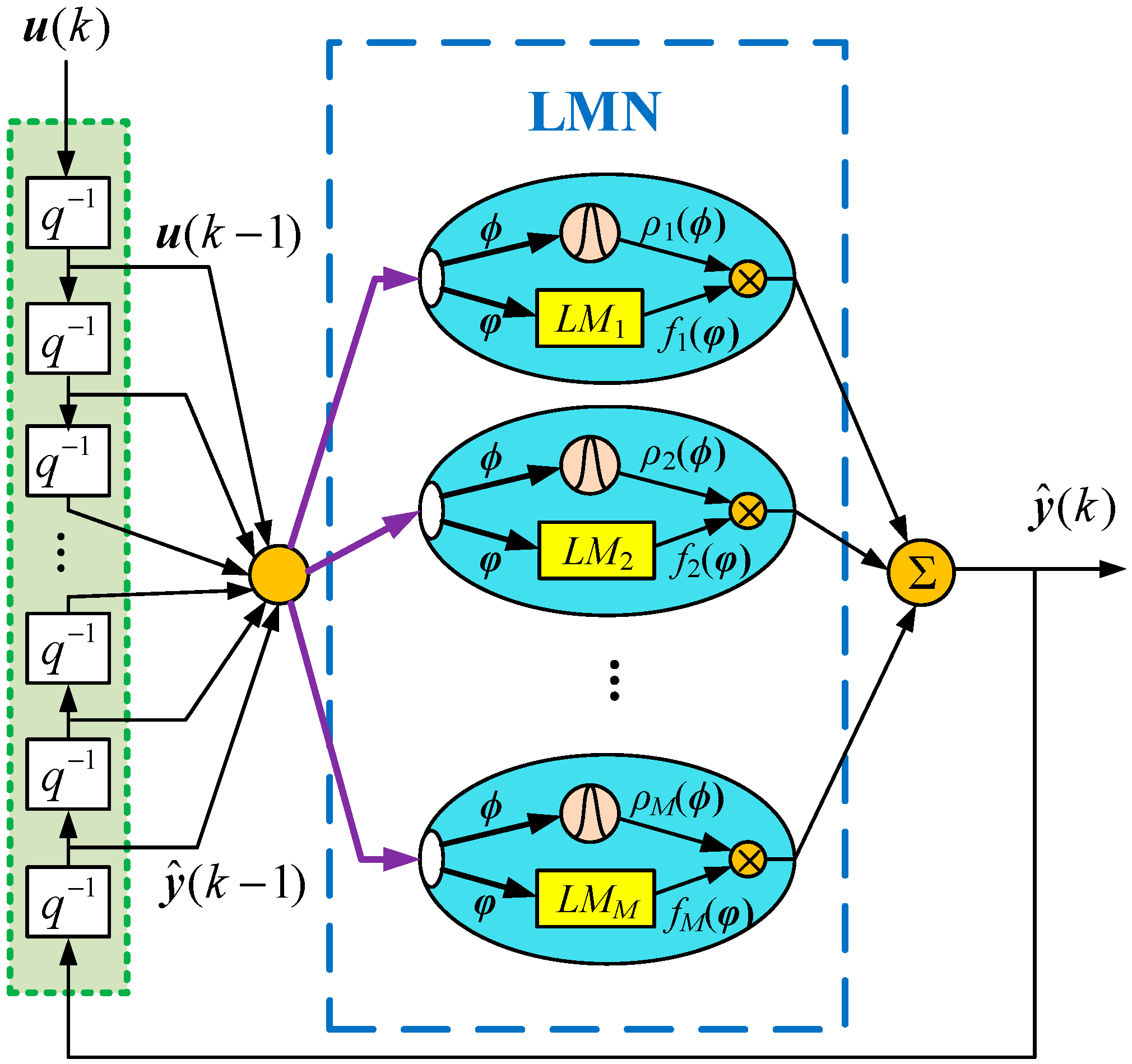
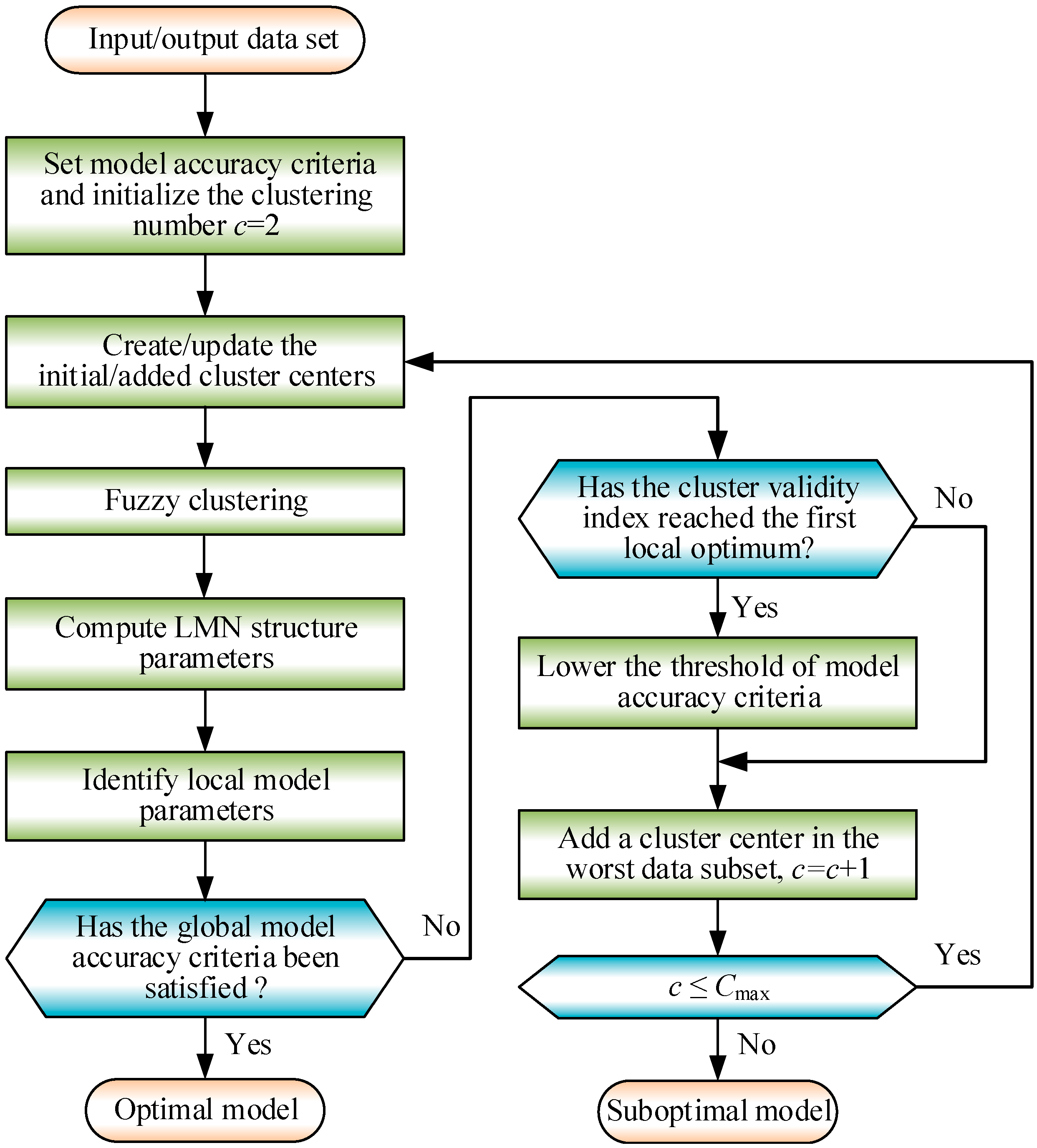
3. Data-Driven Modeling of the B-T Unit

The dynamic characteristics of the B-T unit in different operating conditions are reflected in the operation data. Therefore, we can make full use of these operation data and adopt a data-driven modeling strategy to obtain the model of the process for the controller design.

Conventional neural networks and fuzzy logic-based models are usually of high computational cost and have the potential of overfitting. As an alternative multi-model approach, a local model network (LMN) [34] is adopted in this paper. Besides interpretability, in comparison to the widely-used radial basis function network (RBFN) model, each local model in the LMN can cover a larger subspace than each neuron in RBFN, meaning that the number of local models needed can be substantially reduced [35].

Figure 3 depicts the structure of a dynamic LMN, where each local model consists of two parts [36]: the dynamic model $f_i(\cdot )$ and its validity function ${\rho }_i(\cdot )$. For a multivariable system with R inputs and S outputs, the LMN can be represented as follows:

$$\mathit{y}\left(k\right)={\displaystyle \sum _{i=1}^M{\rho }_i\left(\mathit{\varphi }\left(k\right)\right)\cdot f_i\left(\mathit{\varphi }\left(k\right)\right)}$$

(3)

where M is the number of local models; $f_i(\cdot )$ $\left(i=1,\dots ,M\right)$ are local models defined as functions of current r-dimensional measurement vector or scheduling vector $\mathit{\phi }\left(k\right)\in R^r$, which defines the operating point of the system; and ${\rho }_i(\cdot )$ are respective local model validity functions defined as functions of current L-dimensional operating region vector $\mathit{\varphi }\left(k\right)\in R^L$, which contains past system inputs and outputs.

A commonly-chosen validity function in LMN is the normalized Gaussian function defined as:

$${\rho }_i\left(\mathit{\varphi }\right)=\frac{{\beta }_i\left(\mathit{\varphi }\right)}{{\displaystyle \sum _{i=1}^M{\beta }_i\left(\mathit{\varphi }\right)}}, {\beta }_i\left(\mathit{\varphi }\right)=\exp \left[-\frac{{\left(\mathit{\varphi }-{\mathit{c}}_i\right)}^T\left(\mathit{\varphi }-{\mathit{c}}_i\right)}{{\sigma }_i^2}\right]$$

(4)

where ${\mathit{c}}_i$ and ${\sigma }_i$ are the center and width of the Gaussian interpolation functions, respectively. The valid domain of the i-th local model can be described as ${\mathit{\Gamma }}_i\in \left[{\mathit{c}}_i-{\sigma }_i{\mathit{I}}_e,{\mathit{c}}_i+{\sigma }_i{\mathit{I}}_e\right]$, in which ${\mathit{I}}_e={\left[1,1,\dots ,1\right]}^T\in R^r$.

Assume that the controlled auto-regressive moving average (CARMA) models are chosen as the representation of linear local models:

$${\mathit{A}}_i\left(q^{-1}\right)\mathit{y}\left(k\right)={\mathit{B}}_i\left(q^{-1}\right)\mathit{u}\left(k-1\right)$$

(5)

where ${\mathit{A}}_i$ and ${\mathit{B}}_i$ are the polynomials in the backward shift operator $q^{-1}$, ${\mathit{A}}_i\left(q^{-1}\right)=\mathit{I}+{\mathit{A}}_{i1}{q}^{-1}+\cdots +{\mathit{A}}_{i{n}_A}{q}^{-n_A}$ and ${\mathit{B}}_i\left(q^{-1}\right)={\mathit{B}}_{i0}+{\mathit{B}}_{i1}{q}^{-1}+\cdots +{\mathit{B}}_{i{n}_B}{q}^{-n_B}$; ${\mathit{A}}_{ij}\in R^{S\times S},j=1,\dots ,n_A$; ${\mathit{B}}_{ij}\in R^{S\times R},j=0,\dots ,n_B$; $n_A$ is the number of delayed input samples and $n_B$ is the number of delayed output samples.

Define the regression vector ${\mathit{\phi }}^T\left(k\right)={\left[-{\mathit{y}}^T\left(k-1\right),\dots ,-{\mathit{y}}^T\left(k-n_A\right),{\mathit{u}}^T\left(k-1\right),\dots ,{\mathit{u}}^T\left(k-n_B-1\right)\right]}^T$ and the parameter vector ${\mathit{\theta }}_i={\left[{\mathit{A}}_{i1},\dots ,{\mathit{A}}_{i{n}_A},{\mathit{B}}_{i0},\dots ,{\mathit{B}}_{i{n}_B}\right]}^T$, then the local model (5) can be expressed in a regression form:

$${\mathit{y}}_i^T\left(k\right)=f_i\left(\mathit{\phi }\left(k\right)\right)={\mathit{\phi }}^T\left(k\right){\mathit{\theta }}_i,i=1,2,\dots ,M$$

(6)

Substituting (6) into (3), we have the global model which is a combination of local models,

$${\mathit{y}}^T\left(k\right)={\displaystyle \sum _{i=1}^M{\rho }_i\left(\mathit{\varphi }\left(k\right)\right)}{\mathit{\phi }}^T\left(k\right){\mathit{\theta }}_i$$

(7)

The identification of LMN includes choosing a suitable scheduling variable $\mathit{\varphi }$ and determining the number of local models M as well as the validity functions ${\rho }_i(\cdot )$ and parameter vector ${\mathit{\theta }}_i$. With an incorporation of prior knowledge, some expected behaviors of the system can help simplify the identification procedure of LMN [37]. However, the worst case is considered in this paper (i.e., assuming that we have no prior knowledge), and only historical operation data can be utilized to obtain the model of the B-T unit.

A data-driven multi-model modeling method on the basis of the satisfactory fuzzy clustering technique was proposed by Zhu, Shen and Li [38], where the identification procedure is as shown in Figure 4. The data set composed of the scheduling vector and output of the system $\left\{z_k={\left[{\mathit{\varphi }}^T\left(k\right),\mathit{y}\left(k\right)\right]}^T,k=1,2,\dots ,N\right\}$ is used for clustering. The structure of the LMN is determined directly from the clustering result (i.e., the number of local models is equal to the number of clustering centers) and at the same time the parameters $\left({\mathit{c}}_i,{\sigma }_i\right)$ of the validity function ${\rho }_i(\cdot )$ are determined according to the position of the clustering centers. Since the clustering number c is chosen based on the combination of model accuracy requirement and cluster validity index, redundant local models can be avoided. The parameters of the local models are estimated by utilizing a combination of the global learning and the local learning approach [39] to achieve a good trade-off between global fitting accuracy and local interpretation. For more details about the modeling method based on a satisfactory fuzzy clustering, please refer to [38]. Since this modeling method can achieve high identification accuracy with a smaller number of local models and lower computational burden, we use it to identify the LMN model of the B-T unit. The model identification process and test results for the 500 MW B-T unit will be shown in Section 5.1.

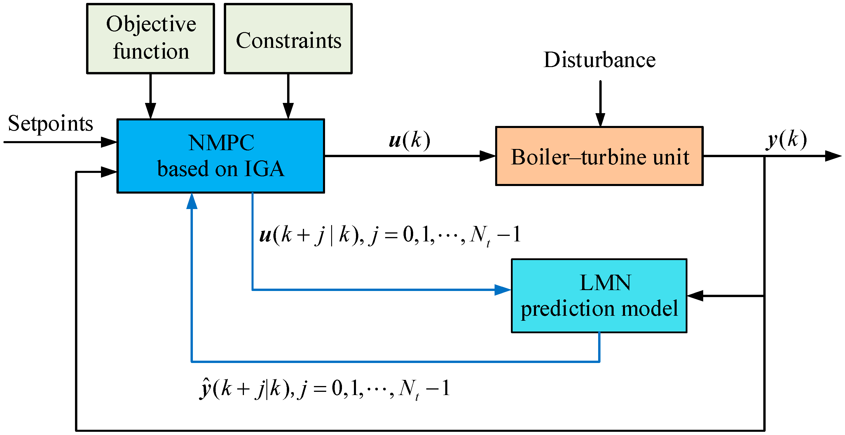
4. Nonlinear Predictive Control Based on IGA Optimization

4.1. State-Space Representation of the Prediction Model

Define $\mathit{x}\left(k\right)={\left[{\mathit{y}}^T\left(k\right),\dots ,{\mathit{y}}^T\left(k-n_A+1\right),\dots ,{\mathit{u}}^T\left(k-1\right),\dots ,{\mathit{u}}^T\left(k-n_B\right)\right]}^T$, then the identified LMN global model (7) can be transformed into the following time-varying linear state-space model:

$$\begin{array}{l}\mathit{x}\left(k+1\right)=\mathit{A}\left(k\right)\mathit{x}\left(k\right)+\mathit{B}\left(k\right)\mathit{u}\left(k\right)\hfill \\ \mathit{y}\left(k\right)=\mathit{C}\mathit{x}\left(k\right)\hfill \end{array}$$

(8)

where $\mathit{A}\left(k\right)=\left[\begin{array}{cccccccc}{\widehat{\mathit{A}}}_1\left(k\right)& \cdots & {\widehat{\mathit{A}}}_{n_A-1}\left(k\right)& {\widehat{\mathit{A}}}_{n_A}\left(k\right)& {\widehat{\mathit{B}}}_1\left(k\right)& \cdots & {\widehat{\mathit{B}}}_{n_B-1}\left(k\right)& {\widehat{\mathit{B}}}_{n_B}\left(k\right)\\ \mathbf{I}& \cdots & \mathbf{O}& \mathbf{O}& \mathbf{O}& \cdots & \mathbf{O}& \mathbf{O}\\ ⋮& \ddots & ⋮& ⋮& ⋮& \ddots & ⋮& ⋮\\ \mathbf{O}& \cdots & \mathbf{I}& \mathbf{O}& \mathbf{O}& \cdots & \mathbf{O}& \mathbf{O}\\ \mathbf{O}& \cdots & \mathbf{O}& \mathbf{O}& \mathbf{O}& \cdots & \mathbf{O}& \mathbf{O}\\ \mathbf{O}& \cdots & \mathbf{O}& \mathbf{O}& \mathbf{I}& \cdots & \mathbf{O}& \mathbf{O}\\ ⋮& \ddots & ⋮& ⋮& ⋮& \ddots & ⋮& ⋮\\ \mathbf{O}& \cdots & \mathbf{O}& \mathbf{O}& \mathbf{O}& \cdots & \mathbf{I}& \mathbf{O}\end{array}\right]$; $\mathit{B}\left(k\right)=\left[\begin{array}{c}{\widehat{\mathit{B}}}_0\left(k\right)\\ \mathbf{O}\\ ⋮\\ \mathbf{O}\\ \mathbf{I}\\ \mathbf{O}\\ ⋮\\ \mathbf{O}\end{array}\right]$; $\mathit{C}=\left[\begin{array}{cccc}\mathbf{I}& \mathbf{O}& \cdots & \mathbf{O}\end{array}\right]$; ${\widehat{\mathit{A}}}_j\left(k\right)=-{\displaystyle \sum _{i=1}^M{\rho }_i\left(\mathit{\varphi }\left(k\right)\right){\mathit{A}}_{ij}},j=1,\cdots ,n_A$; ${\widehat{\mathit{B}}}_j\left(k\right)={\displaystyle \sum _{i=1}^M{\rho }_i\left(\mathit{\varphi }\left(k\right)\right){\mathit{B}}_{ij}},j=1,\cdots ,n_B$.

Through the above transformation, multiple identified single-output local models are combined into a global multi-input multi-output (MIMO) state-space model, and the state of the system at future instants can be predicted:

$$\begin{array}{l}\mathit{x}\left(k+1|k\right)=\mathit{A}\left(k\right)\mathit{x}\left(k\right)+\mathit{B}\left(k\right)\mathit{u}\left(k|k\right)\\ \mathit{x}\left(k+2|k\right)=\mathit{A}\left(k+1\right)\mathit{A}\left(k\right)\mathit{x}\left(k\right)+\mathit{A}\left(k+1\right)\mathit{B}\left(k\right)\mathit{u}\left(k|k\right)+\mathit{B}\left(k+1\right)\mathit{u}\left(k+1|k\right)\\ ⋮\\ \mathit{x}\left(k+N_t|k\right)=\mathit{A}\left(k+N_t-1\right)\cdots \mathit{A}\left(k\right)\mathit{x}\left(k\right)+\mathit{A}\left(k+N_t-1\right)\cdots \mathit{A}\left(k+1\right)\mathit{B}\left(k\right)\mathit{u}\left(k|k\right)\\ +\mathit{A}\left(k+N_t-1\right)\cdots \mathit{A}\left(k+2\right)\mathit{B}\left(k+1\right)\mathit{u}\left(k+1|k\right)+\cdots \\ +\mathit{B}\left(k+N_t-1\right)\mathit{u}\left(k+N_t-1|k\right)\\ ⋮\end{array}$$

(9)

Note that the state transition matrix $\mathit{A}\left(k+j\right)$ and $\mathit{B}\left(k+j\right)$ are time-varying during the prediction horizon following the change of the scheduling vector $\mathit{\varphi }\left(k+j\right)$ at each sampling instant. As a result, the prediction error can be effectively reduced. Compared with the general state-space model obtained by piecewise linearization of the nonlinear system, this model may have two advantages: first, it can express the original system more accurately; second, the state observer does not need to be designed, because every state element in $\mathit{x}\left(k\right)$ can be measured.

4.2. Nonlinear Optimization Problem Formulation

Mayne and Rawlings [40] analyzed the stability of many predictive control algorithms and established a design framework for MPC to guarantee the stability of a closed-loop system, which consists of three components: local stabilizing controller, terminal constraint set, and terminal cost function; and proved that the stability of MPC can be guaranteed when certain conditions are satisfied. Rawlings and Mayne [41] showed that addition of a terminal cost does not materially affect the optimal control problem, while addition of a terminal constraint, which is a state constraint, may have a significant effect. Therefore, it is considered if the terminal constraint can be omitted without affecting stability. A reasonably simple procedure is to replace the terminal constraint by a terminal cost that is sufficiently large to ensure automatic satisfaction of the terminal constraint. The predictive controller in this paper will be designed based on this guaranteed stability formulation.

4.2.1. Objective Function

To achieve an optimal dynamic performance while guaranteeing the stability of the system, the following objective function or performance index can be adopted:

$$\begin{array}{l}J\left(k\right)={\displaystyle \sum _{j=0}^{N_t-1}\left[{\left(\mathit{x}\left(k+j+1|k\right)-{\mathit{x}}_r\right)}^T\mathit{Q}\left(\mathit{x}\left(k+j+1|k\right)-{\mathit{x}}_r\right)+{\left(\mathit{u}\left(k+j|k\right)-{\mathit{u}}_r\right)}^T\mathit{R}\left(\mathit{u}\left(k+j|k\right)-{\mathit{u}}_r\right)\right]}\\ +{\beta }_t\mathit{\Psi }\left(\mathit{x}\left(k+N_t+1|k\right)-{\mathit{x}}_r\right)\end{array}$$

(10)

where $N_t$ is the prediction horizon; $\mathit{Q}={\mathit{Q}}^T>0$ and $\mathit{R}={\mathit{R}}^T>0$ are symmetric weighting matrices of the state and control input tracking errors; $\mathit{x}\left(k+j+1|k\right)$ is the predicted state at time instant $k+j+1|k$ and $\mathit{u}\left(k+j|k\right)$ is the control action at future instant $k+j$ to be optimized at current instant $k$; ${\mathit{x}}_r$ and ${\mathit{u}}_r$ are the steady-state targets of state and control inputs, respectively. The last term is the terminal cost with weight coefficient ${\beta }_t\ge 1$, and the terminal cost function is defined as

$$\mathit{\Psi }\left(\mathit{x}\left(k+N_t+1|k\right)-{\mathit{x}}_r\right)={\left(\mathit{x}\left(k+N_t+1|k\right)-{\mathit{x}}_r\right)}^T\mathit{P}\left(k\right)\left(\mathit{x}\left(k+N_t+1|k\right)-{\mathit{x}}_r\right)$$

(11)

where $\mathit{P}(k)$ is a symmetric positive weighting matrix, called a terminal penalty matrix.

Considering the state and input constraints of the system, the optimization problem to be solved at each sampling instant can be described as follows:

$$\underset{U}{\min }J\left(k\right)$$

(12)

s.t. Eq. (8)

$${\mathit{u}}_{\min }\le \mathit{u}\left(k+j|k\right)\le {\mathit{u}}_{\max },j=0,1,\cdots ,N_t-1$$

$$\Delta {\mathit{u}}_{\min }\le \Delta \mathit{u}\left(k+j|k\right)\le \Delta {\mathit{u}}_{\max },j=0,1,\cdots ,N_t-1$$

where $\mathit{U}={\left[{\mathit{u}}^T\left(k|k\right),\cdots ,{\mathit{u}}^T\left(k+N_t-1|k\right)\right]}^T$ is the control input sequence to be optimized.

The terminal constraint is not included in (12) for the reason that if β_t is sufficiently large, the terminal constraint can be implicitly satisfied [41]. The introduction of terminal cost can make the objective function (10) decay over time, so that the stability of the predictive control system is guaranteed. Meanwhile, the online computational burden for optimization can be decreased as a result so that a small N_t can be adopted in (10).

4.2.2. Steady-State Target

The equilibrium state and associated steady-state control input ${\mathit{x}}_r$ and ${\mathit{u}}_r$ of the system corresponding to the desired output ${\mathit{y}}_r$ can be obtained by solving the following algebraic equations online:

$$\{\begin{array}{l}{\mathit{x}}_r=\mathit{A}\left(k\right){\mathit{x}}_r+\mathit{B}\left(k\right){\mathit{u}}_r\\ {\mathit{y}}_r=\mathit{C}{\mathit{x}}_r+\mathit{h}\left(\mathit{y}\left(k\right)-\mathit{y}\left(k|k-1\right)\right)\end{array}$$

(13)

where h is the feedback correction coefficient vector. Because the target state and control input are feedback corrected by prediction error $\mathit{y}\left(k\right)-\mathit{y}\left(k|k-1\right)$ at each step, the offset-free output tracking can be achieved even in the presence of model uncertainty.

4.2.3. Terminal Penalty Matrix

For a nonlinear system, generally the nonlinear model is first linearized at a certain equilibrium point (e.g., the origin), and then the solution of the algebraic Riccati equation corresponding to the linear model is obtained as a weight matrix P. However, for the tracking problem where the setpoint of output is changing, it is obviously not feasible to determine P according to the one fixed equilibrium point. To this end, an automatic switching method of the matrix P with tracking trajectory is presented here.

The local linear model $L{M}_i\left(i=1,\dots ,M\right)$ of the identified LMN can be described in the form of state-space:

$$\{\begin{array}{l}\mathit{x}\left(k+1\right)={\mathit{A}}_{m,i}\mathit{x}\left(k\right)+{\mathit{B}}_{m,i}\mathit{u}\left(k\right)\\ \mathit{y}\left(k\right)={\mathit{C}}_{m,i}\mathit{x}\left(k\right)\end{array}$$

(14)

where ${\mathit{A}}_{m,i}$, ${\mathit{B}}_{m,i}$, and ${\mathit{C}}_{m,i}$ are constant matrices.

Then, the solution ${\mathit{P}}_i$ of the following algebraic Riccati equation for each local linear model and the feedback gain coefficient matrix ${\mathit{K}}_i$ of the corresponding local controller $\mathit{u}={\mathit{K}}_i\mathit{x}$ can be obtained offline by a linear quadratic regulator (LQR):

$${\mathit{P}}_i={\mathit{A}}_{m,i}^T{\mathit{P}}_i{\mathit{A}}_{m,i}-{\mathit{A}}_{m,i}^T{\mathit{P}}_i{\mathit{B}}_{m,i}\left({\mathit{B}}_{m,i}^T{\mathit{P}}_i{\mathit{B}}_{m,i}+\mathit{R}\right){\mathit{B}}_{m,i}^T{\mathit{P}}_i{\mathit{A}}_{m,i}+\mathit{Q}$$

(15)

$${\mathit{K}}_i=-\left({\mathit{B}}_{m,i}^T{\mathit{P}}_i{\mathit{B}}_{m,i}+\mathit{R}\right){\mathit{B}}_{m,i}^T{\mathit{P}}_i{\mathit{A}}_{m,i}$$

(16)

Note that the fictitious local controllers are only used to determine $\mathit{P}\left(k\right)$ and help to improve IGA in the next section.

In online optimization, according to the current scheduling vector $\mathit{\varphi }\left(k\right)$, the matrix ${\mathit{P}}_{\sigma (k)}$ corresponding to the local model with the largest validity is selected as the current terminal penalty matrix $\mathit{P}\left(k\right)$,

$$\mathit{P}\left(k\right)={\mathit{P}}_{\sigma (k)}, \sigma \left(k\right)=\arg \underset{i\in \{1,2,\cdots ,M\}}{\max }{\rho }_i\left(\mathit{\varphi }\left(k\right)\right)$$

(17)

When the setpoint changes, the system can automatically adjust the weight matrix of the terminal cost (11) in the objective function (10) according to the scheduling vector reflecting the current operating condition, which is equivalent to automatically adjusting the fictitious terminal constraint set, thus guaranteeing the stability of the system.

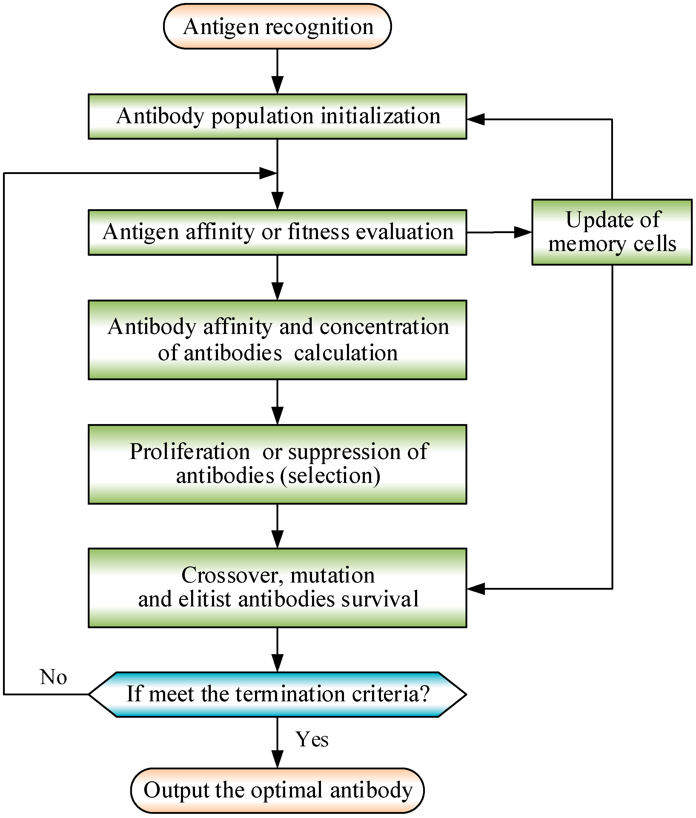
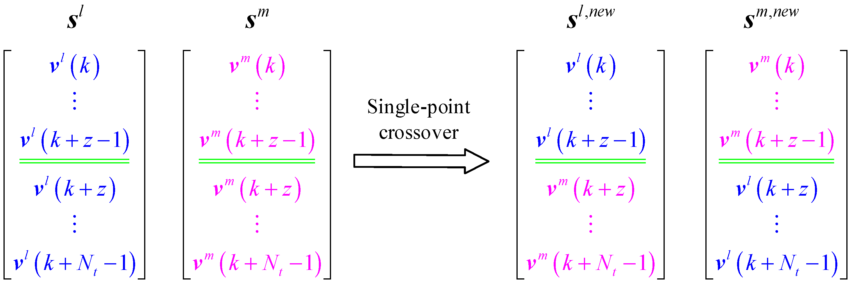
4.3. Receding Horizon Optimization Based on IGA

Evolutionary algorithms (EAs) have shown their superiority in solving nonlinear optimization problem [5,7,16,42]. Comparing with other EAs, the immune genetic algorithm (IGA) can avoid premature convergence and guarantee the population diversity, thus can rapidly converge to the global optimum [42,43,44,45,46,47]. So, an IGA proposed in [47] is modified in this paper to perform the receding horizon optimization of the nonlinear predictive controller. The IGA takes the problem to be solved as an antigen and the feasible solutions as antibodies. The basic flowchart of IGA is shown in Figure 5. At each sampling instant, IGA is used to solve the constrained nonlinear optimization problem (12) online to obtain the optimal control sequence $\left\{{\mathit{u}}^{*}\left(k+j|k\right),j=0,\cdots ,N_t-1\right\}$ which can minimize the objective function (10).

The objective function (10) that reflects the control performance is represented as the antigen, and the antibodies represent the feasible solutions to the problem (i.e., the candidate control inputs to be applied to the system). The fitness of the feasible solutions is reflected by the affinity of antibodies and antigen. During the execution of the algorithm, the antibodies with lower affinity may be replaced by new antibodies with a higher probability. For the convenience of description, we denote the unknown future control actions $\left\{\mathit{u}\left(k+j|k\right),j=0,\dots ,N_t-1\right\}$ as $\left\{\mathit{v}\left(k+j\right),j=0,\dots ,N_t-1\right\}$ to distinguish them from the past control inputs which are known. Antibodies are encoded with real numbers. For the multivariable system with $n_i$ inputs, any antibody ${\mathit{s}}^l$ in the population can be expressed as:

$${\mathit{s}}^l=[{\mathit{v}}_1^l,{\mathit{v}}_2^l,\dots ,{\mathit{v}}_{n_i}^l]=\left[\begin{array}{c}{\mathit{v}}^l\left(k\right)\\ {\mathit{v}}^l\left(k+1\right)\\ ⋮\\ {\mathit{v}}^l\left(k+N_t-1\right)\end{array}\right]=\left[\begin{array}{cccc}{v}_1^l\left(k\right)& v_2^l\left(k\right)& \cdots & v_{n_i}^l\left(k\right)\\ v_1^l\left(k+1\right)& v_2^l\left(k+1\right)& \cdots & v_{n_i}^l\left(k+1\right)\\ ⋮& ⋮& \ddots & ⋮\\ v_1^l\left(k+N_t-1\right)& v_2^l\left(k+N_t-1\right)& \cdots & v_{n_i}^l\left(k+N_t-1\right)\end{array}\right]$$

(18)

where ${\mathit{v}}_i^l={\left[v_i^l\left(k\right),v_i^l\left(k+1\right),\dots ,v_i^l\left(k+N_t-1\right)\right]}^T$ is column vector, $i=1,\cdots ,n_i$; ${\mathit{v}}^l\left(k+j\right)=\left[v_1^l\left(k+j\right),v_2^l\left(k+j\right),\dots ,v_{n_i}^l\left(k+j\right)\right]$ is row vector, $j=0,\cdots ,N_t-1$.

At the current instant k, online optimization based on IGA consists of the following steps:

Step 1. (Antibody population initialization): An initial population with $N_L$ antibodies (candidate control sequences) will be generated. Because of the receding horizon principle of predictive control, memory cells retained from the previous sampling period can be used to generate some excellent initial antibodies in current instant. The existing antibodies in the memory cells are activated, and the original genes in each active antibody are moved forward so that the original first gene is omitted, and then the following control input produced by the fictitious local controller is supplemented as the last gene,

$${\mathit{v}}^l\left(k+N_t-1\right)={\mathit{K}}_{\sigma (k-1)}\mathit{x}\left(k+N_t-1|k-1\right)$$

(19)

where the subscript $\sigma \left(k-1\right)$ of feedback gain coefficient matrix $\mathit{K}$ is as defined in (17).

The remaining antibodies in the initial population are randomly generated, but they need to satisfy the control input constraints. Assume that $\mathit{u}\left(k-1\right)=\left[u_1\left(k-1\right),u_2\left(k-1\right),\cdots ,u_{n_i}\left(k-1\right)\right]$ is the control vector that has been applied to the process at past instant $k-1$, the candidate control inputs at instant $k$ can be selected as follows:

$$v_i^l\left(k\right)=\min \left(u_{i\max },\max \left(u_{i\min },u_i\left(k-1\right)+r_0\Delta u_{i\max }\right)\right), 1\le i\le n_i$$

(20)

and

$$v_i^l\left(k+j\right)=\min \left(u_{i\max },\max \left(u_{i\min },v_i\left(k+j-1\right)+r_0\Delta u_{i\max }\right)\right), 1\le j\le N_t-1$$

(21)

where $r_0$ is a random number in the interval $[-1,1]$ and is regenerated every time it is used.

Step 2. (Antigen affinity or fitness evaluation): Each antibody in the population is applied to the prediction model (8). The predicted state $\mathit{x}\left(k+j|k\right)$ and output $\mathit{y}\left(k+j|k\right)\left(j=0,1,\dots ,N_t-1\right)$ can be obtained based on (8) and (9). The target state and input $\left({\mathit{x}}_r,{\mathit{u}}_r\right)$ are obtained by solving (13). Evaluate the objective function $J\left(k\right)$ for all antibodies by (10) and then calculate their antigen affinity:

$${\left(A_g\right)}_l=\frac{1}{1+J\left(k\right)}$$

(22)

Step 3. (Update of memory cells): Since the number of memory cells $N_{rem}$ is limited, the new antibody with the highest antigen affinity in the population will compete with the antibodies in memory cells. The old antibody will be replaced if its fitness is lower than the new fittest antibody, while their affinity is the highest in memory cells, so as to maintain the original size of the memory cells.

Step 4. (Proliferation and suppression of antibodies): The affinity between two antibodies ${\mathit{s}}^l$ and ${\mathit{s}}^m$ is calculated as

$${\left(A_b\right)}_{lm}=\frac{1}{1+H{S}_{lm}}$$

(23)

where $H{S}_{lm}=\sqrt{{\displaystyle \sum _{i=1}^{n_i}{\displaystyle \sum _{j=0}^{N_t-1}{\left(v_i^l\left(k+j\right)-v_i^m\left(k+j\right)\right)}^2}}}$ is the distance between two antibodies ${\mathit{s}}^l$ and ${\mathit{s}}^m$. The higher affinity represents the more similar two antibodies.

The concentration $C_l$ of each antibody ${\mathit{s}}^l$ represents the proportion of similar antibodies of ${\mathit{s}}^l$ in the whole population, which can be calculated by

$$C_l=\frac{1}{N_L}{\displaystyle \sum _{m=1}^{N_L}n}{c}_{lm},n{c}_{lm}=\{\begin{array}{cc}1,& {\left(A_b\right)}_{lm}\ge \xi \\ 0,& \mathrm{otherwise}\end{array}$$

(24)

where ξ is called an affinity coefficient, which means the limit of the similarity. In general, 0.9 ≤ ξ ≤ 1.

The selection criteria of each antibody ${\mathit{s}}^l$, which takes into account both its antigenic affinity ${\left(A_g\right)}_l$ and concentration $C_l$, is as follows:

$$E_l={\lambda }_c{\left(A_g\right)}_l+\left(1-{\lambda }_c\right)e^{-{\mu }_c{C}_l}$$

(25)

where ${\lambda }_c$ and ${\mu }_c$ are weighting coefficients. This criteria promotes the proliferation of the antibody with high antigen affinity, and suppresses the antibody with high concentration, which can enhance the diversity of population. In general, ${\lambda }_c=0.7$ and ${\mu }_c=1.25$.

Step 5. (Crossover and mutation operations): The antibodies are selected by roulette wheel based on criteria (25). Then a new-generation antibody population is generated through mutation and crossover operators, while the elite antibodies in the memory cells will survive into the new generation to evolve.

For each antibody, a random number $r_1\in [0,1]$ is generated. If $r_1<P_c$ (crossover probability), this particular antibody will be selected to perform the crossover. For each crossover pair, single-point crossover and uniform crossover operations will be implemented with equal probability to keep the population diversity. We have tested a variety of crossover methods in our algorithm design and found that the combination of these two crossover methods can achieve better control performance, indicating that diversity and convergence of the population are better guaranteed.

Suppose a pair of antibodies ${\mathit{s}}^l$ and ${\mathit{s}}^m$ are selected for crossover, the single-point crossover operation is shown in Figure 6.

The position of the crossover point $z$ is randomly generated in integers between 1 and $N_t-1$. Two new antibodies ${\mathit{s}}^{l,new}$ and ${\mathit{s}}^{m,new}$ will be produced by shifting the parent genes following the crossover point $z$, but they might be infeasible offspring if the constraint on control move is not satisfied after crossover. So, a correction mechanism is designed for the new offspring. Taking ${\mathit{s}}^{l,new}$ as an example, let $dc=v_i^m\left(k+z\right)-v_i^l\left(k+z-1\right)$, then its genes following the crossover point $z$, $v_i^m\left(k+z+j\right)\left(0\le j\le N_t-z-1\right)$ can be corrected as

$$v_i^m\left(k+z+j\right)=\{\begin{array}{cc}{v}_i^m\left(k+z+j\right)-\left(dc-\Delta u_{i\max }\right),& \mathrm{if}dc>\Delta u_{i\max }\\ v_i^m\left(k+z+j\right)-\left(dc+\Delta u_{i\max }\right),& \mathrm{if}dc<-\Delta u_{i\max }\end{array}$$

(26)

For the uniform crossover, each gene in the two offspring antibodies ${\mathit{s}}^{l,new}$ and ${\mathit{s}}^{m,new}$ can be obtained by performing the following operation on the two genes at the same position $v_i^l(k+j)$ and $v_i^m\left(k+j\right), \left(1\le i\le n_i,0\le j\le N_t-1\right)$ in the two parent antibodies:

$$\{\begin{array}{cc}{\mathit{s}}^{l,new}:& v_i^{l,new}\left(k+j\right)=r_c\cdot v_i^l\left(k+j\right)+\left(1-r_c\right)v_i^m\left(k+j\right)\\ {\mathit{s}}^{m,new}:& v_i^{m,new}\left(k+j\right)=r_c\cdot v_i^m\left(k+j\right)+\left(1-r_c\right)v_i^l\left(k+j\right)\end{array}$$

(27)

where $r_c$ is a random number between 0 and 1.

For every gene $v_i^l\left(k+j\right)$ of each antibody ${\mathit{s}}^l$ in the population, a random number $r_b\in [0,1]$ is generated. If $r_b<P_m$(mutation probability), this particular gene will undergo the mutation, otherwise it will remain unchanged. To ensure that the mutated antibody is a feasible solution, it is necessary to define the variation region of $v_i^l(k+j)$. The upper bound $b_u\left(j\right)$ and lower bound $b_l\left(j\right)$ are defined as:

$$b_u\left(j\right)=\{\begin{array}{cc}\min \left(\Delta u_{i\max }+u_i\left(k-1\right),\Delta u_{i\max }+v_i^l\left(k+1\right),u_{i\max }\right),& j=0\\ \min \left(\Delta u_{i\max }+v_i^l\left(k+j-1\right),\Delta u_{i\max }+v_i^l\left(k+j+1\right),u_{i\max }\right),& 0<j<N_t-1\\ \min \left(\Delta u_{i\max }+v_i^l\left(k+j-1\right),u_{i\max }\right),& j=N_t-1\end{array}$$

(28)

$$b_l\left(j\right)=\{\begin{array}{cc}\max \left(-\Delta u_{i\max }+u_i\left(k-1\right),-\Delta u_{i\max }+v_i^l\left(k+1\right),u_{i\min }\right),& j=0\\ \max \left(-\Delta u_{i\max }+v_i^l\left(k+j-1\right),-\Delta u_{i\max }+v_i^l\left(k+j+1\right),u_{i\min }\right),& 0<j<N_t-1\\ \max \left(-\Delta u_{i\max }+v_i^l\left(k+j-1\right),u_{i\min }\right),& j=N_t-1\end{array}$$

(29)

Then, the new mutated antibody gene $v_i^{l,new}\left(k+j\right)$ can be obtained after the generation of a random number $b_c\left(j\right)\in \left[b_l\left(j\right),b_u\left(j\right)\right]$,

$$v_i^{l,new}\left(k+j\right)=\{\begin{array}{cc}{v}_i^l\left(k+j\right),& r_b\ge P_m\\ b_c\left(j\right),& r_b<P_m\end{array}$$

(30)

In order to further improve the performance of IGA, $P_c$ and $P_m$ are adaptively adjusted following the evolutionary process,

$$P_c=\{\begin{array}{cc}{P}_{c,u}-\frac{\left(P_{c,u}-P_{c,l}\right)\left({\left(A_g\right)}_{l,b}-{\left(A_g\right)}_{avg}\right)}{{\left(A_g\right)}_{\max }-{\left(A_g\right)}_{avg}},& {\left(A_g\right)}_{l,b}\ge {\left(A_g\right)}_{avg}\\ P_{c,u},& {\left(A_g\right)}_{l,b}<{\left(A_g\right)}_{avg}\end{array}$$

(31)

$$P_m=\{\begin{array}{cc}{P}_{m,u}-\frac{\left(P_{m,u}-P_{m,l}\right)\left({\left(A_g\right)}_l-{\left(A_g\right)}_{avg}\right)}{{\left(A_g\right)}_{\max }-{\left(A_g\right)}_{avg}}& {\left(A_g\right)}_l\ge {\left(A_g\right)}_{avg}\\ P_{m,u}& {\left(A_g\right)}_l<{\left(A_g\right)}_{avg}\end{array}$$

(32)

where ${\left(A_g\right)}_{\max }$ and ${\left(A_g\right)}_{avg}$ are, respectively, the maximum and average antigen affinity of the population; ${\left(A_g\right)}_{l,b}$ is the higher antigen affinity of the two antibodies involved in crossover; ${\left(A_g\right)}_l$ is the antigenic affinity of the antibody to be mutated; $P_{c,u}$ and $P_{c,l}$ are the upper and lower bounds of crossover probability, respectively; and $P_{m,u}$ and $P_{m,l}$ are the upper and lower bounds of mutation probability, respectively. The bounds $P_{c,u}=0.9$, $P_{c,l}=0.6$, $P_{m,u}=0.1$, and $P_{m,l}=0.01$ are chosen in this paper.

Step 6. (Termination criteria): Step 2 to Step 5 are repeated until one of the following three termination criteria is met: (1) The antigen affinity of the fittest antibody is one or very close to one, which means the optimal solution has been found; (2) the maximum antigen affinity of the population is not increased in continuous $N_w$ iterations; or (3) the allowed maximum number of iterations or computation time has been expired. Generally, $N_w$ is chosen to be three to five, or about 10% of the allowed maximum number of iterations. The designed termination criteria can avoid redundant iteration and make it possible to obtain the optimal or suboptimal control in real time.

4.4. Implementation of the NMPC based on an LMN and IGA

Application of the proposed NMPC scheme to the B-T unit can be summarized as Algorithm 1, which includes two parts: offline model identification and online optimization control.

Algorithm 1. Implementation procedure of the NMPC based on an LMN and IGA

Off-line part: S01. The LMN model of the nonlinear B-T unit is identified based on the data-driven modeling method and converted into the global model shown in (8) as the prediction model; S02. Linear local models in the LMN are converted into the state-space form (13) and the candidate terminal penalty matrix ${\mathit{P}}_i$ and gain matrix ${\mathit{K}}_i$ of the local controller are calculated by (14) and (15) for each local model. S03. The parameters and weighting matrices in the objective function (10)., the parameters in IGA, along with the control and control move constraints are given. Online part: S1. At the current instant k, the scheduling vector $\mathit{\varphi }(k)$ and the current state $\mathit{x}\left(k\right)={\left[{\mathit{y}}^T\left(k\right),\dots ,{\mathit{y}}^T\left(k-n_A+1\right),\dots ,{\mathit{u}}^T\left(k-1\right),\dots ,{\mathit{u}}^T\left(k-n_B\right)\right]}^T$ are obtained according to the measured input and output of the system, forming the optimization problem (12); S2. IGA is used to solve (12) to obtain the optimal or sub-optimal control sequence $\left\{{\mathit{u}}^{*}\left(k+j|k\right),j=0,\cdots ,N_t-1\right\}$; S3. The output of the system is obtained by applying the control input ${\mathit{u}}^{*}\left(k|k\right)$ to the plant; S4. Let $k=k+1$, go to S1 and proceed to the calculation for the next sampling period.

5. Simulation Results

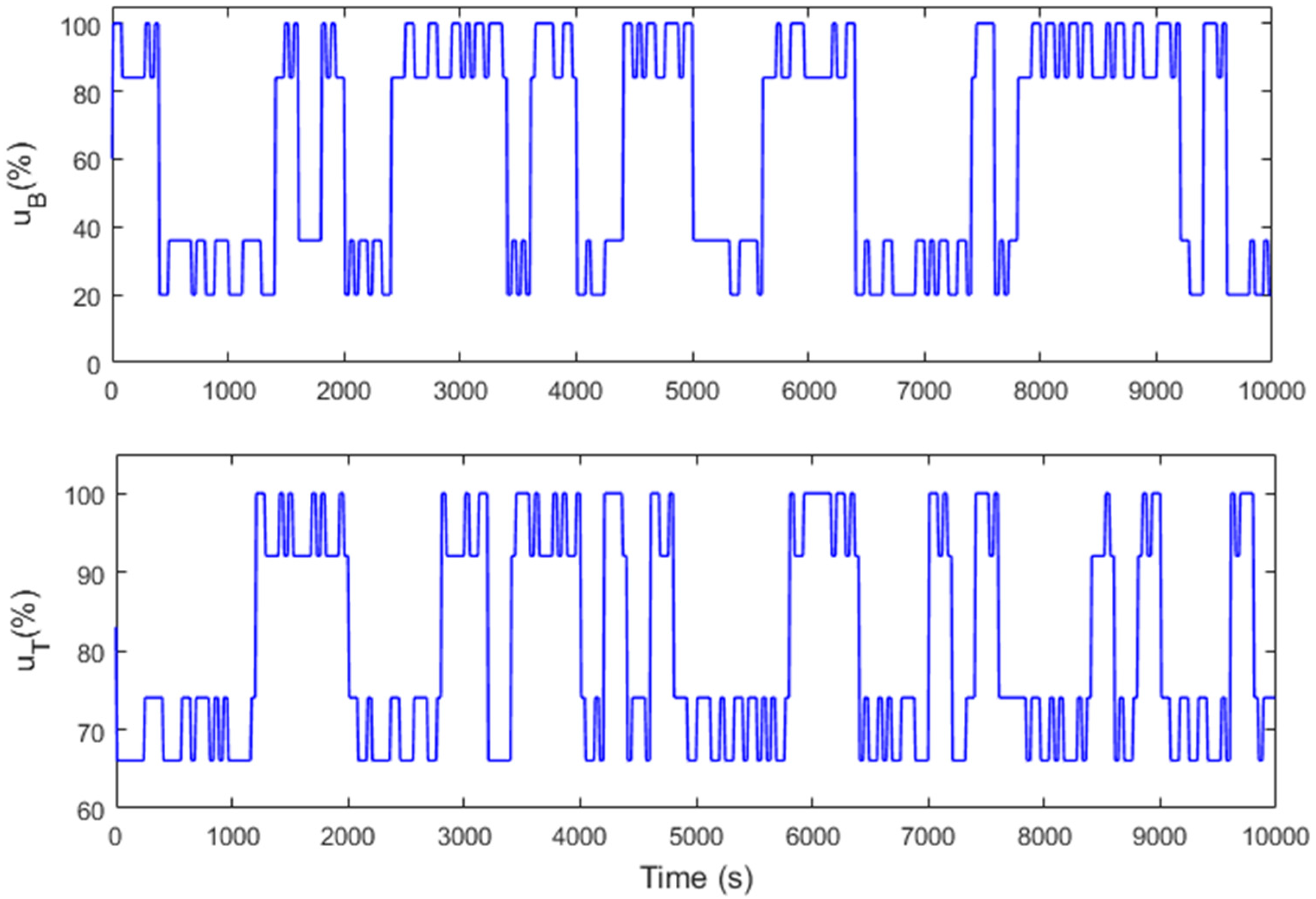
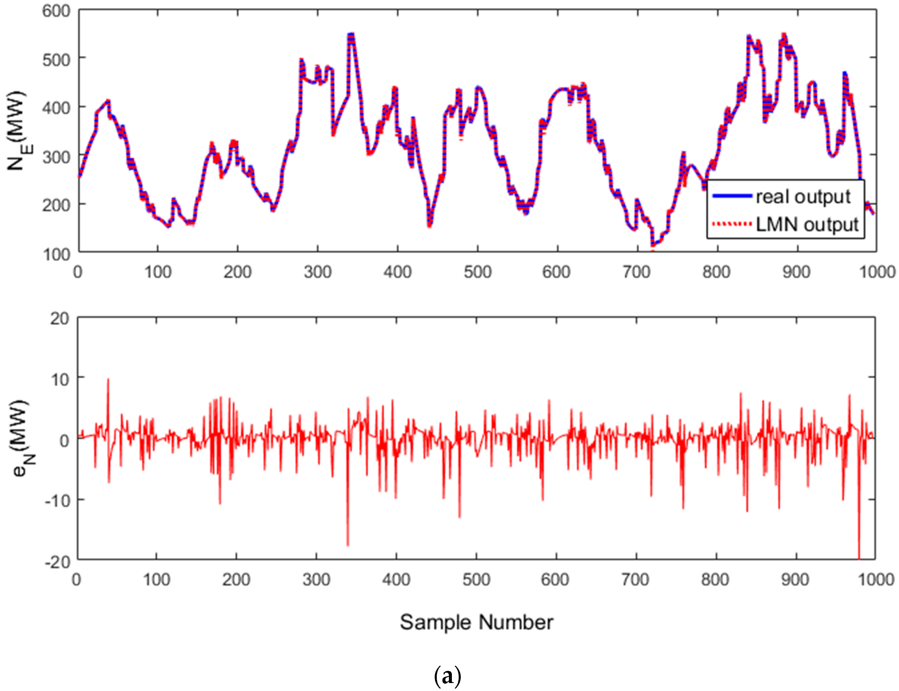
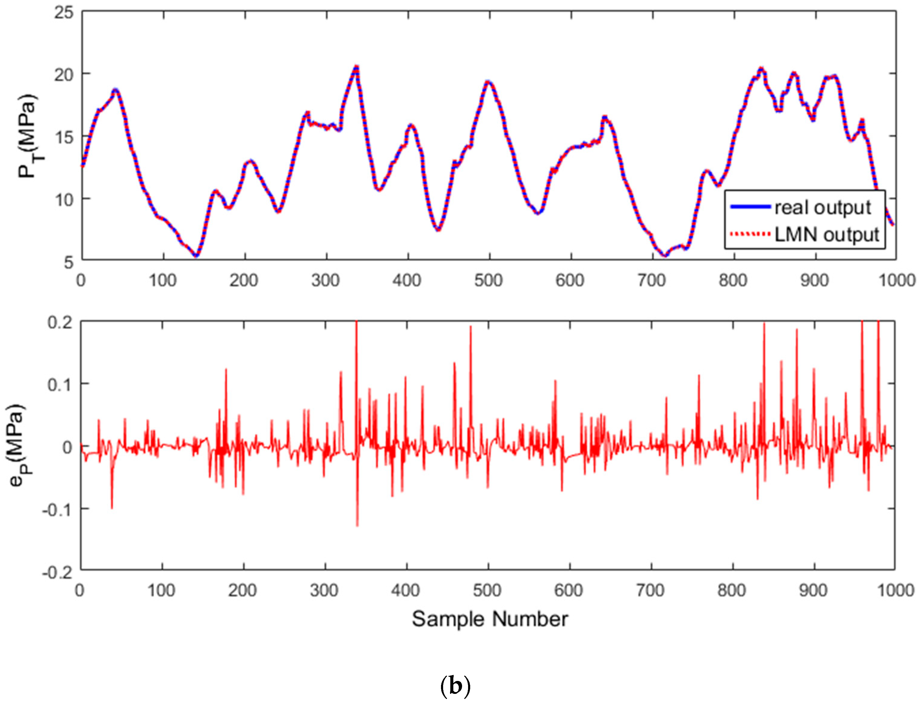
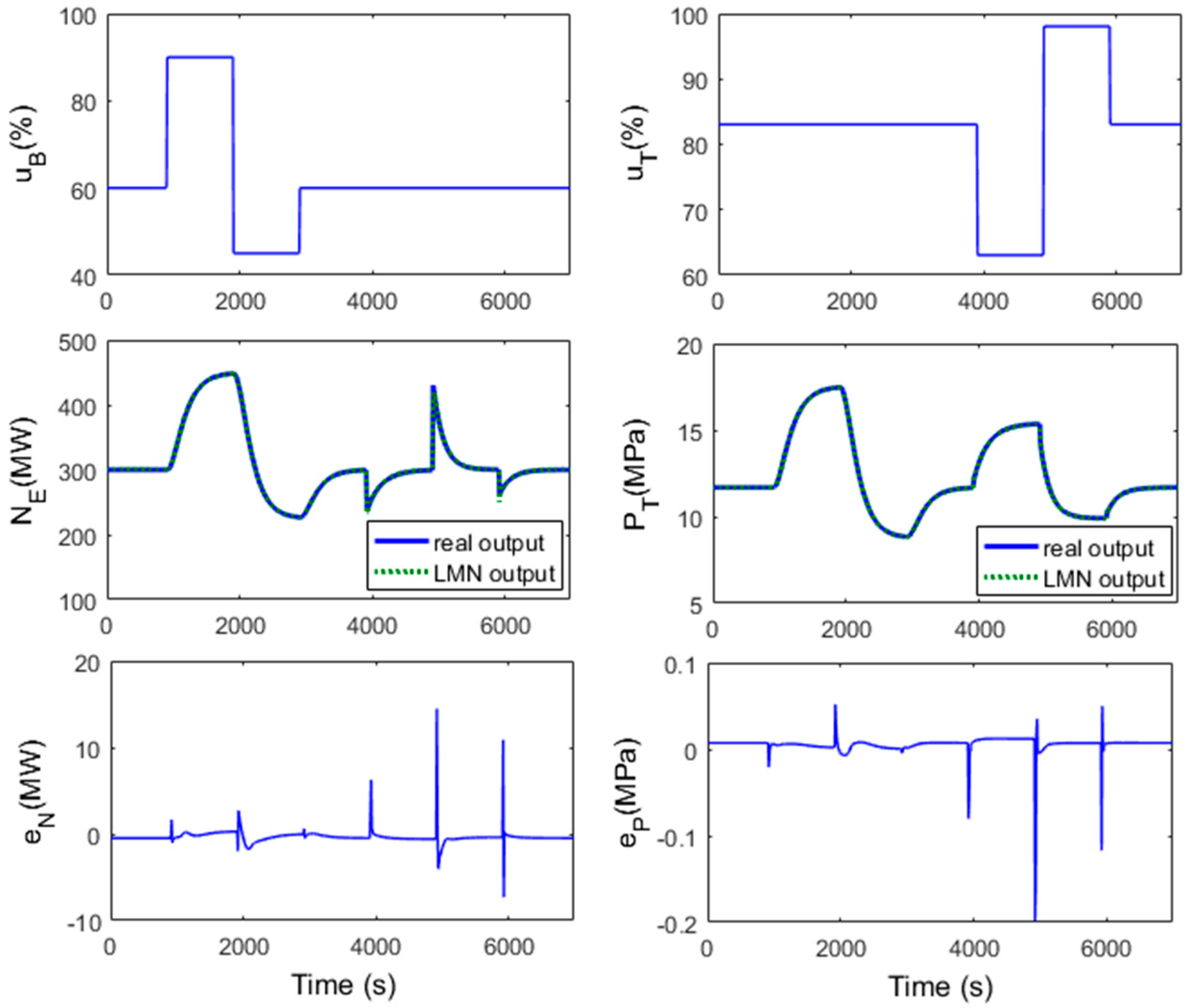
5.1. Model Identification and Test for the B-T Unit

The LMN model of the 500 MW coal-fired B-T unit shown in Figure 1 is identified to provide the prediction mode for the proposed nonlinear predictive control method. In order to fully stimulate the nonlinearity of the B-T unit under different load conditions, two uncorrelated modified pseudo-random sequences are respectively applied to the two manipulated variables $u_B$ and $u_T$ to generate identification data, as shown in Figure 7. The sampling period of the data was 10 s, and 1000 sets of data were recorded as identification data. The low frequency part of the excitation signal can drive the unit to run in the full operating range, while the high frequency part can ensure the unit to be fully excited at local operating points. The corresponding outputs of the unit are shown in Figure 8.

The scheduling vector in LMN can be chosen as $\mathit{\varphi }\left(k\right)=[N_E\left(k-1\right),P_T\left(k-1\right),{u_B\left(k-1\right),u_T\left(k-1\right)]}^T$. The sample data set for identifying the structure of LMN is composed of scheduling vector and output data (i.e., $\left\{{\mathit{z}}_k={\left[{\mathit{\varphi }}^T\left(k\right),N_E\left(k\right),P_T\left(k\right)\right]}^T,k=1,2,\dots ,997\right\}$). The multivariable B-T unit can be decomposed into two single-output subsystems for local model parameter identification. For output power $y_1\left(k\right)=N_E\left(k\right)$, the input vector is selected as ${\mathit{\phi }}_1\left(k\right)=[N_E\left(k-1\right),N_E\left(k-2\right),N_E\left(k-3\right),u_B\left(k-1\right),u_B\left(k-2\right),{u_T\left(k-1\right),u_T\left(k-2\right)]}^T$. For main steam pressure $y_2\left(k\right)=P_T\left(k\right)$, the input vector is selected as:

$${\mathit{\phi }}_2\left(k\right)=[P_T\left(k-1\right),P_T\left(k-2\right),P_T\left(k-3\right),{u_B\left(k-1\right),u_B\left(k-2\right),u_T\left(k-1\right),u_T\left(k-2\right)]}^T.$$

Following the identification procedure shown in Figure 4, the LMN model obtained has satisfactory accuracy when the number of local models in LMN is four, and the model parameters are listed in Appendix A. Normalized root-mean-squared error (NRMSE) can be used as a performance index to test the approximation accuracy of the model,

$$NRMSE\left(y,\widehat{y}\right)=\sqrt{\frac{{\displaystyle {\sum }_{k=1}^N{\left(y\left(k\right)-\widehat{y}\left(k\right)\right)}^2}}{{\displaystyle {\sum }_{i=1}^N{\left(y\left(i\right)-\overline{y}\right)}^2}}},\overline{y}=\frac{1}{N}{\displaystyle \sum _{k=1}^{N}y\left(k\right)}$$

(33)

where $y\left(k\right)$ and $\widehat{y}\left(k\right)$ are the real and model output at the k-th sampling instant, respectively, and $\overline{y}$ is the average of all the real outputs.

The comparison between the model output and the actual output is shown in Figure 8. The model error $e_N$ of output power and $e_P$ of main steam pressure at each sampling instant are also shown in the figure. Obviously, the identified LMN model has very high precision. The NRMSE of output power is 0.031205 and the NRMSE of main steam pressure is 0.00928. We then tested the model with open-loop step response experiments. From the results shown in Figure 9, it can be seen that the resulting LMN model has satisfactory prediction accuracy.

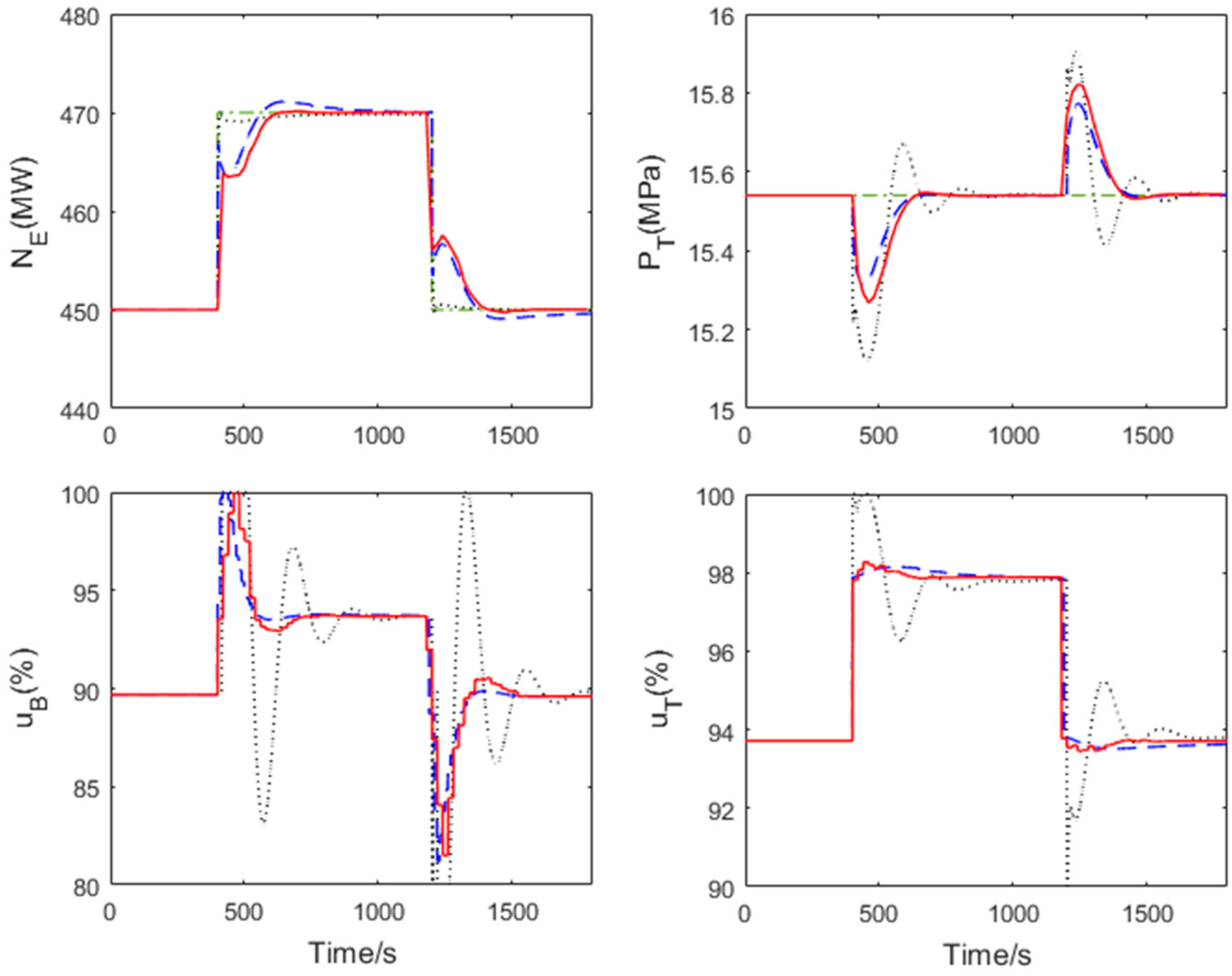
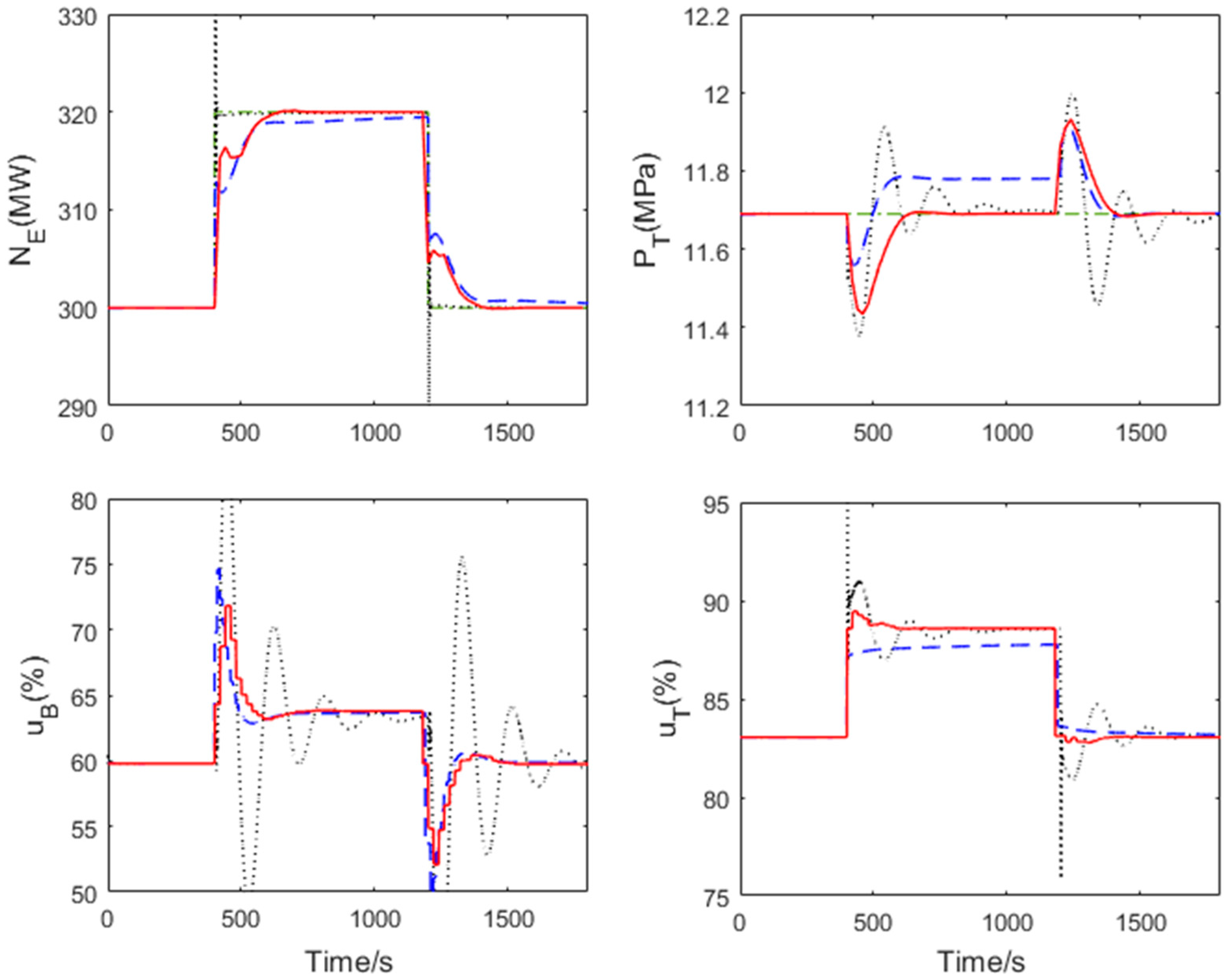
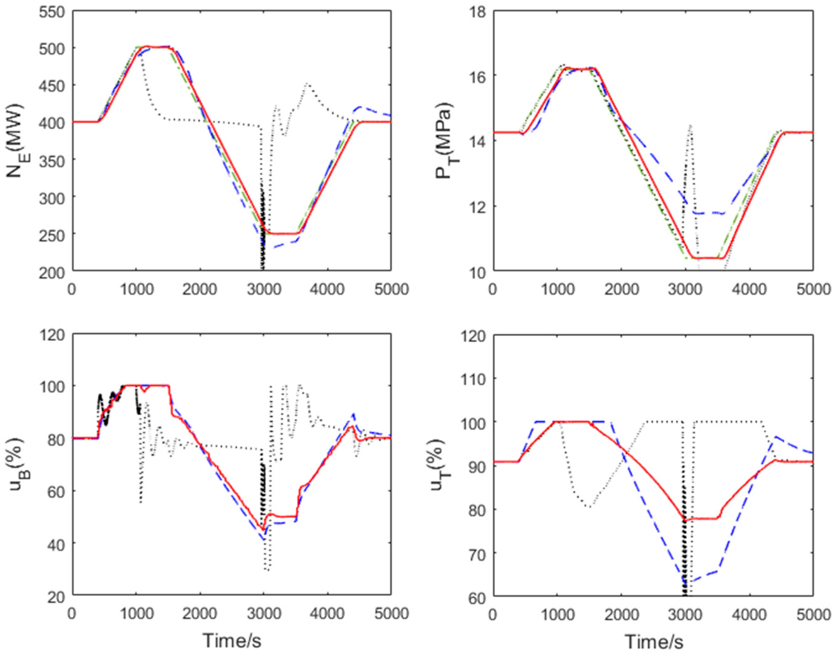
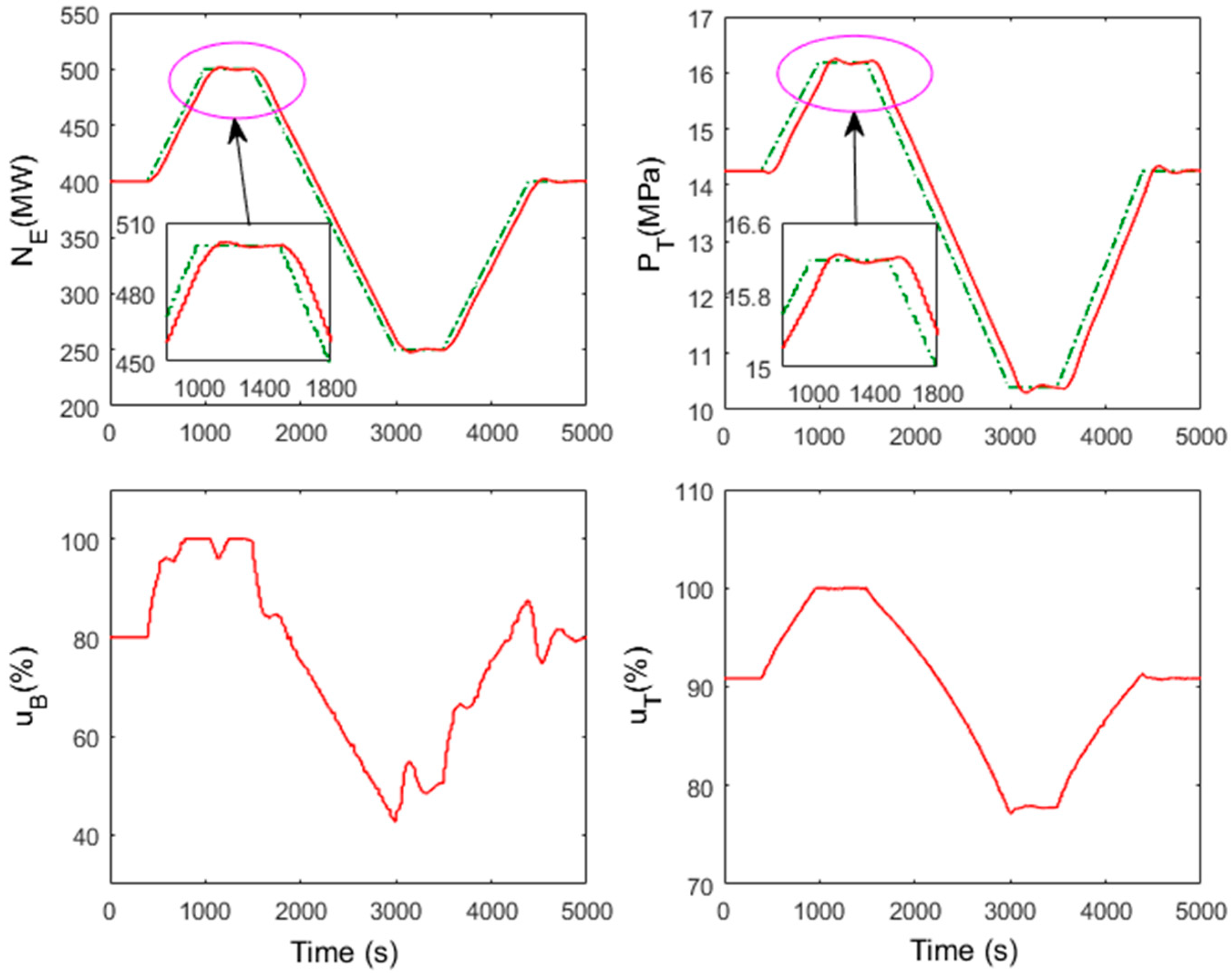
5.2. Validation of the NMPC Control Strategy

The 500 MW coal-fired B-T unit is controlled by the proposed nonlinear predictive control method, which can solve both the control constraints and the nonlinearity caused by the large operating range. By trial and error, the parameters used in the simulations were chosen as: $T_s=10\mathrm{s}$, $N_t=6$, $\mathit{Q}=diag\left\{10,1000,0.1,0.1,0.1,0.1,0.1\right\}$, $\mathit{R}=diag\left\{10,10\right\}$, ${\beta }_t=5$. The parameters in IGA were selected as: $N_L=30$, $N_{gen}=30$, $N_w=4$, other parameters are given in Section 4.3. In order to get the weighting matrix $\mathit{P}$ of the terminal cost function introduced in the objective function (10), each local model LM_i (i = 1,…,4) in the identified LMN is first transformed into a state-space sub-model with state variables $\mathit{x}\left(k\right)=[N_E\left(k\right),P_T\left(k\right),N_E\left(k-1\right),P_T\left(k-1\right),N_E\left(k-2\right),P_T\left(k-2\right),{u_B\left(k-1\right),u_T\left(k-1\right)]}^T$ and outputs $\mathit{y}\left(k\right)={\left[N_E\left(k\right),P_T\left(k\right)\right]}^T$. Then, for each state-space model, a linear quadratic regulator (LQR) method is adopted to obtain the matrix ${\mathit{P}}_i$ as well as gain the ${\mathit{K}}_i$ of the local stabilization controller, where ${\mathit{K}}_i$ and ${\mathit{P}}_i$ corresponding to each local model obtained by the dlqr function in MATLAB are listed in Appendix B.

In the IGA online optimization, at each sampling instant k, the ${\mathit{P}}_i$ corresponding to the local model with the highest validity according to the scheduling vector $\mathit{\varphi }\left(k\right)$ is selected as the current terminal penalty matrix $\mathit{P}\left(k\right)$, and ${\mathit{K}}_i$ is used to create good initial antibodies for IGA. Due to the proper design for each antibody’s initialization and regeneration in IGA, it is ensured that the control inputs $u_B\left(k\right)$ and $u_T\left(k\right)$ always satisfy the constraints (2).

Three case studies which describe the control challenges of the B-T unit are simulated to show the tracking capability of the control system under different operating conditions and its robustness against parameter uncertainty. To verify the performance of the NMPC based on an LMN and IGA, it was compared with two other control strategies, a linear model-based MPC (LMPC) and an inverted decoupling-based PI control [48]. The nominal operating condition is chosen as 90% load condition ($N_E=450\mathrm{MW}$,$P_T=15.54\mathrm{MPa}$), and the nominal linear model is obtained from the nonlinear model (1) based on Taylor series approximation. The LMPC and PI control are well designed based on the nominal linear model. The sampling time and constraint of the LMPC is set as the same as NMPC. By trial and error, the predictive horizon and control horizon of LMPC are set as $N_y=12$ and $N_u=2$, respectively; the output and input weighting matrices are, respectively, set as $diag\left\{10,1000\right\}$ and $diag\left\{10,10\right\}$. After coupling analysis, the PI control system with interaction compensation is designed as the boiler following turbine (BFT) mode, which is able to track the load demand very quickly [2]. The elements of the decoupler are designed based on the nominal transfer function model and then the parameters of the two PI controllers are optimized by using the PID tuner in MATLAB/Simulink.

Case 1: In the first case, we assume that the unit is operating in constant-steam-pressure mode and initially in the steady-state under 90% load condition. At time $t=400\mathrm{s}$, the setpoint of output power $N_E$ is increased by 20 MW, and at time $t=1200\mathrm{s}$, the setpoint of $N_E$ is decreased by 20 MW and returned to 450 MW, while the main steam pressure $P_T$ is kept unchanged. The responses of outputs $N_E$ and $P_T$ as well as the control inputs $u_B$ and $u_T$ are shown in Figure 10. The similar test is also carried out under 60% load condition ($N_E=300\mathrm{MW}$,$P_T=11.69\mathrm{MPa}$), and the results are shown in Figure 11.

It can be seen from Figure 10 and Figure 11 that, for the NMPC, no matter whether under high-load or low-load condition, under the premise of satisfying the constraints on the control action, the output power can be quickly tracked to its setpoint without overshoot, and the fluctuation of main steam pressure is small. The setting time is no more than 250 s and the maximum deviation of main steam pressure is less than 0.3 MPa. For the LMPC, it has a good performance under 90% load condition, while there exists a control offset in main steam pressure under 60% load condition because of the modeling mismatch. For the inverted decoupling-based PI control, since the regulation of steam pressure and power tracking are fully decoupled under 90% load condition, and the parameters of the two PI controllers are well tuned, the system can track the desired output power very quickly, but it has a bigger fluctuation in the main steam pressure compared with the two predictive control systems. Under 60% load conditions, the control performance of PI deteriorates because the model on which the decoupler is based does not match the actual plant.

Case 2: The second case is designed to test the tracking capability of the proposed control strategy under wide-range operation, which simulates the automatic generation control (AGC) operation. As shown in Figure 12, the unit is operating in variable-steam-pressure mode; the setpoint of the output power is first increased linearly from 400 (80% load condition) to 500 MW (100% load condition) at a rate of 2% maximum continuous rating/min, then the setpoint is decreased to 250 MW (50% load condition) at the same rate, and finally ramped back to 400 MW. Meanwhile, the setpoint of the main steam pressure is changed in proportion to the load.

It can be observed from Figure 12 that good tracking behavior of the power and main steam pressure is obtained by using the proposed NMPC. The performance of LMPC is worse than the NMPC, especially in the main steam pressure, where a huge control offset occurred under low-load conditions, which is due to the significant modeling mismatch caused by the nonlinearity of the B-T unit. The PI control shows the worst performance and is completely unable to deal with the rapidly changing operating conditions.

Case 3: The final case is designed to demonstrate the robustness of the proposed control strategy in the presence of model mismatch. Assume that the coefficients of the nonlinear model (1) of the B-T unit are all changed to 70% of their original values,

$$\{\begin{array}{l}{\dot{x}}_1=0.6071{(x_2-x_1)}^{\frac{1}{2}}-0.0626x_1{u}_2\\ {\dot{x}}_2=-0.0675{(x_2-x_1)}^{\frac{1}{2}}+0.1131x_4\\ {\dot{x}}_3=(-x_3+u_1)/68.6\\ {\dot{x}}_4=(-x_4+x_3)/4.2\\ {\dot{x}}_5=-x_5+21.63x_1{u}_2\end{array}$$

(34)

which indicates the dynamic behavior of the unit has changed significantly; and the setpoints of output power and main steam pressure are changed the same as in Case 2. The responses of the NMPC system under wide-range operation are shown in Figure 13. It can be seen that both the output power and main steam pressure can track the change of their setpoints rapidly and steadily even if the dynamic behavior of the B-T unit has changed significantly, which indicates that the nonlinear predictive control based on an LMN and IGA has strong robustness. Since the control performances of LMPC and PI are very poor in this severe situation, they are not shown in Figure 13.

6. Conclusions

By taking the identified local model network of the nonlinear system as the prediction model, a nonlinear predictive control strategy based on an immune genetic algorithm (IGA) optimization is proposed in this paper to improve the control performance of the boiler–turbine (B-T) unit, because of its ability in dealing with the control constraints and nonlinearity. An accurate local model network model of the B-T unit is first obtained off-line by using a data-driven iterative identification method, then a specially-designed IGA is used to solve the nonlinear constrained optimization problem in predictive control, where an objective function with adaptive switching terminal cost is derived. The online computational cost of the nonlinear model predictive control (NMPC) is decreased, since a short prediction horizon can be chosen thanks to the addition of the terminal cost into the objective function. Furthermore, the IGA online optimization is accelerated by utilizing the local fictitious controllers and memory cells retained from the previous sampling period to create the initial population, as well as the self-adaption of crossover probability and mutation probability. Simulation results on the 500 MW B-T unit demonstrate the superior performance of the proposed control strategy, depicting a promising prospect in future industrial control practices.

References

1. Wang, W.; Li, L.; Long, D.; Liu, J.; Zeng, D.; Cui, C. Improved boiler-turbine coordinated control of 1000 MW power units by introducing condensate throttling. J. Process. Control 2017, 50, 11–18. [Google Scholar] [CrossRef]
2. Sun, L.; Li, D.; Lee, K.Y.; Xue, Y. Control-oriented modeling and analysis of direct energy balance in coal-fired boiler-turbine unit. Control Eng. Pract. 2016, 55, 38–55. [Google Scholar] [CrossRef]
3. Sun, L.; Hua, Q.; Shen, J.; Xue, Y.; Li, D.; Lee, K.Y. Multi-objective optimization for advanced superheater steam temperature control in a 300 MW power plant. Appl. Energy 2017, 208, 592–606. [Google Scholar] [CrossRef]
4. Wang, W.; Jing, S.; Sun, Y.; Liu, J.; Niu, Y.; Zeng, D.; Cui, C. Combined heat and power control considering thermal inertia of district heating network for flexible electric power regulation. Energy 2019, 169, 988–999. [Google Scholar] [CrossRef]
5. Dimeo, R.; Lee, K.Y. Boiler-turbine control system design using a genetic algorithm. IEEE Trans. Energy Convers. 1995, 10, 752–759. [Google Scholar] [CrossRef]
6. Zhang, S.; Taft, C.W.; Bentsman, J.; Hussey, A.; Petrus, B. Simultaneous gains tuning in boiler/turbine PID-based controller clusters using iterative feedback tuning methodology. ISA Trans. 2012, 51, 609–621. [Google Scholar] [CrossRef]
7. Sayed, M.; Gharghory, S.M.; Kamal, H.A. Gain tuning PI controllers for boiler turbine unit using a new hybrid jump PSO. J. Electr. Syst. Inf. Technol. 2015, 2, 99–110. [Google Scholar] [CrossRef] [Green Version]
8. Moon, U.C.; Lee, K.Y. Step-response model development for dynamic matrix control of a drum-type boiler–turbine system. IEEE Trans. Energy Convers. 2009, 24, 423–430. [Google Scholar] [CrossRef]
9. Moon, U.C.; Lee, K.Y. An adaptive dynamic matrix control with fuzzy-interpolated step-response model for a drum-type boiler-turbine system. IEEE Trans. Energy Convers. 2011, 26, 393–401. [Google Scholar] [CrossRef]
10. Wu, X.; Shen, J.; Li, Y.; Lee, K.Y. Steam power plant configuration, design, and control. Wiley Interdiscip. Rev. Energy Environ. 2015, 4, 537–563. [Google Scholar] [CrossRef]
11. Lee, K.Y.; Van Sickel, J.H.; Hoffman, J.A.; Jung, W.H.; Kim, S.H. Controller design for a large-scale ultrasupercritical once-through boiler power plant. IEEE Trans. Energy Convers. 2010, 25, 1063–1070. [Google Scholar] [CrossRef]
12. Lee, K.Y.; Heo, J.S.; Hoffman, J.A.; Kim, S.-H.; Jung, W.-H. Modified predictive optimal control using neural network-based combined model for large-scale power plants. In Proceedings of the IEEE Power Engineering Society General Meeting, Tampa, FL, USA, 24–28 June 2007; pp. 1–8. [Google Scholar]
13. Kong, X.; Liu, X.; Lee, K. An Effective Nonlinear Multivariable HMPC for USC Power Plant Incorporating NFN-based Modeling. IEEE Trans. Ind. Inform. 2016, 12, 555–666. [Google Scholar] [CrossRef]
14. Keshavarz, M.; Yazdi, M.B.; Jahed-Motlagh, M. Piecewise affine modeling and control of a boiler–turbine unit. Appl. Therm. Eng. 2010, 30, 781–791. [Google Scholar] [CrossRef]
15. Wang, G.; Yan, W.; Chen, S.; Zhang, X.; Shao, H. Multi-model Predictive Control of Ultra-supercritical Coal-fired Power Unit. Chin. J. Chem. Eng. 2014, 22, 782–787. [Google Scholar] [CrossRef]
16. Li, Y.; Shen, J.; Lee, K.Y.; Liu, X. Offset-free fuzzy model predictive control of a boiler–turbine system based on genetic algorithm. Simul. Model. Pract. Theory 2012, 26, 77–95. [Google Scholar] [CrossRef]
17. Liu, X.; Kong, X. Nonlinear fuzzy model predictive iterative learning control for drum-type boiler–turbine system. J. Process. Control 2013, 23, 1023–1040. [Google Scholar] [CrossRef]
18. Wu, X.; Shen, J.; Li, Y.; Lee, K.Y. Data-Driven Modeling and Predictive Control for Boiler–Turbine Unit. IEEE Trans. Energy Convers. 2013, 28, 470–481. [Google Scholar] [CrossRef]
19. Wu, X.; Shen, J.; Li, Y.; Lee, K.Y. Data-driven modeling and predictive control for boiler–turbine unit using fuzzy clustering and subspace methods. ISA Trans. 2014, 53, 699–708. [Google Scholar] [CrossRef]
20. Wu, X.; Shen, J.; Li, Y.; Lee, K.Y. Fuzzy modeling and stable model predictive tracking control of large-scale power plants. J. Process. Control 2014, 24, 1609–1626. [Google Scholar] [CrossRef]
21. Wu, X.; Shen, J.; Li, Y.; Lee, K.Y. Hierarchical optimization of boiler–turbine unit using fuzzy stable model predictive control. Control Eng. Pract. 2014, 30, 112–123. [Google Scholar] [CrossRef]
22. Pan, L.; Luo, J.; Cao, C.; Shen, J. L1 adaptive control for improving load-following capability of nonlinear boiler–turbine units in the presence of unknown uncertainties. Simul. Model. Pract. Theory 2015, 57, 26–44. [Google Scholar] [CrossRef]
23. Ghabraei, S.; Moradi, H.; Vossoughi, G. Multivariable robust adaptive sliding mode control of an industrial boiler–turbine in the presence of modeling imprecisions and external disturbances: A comparison with type-I servo controller. ISA Trans. 2015, 58, 398–408. [Google Scholar] [CrossRef] [PubMed]
24. Moradi, H.; Abbasi, M.H.; Moradian, H. Improving the performance of a nonlinear boiler–turbine unit via bifurcation control of external disturbances: A comparison between sliding mode and feedback linearization control approaches. Nonlinear Dyn. 2016, 85, 229–243. [Google Scholar] [CrossRef]
25. Tian, Z.; Yuan, J.; Xu, L.; Zhang, X.; Wang, J. Model-based adaptive sliding mode control of the subcritical boiler-turbine system with uncertainties. ISA Trans. 2018, 79, 161–171. [Google Scholar] [CrossRef] [PubMed]
26. Ghabraei, S.; Moradi, H.; Vossoughi, G. Design & application of adaptive variable structure & H∞ robust optimal schemes in nonlinear control of boiler-turbine unit in the presence of various uncertainties. Energy 2018, 142, 1040–1056. [Google Scholar]
27. Sun, L.; Zhang, Y.; Li, D.; Lee, K.Y. Tuning of Active Disturbance Rejection Control with application to power plant furnace regulation. Control. Eng. Pract. 2019, 92, 104122. [Google Scholar] [CrossRef]
28. Sun, L.; Shen, J.; Hua, Q.; Lee, K.Y. Data-driven oxygen excess ratio control for proton exchange membrane fuel cell. Appl. Energy 2018, 231, 866–875. [Google Scholar] [CrossRef]
29. Su, Z.G.; Zhao, G.; Yang, J.; Li, Y.G. Disturbance Rejection of Nonlinear Boiler-Turbine Unit Using High-Order Sliding Mode Observer. IEEE Trans. Syst. ManCybern. Syst. 2018, 1–12. [Google Scholar] [CrossRef]
30. Sun, L.; Hua, Q.; Li, D.; Pan, L.; Xue, Y.; Lee, K.Y. Direct energy balance based active disturbance rejection control for coal-fired power plant. ISA Trans. 2017, 70, 486–493. [Google Scholar] [CrossRef]
31. Tian, Z.; Yuan, J.; Zhang, X.; Kong, L.; Wang, J. Modeling and sliding mode predictive control of the ultra-supercritical boiler-turbine system with uncertainties and input constraints. ISA Trans. 2018, 76, 43–56. [Google Scholar] [CrossRef]
32. Zhang, F.; Wu, X.; Shen, J. Extended state observer based fuzzy model predictive control for ultra-supercritical boiler-turbine unit. Appl. Therm. Eng. 2017, 118, 90–100. [Google Scholar] [CrossRef]
33. Zeng, D.; Zhao, Z.; Chen, Y.; Liu, J. A practical 500MW boiler dynamic model analysis. Proc. CSEE 2003, 23, 149–152. [Google Scholar]
34. Johansen, T.A.; Foss, B.A. A NARMAX model representation for adaptive control based on local models. Modeling Identif. Control 1992, 13, 25–39. [Google Scholar] [CrossRef]
35. Gregorčič, G.; Lightbody, G. Nonlinear system identification: From multiple-model networks to Gaussian processes. Eng. Appl. Artif. Intell. 2008, 21, 1035–1055. [Google Scholar] [CrossRef]
36. Hametner, C.; Jakubek, S. Local model network identification for online engine modelling. Inf. Sci. 2013, 220, 210–225. [Google Scholar] [CrossRef]
37. Prasad, G.; Swidenbank, E.; Hogg, B. A Local Model Networks Based Multivariable Long-Range Predictive Control Strategy for Thermal Power Plants. Automatica 1998, 34, 1185–1204. [Google Scholar] [CrossRef]
38. Zhu, H.; Shen, J.; Li, Y. Satisfactory fuzzy clustering-based multi-model modeling method for thermal process. Electr. Mach. Control 2016, 20, 94–103. [Google Scholar]
39. Li, N.; Li, S.Y.; Xi, Y.G. Multi-model predictive control based on the Takagi–Sugeno fuzzy models: A case study. Inf. Sci. 2004, 165, 247–263. [Google Scholar] [CrossRef]
40. Mayne, D.Q.; Rawlings, J.B. Constrained model predictive control: Stability and optimality. Automatica 2000, 36, 789–814. [Google Scholar] [CrossRef]
41. Rawlings, J.B.; Mayne, D.Q. Model Predictive Control: Theory and Design; Nob Hill Publishing, LLC.: Dane County, WI, USA, 2013. [Google Scholar]
42. Fan, H.; Zhang, Y.F.; Su, Z.G.; Wang, B. A dynamic mathematical model of an ultra-supercritical coal fired once-through boiler-turbine unit. Appl. Energy 2017, 189, 654–666. [Google Scholar] [CrossRef] [Green Version]
43. Jiao, L.; Wang, L. A novel genetic algorithm based on immunity. IEEE Trans. Syst. Man Cybern. Part A Syst. Hum. 2000, 30, 552–561. [Google Scholar] [CrossRef] [Green Version]
44. Xu, X.; Li, C. Research on immune genetic algorithm for solving the job-shop scheduling problem. Int. J. Adv. Manuf. Technol. 2007, 34, 783–789. [Google Scholar] [CrossRef]
45. Zhu, H.; Shen, J.; Miao, G. An Improved Multi-Population Immune Genetic Algorithm. In Proceedings of the 7th World Congress on Intelligent Control and Automation, Chongqing, China, 25–27 June 2008; pp. 3155–3160. [Google Scholar]
46. Guo, H.Y.; Li, Z.L. Structural damage identification based on Bayesian theory and improved immune genetic algorithm. Expert Syst. Appl. 2012, 39, 6426–6434. [Google Scholar] [CrossRef]
47. Zhu, H.; Shen, J.; Wang, P.; Li, Y. Fuzzy optimization control based on immune genetic algorithm and its simulating study. J. Southeast Univ. 2005, 35, 64–68. [Google Scholar]
48. Garduno-Ramirez, R.; Lee, K.Y. Compensation of control-loop interaction for power plant wide-range operation. Control Eng. Pract. 2005, 13, 1475–1487. [Google Scholar] [CrossRef]
Figure 1. Simplified schematic view of a coal-fired subcritical boiler-turbine (B-T) unit.
Sustainability 11 05102 g001
Figure 2. The proposed structure of the nonlinear predictive control system.
Sustainability 11 05102 g002
Figure 3. A basic structure of a local model network (LMN).
Sustainability 11 05102 g003
Figure 4. The iterative identification of an LMN based on satisfactory fuzzy clustering.
Sustainability 11 05102 g004
Figure 5. The basic flowchart of immune genetic algorithm.
Sustainability 11 05102 g005
Figure 6. Single-point crossover operation.
Sustainability 11 05102 g006
Figure 7. Excitation inputs used for model identification.
Sustainability 11 05102 g007
Figure 8. Comparison of model outputs and real outputs: (a) Output power and model error; (b) main steam pressure and model error.
Sustainability 11 05102 g008aSustainability 11 05102 g008b
Figure 9. Step test of the identified LMN model of the B-T unit.
Sustainability 11 05102 g009
Figure 10. Case 1: Output responses and control inputs of the B-T system under 90% load condition (solid in red: nonlinear model predictive control (NMPC); dashed in blue: linear model based predictive control (LMPC); dotted in black: proportional integral (PI) control; dot-dashed in green: Reference).
Sustainability 11 05102 g010
Figure 11. Case 1: Output responses and control inputs of the B-T system under 60% load condition (solid in red: NMPC; dashed in blue: LMPC; dotted in black: PI; dot-dashed in green: Reference).
Sustainability 11 05102 g011
Figure 12. Case 2: Output responses and control inputs of the system under wide-range operation in nominal case (solid in red: NMPC; dashed in blue: LMPC; dotted in black: PI; dot-dashed in green: Reference).
Sustainability 11 05102 g012
Figure 13. Case 3: Output responses and control inputs of the system under wide-range operation in the presence of model mismatch.
Sustainability 11 05102 g013