Article

Linking Land Use Metrics Measured in Aquatic–Terrestrial Interfaces to Water Quality of Reservoir-Based Water Sources in Eastern China

1
College of Life Sciences, Zhejiang University, No. 866 Yuhangtang Road, Hangzhou 310058, China
2
Zhejiang Environmental Monitoring Center, No. 117 Xueyuan Road, Hangzhou 310012, China
*
Author to whom correspondence should be addressed.
Sustainability 2019, 11(18), 4860; https://doi.org/10.3390/su11184860
Submission received: 30 July 2019 / Revised: 30 August 2019 / Accepted: 2 September 2019 / Published: 5 September 2019
(This article belongs to the Section Sustainable Urban and Rural Development)

Abstract

:
The effects of anthropogenic land use on the water quality of reservoir-based water sources are understudied. We trained a self-organizing map (SOM) to measure the spatial pattern of nutrients over the course of a year in 61 reservoirs located in eastern China. In the linear regression model and one-way analyses of variance, we found that water quality was influenced by period of the year (flood, low, and normal periods based on rainfall conditions) and reservoir altitude (plains vs. mountains). Our results indicated that land use metrics measured in aquatic–terrestrial interfaces significantly influenced the water quality of reservoirs. The land use intensity (LUI) and the proportion of construction land had a positive correlation with ammonia nitrogen (NH3-N) and chemical oxygen demand (CODMn) concentrations, and redundancy analysis indicated that the percent of landscape (PLAND) represented by construction land was positively correlated with CODMn, NH3-N, total phosphorus (TP), and total nitrogen (TN) concentrations. The proportion of cropland was not correlated with any water quality property except for CODMn concentration. The total explained variance for water quality was highest when the scale was large (the area defined by a 1500 m radius around the reservoir), indicating that management which ensures water safety should be carried out at this scale.

1. Introduction

Freshwater lakes, ponds, reservoirs, rivers, springs, bogs, and wetlands are important parts of Earth’s aquatic ecosystems [1]. They provide drinking water, regulate climate, maintain biodiversity, and support nitrate cycling [2,3]. However, freshwater ecosystems are one of the most impacted ecosystems in the world [4]. The water quality of freshwater ecosystems can be affected by natural factors (e.g., river flow, geological topography, and rainfall intensity and frequency) [5] and human activities (e.g., water extraction, urbanization, and sewage discharge) [6] which lead to the accumulation of external inputs and pollutants, such as changes in nitrogen and phosphorus concentrations. These can be indicators for the community structure diversity and productivity of freshwater ecosystems [7]. Meanwhile, the water quantity of freshwater ecosystems can be impacted by dam construction following strong modification of unregulated flows [8]. Land use and land cover (LULC) significantly affect surface water quality and non-point-source pollutants. Many studies have analyzed the relationship between LULC and water quality in ponds [4], bays [9], main channels [10,11,12,13], and low-order streams [14]. The results showed that LULC has different effects on water quality in various types of water systems. However, there are still relatively few studies on the effects of LULC on reservoir-based urban water sources [15,16].
Reservoirs have great effects on the management of water resources and provide a variety of ecosystem services for human societies, i.e., reservoirs provide drinking water, mitigate floods, secure water supplies, and provide hydropower. It is estimated that large reservoirs are directly linked to approximately 14% of global grain production [17]. By 2050, the global population is predicted to increase by 40% while food increases by 70%. Part of this increase will require 11% more water through irrigation services provided by reservoirs [18,19]. A recent study found that the water quality in Korean reservoirs was closely related to the proportions of urban areas, cropland, and forest in the catchment (i.e., in the entire drainage basin) [16].
Together with the regional impact of global climate change, the structure and function of reservoir ecosystems have undergone profound changes, and the habitat quality is gradually declining with the effect of LULC. Regional urbanization leads to the acceleration of the development of soil and water resources in the aquatic–terrestrial interfaces of reservoirs [20]. Interfaces between terrestrial and freshwater ecosystems act as an environmental filter and play a part in regulating freshwater quality both at the local scale [21] and at the watershed scale [22]. The deterioration of the reservoir ecosystem aggravates water quality and resource scarcity problems. Furthermore, the regional LULC of aquatic–terrestrial interfaces also affects flood control safety, surrounding industrial and agricultural production, and urban water use. Therefore, it is urgent to study the effects of LULC measured in aquatic–terrestrial interfaces on the water quality of reservoir-based water sources.
The effect of LULC on water quality has strong connections with scale [23,24]. Researchers found that a 1000 m buffer scale (1000 m radius around the reservoir) is superior to both the catchment scale and other river scales in explaining overall changes in water quality [10]. In another study, however, researchers found that the catchment scale contributes more to explaining overall changes in water quality than the bank scale (a 100 m buffer scale) [25]. Because the definition of a riparian zone is vague, the relationship between different riparian zone scales and water quality remains to be studied. In addition to spatial scale, temporal scale can also affect the relationship between LULC and water quality. Previous studies, for example, found that the relationship between LULC and water quality differs between rainy and dry seasons [10,26]. Landscape pattern indices enable researchers to quantify the spatial composition and configuration of the land use pattern [27]. Many studies have shown that landscape pattern indices are closely related to the water quality of freshwater ecosystems [24,28]. Research has also demonstrated that increases in land use intensity (LUI) can greatly reduce ecosystem stability [29]. The intensive use of land surrounding reservoirs is likely to reduce drinking water quality.
China’s total water resources are 2,810,000 billion tons, which ranks fourth in the world; however, its per capita freshwater occupancy is only one-fourth of the world’s per capita value. The Yangtze River Delta (YRD) region is the most developed urban agglomeration in eastern China and consists of two provinces (Zhejiang and Jiangsu) and a city (Shanghai). Due to high industrialization, dense population, and developed water transport, river and lake pollution has been frequent in recent years [30]. Reservoir-based water sources play an important role in the YRD region in that they account for 73.9% (68 of 92) of Zhejiang’s water sources, 8.7% (9 of 104) of Jiangsu’s water sources, and 75% (3 of 4) of Shanghai’s water sources. Here we chose Zhejiang Province as a case to explore how the LULC of aquatic–terrestrial interfaces affects the water quality of reservoir-based water sources and how policy-makers can develop urban planning optimization strategies for improving water quality.
Linking LULC to the quality of reservoirs’ freshwater would increase water quality security by facilitating land use planning. To accomplish this overall goal, we analyzed the relationships between water quality measurements and land use metrics of reservoirs at multiple scales during low, flood, and normal periods. We attempted to answer three questions: (1) How does the water quality of reservoirs vary among season and topography? (2) How do land use metrics differ among spatial scales? (3) How do temporal and spatial scale affect the relationships between reservoir water quality and surrounding land use metrics?

2. Materials and Methods

2.1. Study Area

We assessed the relationship between the water quality and surrounding land use metrics of reservoirs in Zhejiang Province, Eastern China. Zhejiang Province represents a subtropical monsoon climate for which the average annual temperature ranges from 15 to 18 °C. The rainfall is concentrated between June and August, and the average annual rainfall ranges from 980 to 2000 mm, i.e., this region receives more rain than many other regions in China. In 2015, cropland accounted for 23.58%, construction land accounted for 8.31%, and forest land occupied 62.22% of the total area (Figure S1). In preliminary research, the main crops in Zhejiang Province were found to include rice, wheat, rape, corn, and soybean [31]. The total fertilizer usage in cropland was 4 × 10³ t, accounting for 0.15% of the country’s total. There were 56 state-owned farms in the study area. According to the statistical data, the numbers of pigs and poultry were 5.4 × 10⁴ and 3.1 × 10⁴, respectively. With an area of 105,500 km2 and a population of 57.37 million, Zhejiang is one of the smallest and most densely populated provinces in China. The average annual water resource supply of Zhejiang Province is 95.54 billion m3, and the average water resource supply per unit area is 920 thousand m3 km−2, ranking fourth in China. Because of the high population density, however, the per capita water resource supply in Zhejiang is only 2100 m3. With the continued increase in population, this number is decreasing yearly. The distribution of water resources decreases from the southwest to the northeast. Water resources are scarce in the densely populated and economically developed coastal plain areas but are more abundant in the sparsely populated mountainous areas further inland. During the year of 2013, the newly built industrial point-source pollution projects numbered 22 in Zhejiang Province; meanwhile, 5 point-source pollution prevention and control projects have been completed. The quantities of chemical oxygen demand, total phosphorus, total nitrogen, and ammonia nitrogen contained in the sewage load were 4.61 × 10⁵, 0.8 × 10⁴, 1.25 × 10⁵, and 7.3 × 10⁴ t, respectively. In 2015, the sewage treatment rate by waste water treatment plants (WWTPs) was 84.85%, which was close to the national average level (83.46%).
A total of 61 reservoirs was studied (Figure 1). Reservoir areas ranged from 6.0 × 10³ m2 to 3.0 × 10⁷ m2, and reservoir altitude ranged from 8 to 600 m. Of the reservoirs, 90% were artificially built based on low-lying lakes and rivers and were built between years 1959 and 2015. The capacity of the reservoirs ranged from 3.5 × 10⁶ to 7.32 × 10⁸ m3. In addition to providing safe drinking water and controlling flooding, approximately 80% of these reservoirs also provided ecosystem services including electricity generation, irrigation, and lake fishing. We analyzed water quality from January 2015 to December 2015. We designated three main seasons or periods with respect to water levels in streams and rivers that flow into reservoirs: a normal period from November to December, a flood period from June to August, and a low period from January to March. We divided the reservoirs into two categories with respect to elevation: mountain reservoirs (altitude >195 m) and plain reservoirs (altitude <195 m). To study the relationship between land use metrics and water quality at different scales, we analyzed areas defined by the reservoir’s catchment scale and various buffer scales, namely, areas encompassed within a 100 m, 200 m, 500 m, and 1500 m radius of the reservoir.

2.2. Data Preparation

A 30 m × 30 m digital elevation model (DEM) provided by the geospatial data cloud of the Chinese Academy of Sciences (http://www.gscloud.cn/) was used as the benchmark. The segmented DEM was fused and cut according to the size of the study area using ArcGIS version 10.2. At the same time, we determined the surface water flow paths, river networks, and basin boundaries on ArcSWAT. The coordinates of each fluvial and lacustrine water source and the boundary of each lacustrine water source were determined using Google Earth. The 1:100,000 land use data of Zhejiang Province in 2015 were provided by the cloud platform of the Resource and Environment Science Data Center (http://www.resdc.cn/). Land use type was also classified using ArcGIS based on the Chinese land use/land cover remote sensing monitoring data classification system. The six main land use types we considered were cropland, forest, grassland, waterbody, construction land, and unused land. A kappa coefficient test indicated that the land use type classification accuracy exceeded 90%.
Land use configurations (i.e., landscape pattern indices), land use proportions, and LUI were used to calculate the land use metrics. We chose the LUI index to describe the degree of land use type [32]. We calculated 10 landscape pattern indices using FRAGSTATS software, including patch density (PD), aggregation index (AI), landscape shape index (LSI), contagion (CONTAG), largest patch index (LPI), and cohesion index (COHE). The interspersion and juxtaposition index (IJI) and percent of landscape (PLAND) were calculated only at the class scale. Shannon’s evenness index (SHEI) and Shannon’s diversity index (SHDI) were applied only at the landscape scale. Land use proportions refer to the proportion of each land use type (cropland, forest, grassland, and construction land).
Water quality data for the 61 reservoirs during 2015–2016 were provided by Zhejiang Environmental Monitoring Center (http://www.zjemc.org.cn). Water quality properties included the pH value, dissolved oxygen (DO), chemical oxygen demand (CODMn), total phosphorus (TP), total nitrogen (TN), and ammonia nitrogen (NH3-N). Water samples were collected monthly at each reservoir during 2015–2016. Water samples were collected at 100 m around the intake of each water source, and the sampling depth was 0.5 m below the water surface. DO and pH were measured in situ using a YSI 85 water quality monitoring instrument. Other properties were measured in the laboratory according to the national standard criteria (GB3838-2002).

2.3. Statistical Analysis

The self-organizing map (SOM) training was performed in MATLAB version R2019a by running the SOM toolbox. One-way analyses of variance (ANOVAs) were performed to determine whether water quality properties (log-transformed values) differed among seasonal periods (normal, low, and flood) or topographies (mountains vs. plain). According to an analysis using SPSS19.0, most of the data were not normally distributed. Therefore, Spearman correlation coefficients were adopted with statistical significances at p < 0.05. R software was used to generate heatmaps and cluster maps of the correlation coefficients between land use types and water quality properties. Redundancy analysis (RDA) was performed in CANOCO 4.5 to further examine the relationship between land use configurations and water quality properties.

2.3.1. Self-Organizing Map (SOM)

A self-organizing map (SOM) is an unsupervised system based on competitive learning in which the output neurons compete for activation. This competition can be realized by having lateral inhibitory connections (negative feedback paths) between neurons. As a result, neurons are forced to recombine themselves [33]. Our goal is to map the input vector to a low-dimensional discrete output space. We used an SOM to characterize the spatial distribution patterns of water quality at the 61 sampling sites. In this case, input vectors were mainly composed of the normalized six water quality variables: the pH value and the DO, CODMn, TP, TN, and NH3-N concentrations. Normalization was used to eliminate the potential influence of magnitude differences among input eigenvectors on the final map organization. Then, we determined the SOM neurons when the number of map neurons was close to 5 n [34], where n is the number of training samples, meaning the 61 sample sites. The ratio of the number of rows to the number of columns was determined by the square root of the ratio of the two maximum eigenvalues of the training data. After determining the number of SOM neurons and the length of mapped edges, the SOM was trained by a linear initialization method and a batch processing method. The hexagon array was used as the SOM’s reference vector to avoid the deviation of vertical and horizontal directions [33]. The SOM selected the number of neurons based on minimum values for quantity error (QE) and topology error (TE) [33]. The QE is the average distance between each input vector and its best-match neuron, while the TE is a measure of the topological preservation of all input vectors. When the final TE and QE are minimized, the topology is preserved well. Then, the SOM used the Euclidean distance to find the winner neuron or best-matching unit (BMU) which was the closest to the input vector. Finally, the training updated the weight vector of the BMU and neighboring neurons to move closer to the input vector. After learning, a component plane was used to visualize the result.

2.3.2. Redundancy Analysis (RDA)

Redundancy analysis (RDA) is a method developed on the basis of correspondence analysis. It combines correspondence analysis with multiple regression analysis and carries out regression with environmental factors (LULC) in each step of calculation, also known as multiple direct gradient analysis. This analysis is mainly used to reflect the relationship between land use and water quality. The length of the arrow of environmental factors can represent the degree of influence (amount of interpretation) on water quality. The included angle between arrows of environmental factors represents positive or negative correlation (acute angle: positive correlation; obtuse angle: negative correlation; right angle: no correlation).

2.4. Uncertainty and Shortcomings of the Study

Our study investigated the relationships between water quality measurements and land use metrics of reservoirs at both seasonal (i.e., low, normal, and flood periods) and spatial (i.e., plain and mountain areas) scales. However, there may be more aspects influencing the reservoir-based water sources, such as the capacity and water demand of each reservoir. Unfortunately, because of the absence of data, we did not include the other characteristics of reservoirs except for the area and elevation. We used the SOM to measure the spatial–temporal pattern of nutrients. Also, different quantities of sampling sites might lead to different results from the SOM [34]. These are important issues for future work.

3. Results

3.1. Effects of Seasonal Period and Elevation on Water Quality

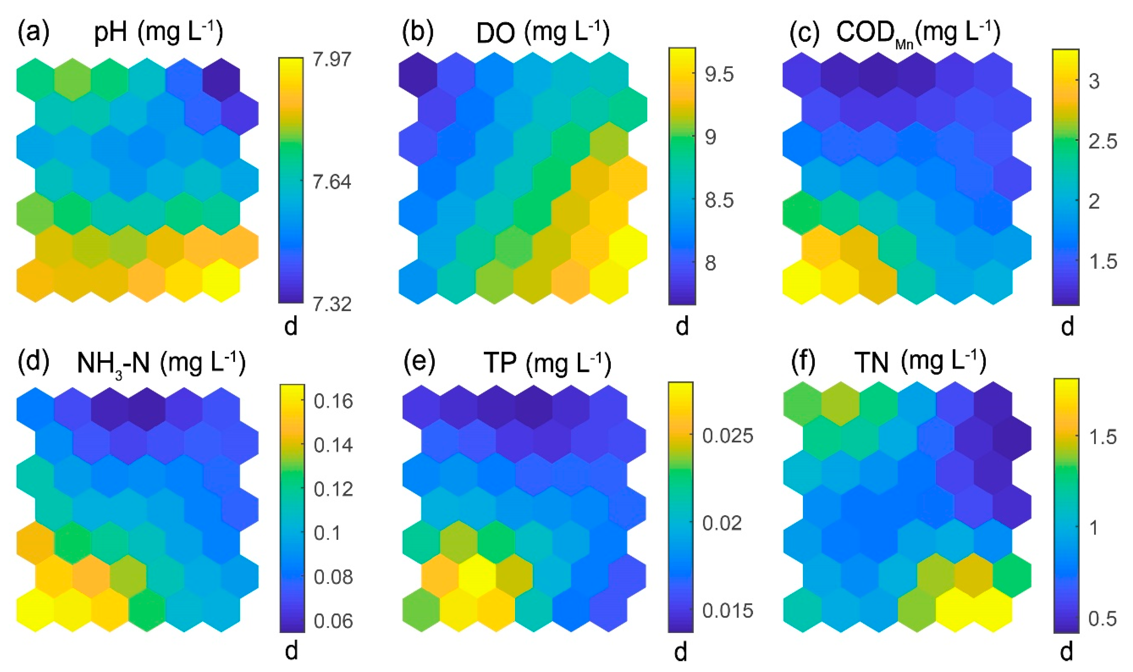
The results from SOM training (TE = 0.033, QE = 0.470) showed that the CODMn, NH3-N, and TP concentrations had similar spatial patterns, with the lowest values at the top-right and the highest values at the bottom-left part of the SOM plane (Figure 2c–e). The pH value and TN concentration differed from other parameters in the SOM plane (Figure 2a,f), showing that neither of them varied with sampling sites simultaneously. The results came out the same in the spatial distribution of water quality concentrations in the study region (Figure S2). These results indicated that the characteristics of sampling sites (e.g., elevation) might influence the water quality.
We then analyzed the relationship between the elevation and water quality of the 61 sampling sites during normal, flood, and low periods in our study area by linear regression (Figure S3). The results indicated that the elevation of reservoirs was significant negatively correlated with the CODMn concentration during normal and low periods (Figure S3). Meanwhile, the elevation of sampling sites was also significant negatively correlated with the TN concentration during all three periods (Figure S3). These results indicated that both seasonal period and elevation could influence the water quality measurements of reservoirs.
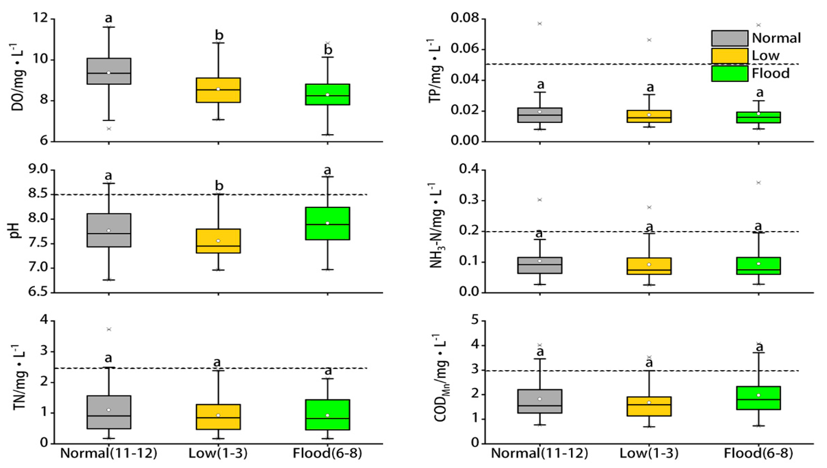
As indicated in Figure 3, the DO concentration of the reservoirs was significantly higher (p < 0.05) during the normal period (median = 9.35 mg L−1) than during the low (median = 8.53 mg L−1) and flood periods (median = 8.25 mg L−1), and the pH value was significantly higher (p < 0.05) during the normal (median = 7.71) and flood periods (median = 7.89) than during the low period (median = 7.45). Water quality was poor during the flood period as indicated by the pH and DO concentration. The other physical chemistry properties did not significantly differ among periods (Figure 3).
As indicated in Figure 4, the TN concentration and pH value were significantly higher (p < 0.05) in plain reservoirs (medianpH = 7.73; medianTN = 0.88 mg L−1) than in mountain reservoirs (medianpH = 7.39; medianTN = 0.42 mg L−1). The concentrations of CODMn (median = 1.76 mg L−1), NH3-N (median = 0.085 mg L−1), and TP (median = 0.016 mg L−1) tended to be higher and the DO (median = 8.71 mg L−1) concentration tended to be lower in the plain reservoirs, but the differences were not statistically significant (p > 0.05).

3.2. Land Use Types as Affected by Elevation and Scale

As indicated in Figure 5, the proportion of forest was higher in mountain reservoirs than in plain reservoirs, but the opposite was true for the proportions of construction land, grassland, and cropland. This indicated that reservoirs were more affected by human activity at lower elevations. Regarding scale, the proportion of construction land increased, especially for plain reservoirs, as the scale (the area under consideration) increased.

3.3. Effects of Land Use Proportions and LUI on Water Quality

We determined whether water quality properties were correlated with land use proportions and LUI as a function of elevation and scale (see Figure 5). As shown in Figure 6, a Spearman correlation heatmap indicated that LUI and the proportion of construction land had a positive correlation with the concentrations of CODMn and NH3-N (n = 61, p < 0.05). The proportion of construction land was also positively correlated with the concentrations of TP and TN and negatively correlated with the DO concentration (n = 61, p < 0.05). The proportion of forest and the proportion of grassland were negatively correlated with concentrations of CODMn, NH3-N, and TN (n = 61, p < 0.05). The proportion of cropland was negatively correlated with the CODMn concentration (Spearman’s correlation coefficient = 0.26, n = 61, p < 0.05) and not correlated with any of the other water quality properties.
Regarding scale, correlations between water quality properties and land use proportion and LUI tended to be stronger with buffers >500 m (Figure 6). The correlation between LUI (e.g., Spearman’s correlation coefficientCOD = 0.53, n = 61, p < 0.01) and the proportion of construction land (e.g., Spearman’s correlation coefficientCOD = 0.47, n = 61, p < 0.01) was stronger in the1500 m buffer than in the catchments. In the heatmap, two clusters were evident: one cluster included grassland and forest proportions, and the other included cropland proportion, construction land proportion, and LUI.
Because water quality properties differed among periods, we also calculated the Spearman’s correlation between water quality and land use proportions and LUI during the normal, low, and flood periods (Figures S4–S6). During normal and flood periods, the proportion of grassland was negatively correlated with the concentrations of CODMn, NH3-N, TN, and TP (n = 61, p < 0.05), which suggested that grassland helped to purify the water during these periods. The correlation between land use proportions and water quality properties also differed between reservoirs in mountains vs. plains (Table 1). In the 100 m and 200 m buffers of reservoirs in mountainous regions, cropland proportion was positively correlated with NH3-N concentration (n = 61, p < 0.05). In reservoirs on plains, cropland proportion was not correlated (p > 0.05) with any water quality properties, and correlations between land use proportions and water quality properties were strongest for construction land.

3.4. Effects of Land Use Configuration on Water Quality

Land use configuration (as indicated by landscape pattern indices) was another significant indicator affecting water quality (Figure 7 and Table S1). In descending order of explained variance as indicated by RDA, the percent of landscape (PLAND) for construction land was positively correlated with pH and concentrations of CODMn, NH3-N, TP, and TN in the 1500 m buffer during the low period (p = 0.002, variance = 15.1%) and during the total period (p = 0.01, variance = 11.5%) (Figure 7j,l; Table S1). In addition, the largest patch index (LPI) was negatively correlated with the concentrations of CODMn, NH3-N, and TP and was positively correlated with DO and TN concentrations at the catchment scale over the entire year (p = 0.006, variance = 11.2%) (Figure 7p and Table S1). For forest, the cohesion index (COHE) was positively correlated with CODMn, NH3-N, and TP concentrations and negatively correlated with the TN and DO concentrations (p = 0.008, variance = 10.5%) (Figure 7g and Table S1). In descending order of total explained variance, RDA further showed that for the 1500 m buffer a high proportion of construction land was found, and the influence of land use configuration on water parameters was strongest during the total period (33.0%), flood period (28.4%), and normal period (30.5%) (Table S1) compared to the other buffer scales studied. During the low period, total variance was higher with the 500 m buffer scale than with other scales (25.9%) (Table S1).

4. Discussion

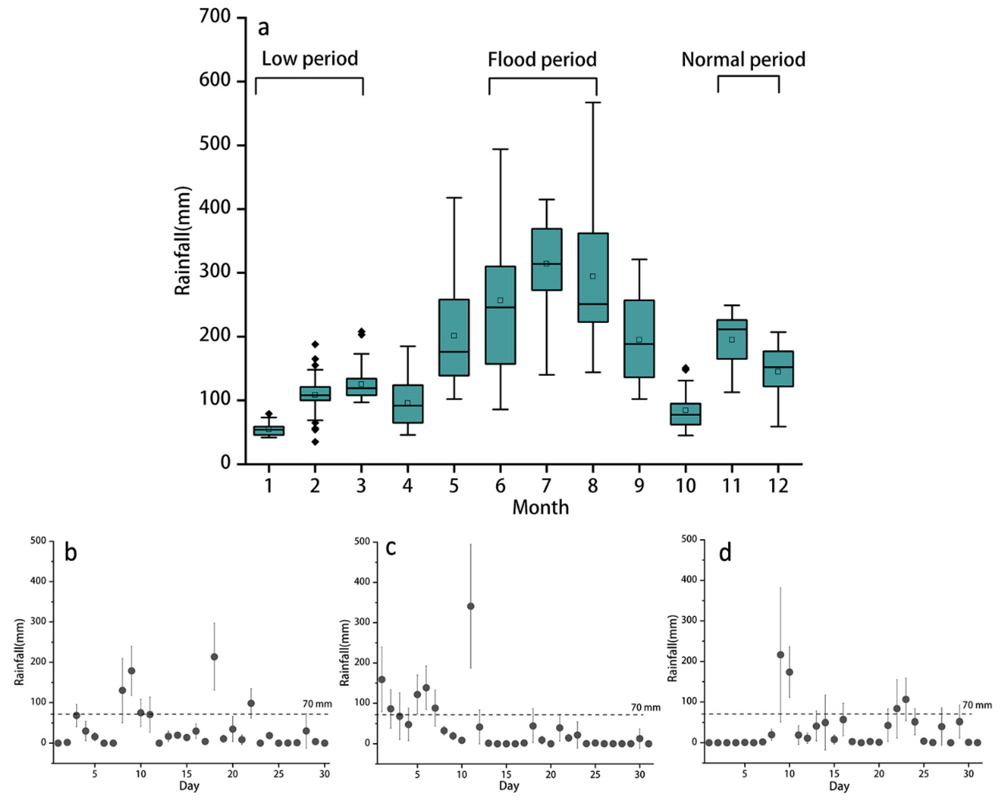
This research documented a significant seasonal change in the water quality of reservoirs in Zhejiang Province, eastern China. The pH values and DO concentrations indicated that water quality in reservoirs was poorer during the flood period, which usually occurs in summer (Figure 3 and Figure 8). Many studies have shown that water quality improves during flood periods because of the “dilution effect”, i.e., because the increased water flow reduces the concentration of pollutants [35]. Other studies, however, have reported that water quality is better during low periods than flood periods because low water levels and slow flow rates will increase the breakdown of pollutants and their removal by sedimentation [36]. Although we arrived at the same conclusion as the latter, the reasons motivating the conclusion are different. On one hand, the concentration of point-source pollutants may decrease because of the dilution effect during flood periods, while those from non-point sources should have the opposite tendency [37]. In the flood period of the current study (Figure 8a), pH was high (Figure 3) due to the absence of rainstorms (most of the daily accumulated rainfall within 12 h was below 70mm) (Figure 8b–d), which reduced the potential for a dilution effect. On the other hand, the high pH in the reservoirs might be explained by the water levels in the reservoirs, which were highest during the low period (in winter) and lowest during the flood period (in summer) [38]. During flood periods, dams significantly intercept the natural transfer of water to reservoirs [39]. Because water flows slowly through reservoirs, the retention time of pollutants in freshwater ecosystems is prolonged [40].
Water quality also differed with elevation and topography (i.e., mountains vs. plains) in our study. The elevation of reservoirs was significant negatively correlated with the CODMn and TN concentrations of reservoirs (Figure S3). The pH values and TN concentrations were significantly higher in plain reservoirs than in mountain reservoirs (Figure 4). These spatial differences may be explained by land use patterns (Table 1). The effects of human land use are often superimposed on the underlying gradients of other characteristics such as parent material, soil type, and natural topography [41], and urbanization mainly occurs in the lowlands, i.e., on plains [42]. Urban sprawl has changed adjacent stream channels, which increases the probability of non-point-source pollution [43]. In other studies, residential and commercial areas led to the accumulation of N concentration in reservoirs [14], and pollutants might support microbial activities that increase DO consumption [44]. Our results also showed that the proportion of construction land was higher near reservoirs on the plains than in the mountains and that the proportion increased as the scale increased, i.e., as the buffer area increased (Figure 5). Most reservoirs collect rainwater in catchment areas that are far away from urban areas and towns.
In this study, the correlations between water quality and land use proportions were stronger when a buffer distance surrounding the reservoirs exceeding 500 m was considered (Figure 6). The latter finding was consistent with the RDA results investigating the relationships between land use configuration and water quality (Figure 7 and Table S1) which indicated that the land use metrics could be stronger predictors of water quality at larger scales than at smaller scales. In addition to being a strong predictor of water quality during the low period, land use configuration had the strongest effect when the buffer distance was 1500 m, which included a higher proportion of construction land (Table S1). Several reports have indicated that among the factors affecting stream water quality, the presence of a 100 m wide riparian zone was the most important [25,45]. Although the local scale should have a large effect on water quality because factors at this scale function as pollutant filters [21], larger scales may have had a significant effect on water quality in the current study due to dispersal along and outside of the river network. The correlation between LUI and the construction land proportion was stronger at the 1500 m buffer scale than at the catchment scale (Figure 6), which is consistent with previous reports that the surrounding buffer is a better predictor of water quality than the entire catchment [12,46]. These results suggest that informed land use planning at a scale of 1500 m could improve the water quality in reservoirs.
There were no significant correlations between cropland proportion and water quality properties except for the CODMn concentration during the whole period. Despite the high proportion of cropland surrounding reservoirs (Figure 5), use of fertilizers was regulated by aquatic ecological red lines [47]. Although our results indicated that water quality was more affected by factors at larger scales, the local effects of the interface (water level fluctuation zone) on water quality in reservoirs should not be ignored [48]. The water level fluctuation zone is located at the aquatic–terrestrial interface, an interface that affects nutrient content and its spatial–temporal distribution by regulating the biological and non-biological processes between the freshwater and terrestrial ecosystems [49]. Land use and land cover generally have a mechanical influence on the aquatic–terrestrial interface’s habitat structure and chemical make-up, and these changes are associated with management activities. Ensuring the security of freshwater ecosystems without damaging the structure and function of the water level fluctuation zone is an important challenge.
Our results illustrated that the proportion of forest and the proportion of grassland were negatively correlated with concentrations of CODMn, NH3-N, and TN (n = 61, p < 0.05) (Figure 5). This demonstrated that forestland and grassland acted as a “sink” for potential pollutants. Therefore, for the forestland-dominated areas surrounding the reservoirs, the government should promote the construction of public welfare forests, focus on strengthening the construction of afforestation, and strengthen the protection of natural forest resources [31]. Although there were no significant correlations between cropland proportion and water quality properties (Figure 5), the policy-makers also should promote the cultivation of green manure by rotation and encourage the use of organic fertilizers outside the “ecological red line”. Our results indicated that both the proportion and the configuration of construction land can influence the water quality of reservoirs at local and watershed scales (Figure 5 and Figure 7). It is urgent to control the area of construction land and reasonably lay out the configuration of the urban area. Moreover, the local industry which produces industrial point-source pollution should limit its sewage discharge concentration, especially for the CODMn and NH3-N concentrations.
Although reservoirs differ from rivers and streams in that they are often located far from urban areas, we should not ignore large-scale land use planning, especially in a developed area like Zhejiang Province where the urbanization rate was 65.8% in 2015 (http://www.stats.gov.cn/). Our results revealed that land use planning of the interface at different scales should be adapted to local conditions and that human urban development on larger scales (1500 m from the reservoir) should be reduced. For reservoirs located in the hilly areas of South China, policy-makers should also take into account the topographic characteristics of reservoirs and seasonal differences.

5. Conclusions

Our findings revealed that the elevation of sampling sites influenced the water quality throughout the different seasons. The quality of water in reservoirs was poorer during flood periods than in other periods and was poorer for reservoirs located on plains versus in the mountains. These poor water conditions could be explained by the absence of rainstorms during the flood period in 2015–2016 (which prevented the “dilution effect”), the regulation of reservoir water levels (such that they are lowest during flood periods), and the high proportion of construction land on the plain. The LUI and the proportions of construction land were negatively correlated with CODMn and NH3-N concentrations, and RDA showed that the PLAND of construction land was positively correlated with CODMn, NH3-N, TP, and TN concentrations. During the normal period, the forest cohesion index (COHE) was the main land use metric influencing water quality and was negatively associated with the TN concentration and pH value. The total explained variance in water quality was higher with a 1500 m buffer scale than with smaller scales, indicating that management ensuring water safety should be carried out at this scale.
In previous studies, researchers only used correlation analysis or linear regression to investigate the effects of LULC on water quality. Because of the spatial–temporal variability, our research used SOM training to improve the methods to explore the spatial–temporal pattern of the water quality parameters. Our study also focused attention on reservoirs which are usually overlooked but which have played an important role in providing drinking water for human beings. Moreover, we focused on the interfaces of reservoirs that are most impacted by anthropogenic activities. Because of the particularity of reservoirs, the government should attach more importance to the seasonal variability of the water quality. The results indicated that 1500 m buffer scale could be the most applicable scale for policy-makers to manage an optimal land use pattern. However, the local effects of the interface (water level fluctuation zone) on the water quality in reservoirs should not be ignored. The stakeholders, especially for the residents, should strengthen the awareness of forest and grassland protection and observe the ecological red line policy. Moreover, the local industry which produces industrial point-source pollution should limit its sewage discharge concentration, especially for the CODMn and NH3-N concentrations. As the public pays more attention to water quality, decision-makers need more information about the value of water quality. Thus, it will also be significant to mainstream water-quality-related ecosystem goods and services into decision-making and explore the effects of LULC on these ecosystem services in our future work.

Supplementary Materials

The following are available online at https://www.mdpi.com/2071-1050/11/18/4860/s1, Table S1: The RDA results explained by explanatory variables; Figure S1: Land use types of study area; Figure S2: Spatial distribution of water quality; Figure S3: Linear relationship between elevation and water quality; Figure S4: Correlation heatmap in the normal period; Figure S5: Correlation heatmap in the low period; Figure S6: Correlation heatmap in the flood period.

Author Contributions

Conceptualization, L.D.; Methodology, L.D.; Software, L.D.; Formal Analysis, L.D. and Q.L.; Data Curation, L.D. and J.W.; Writing—Original Draft Preparation, L.D.; Writing—Review and Editing, L.D. and X.C.; Funding Acquisition, C.X. and J.T.

Funding

This work was supported by the National Key Research and Development Program of China (2016YFC0502703) and the National Natural Science Foundation of China (31570411).

Conflicts of Interest

The authors declare no conflict of interest.

References

  1. Wetzel, R.G. Limnology, Lake and River Ecosystems; Academic Press: Cambridge, MA, USA, 2001. [Google Scholar]
  2. World Resources Institute. Millennium Ecosystem Assessment. In Ecosystems and Human Well-Being, Wetlands and Water Synthesis; World Resources Institute: Washington, DC, USA, 2005. [Google Scholar]
  3. Keeler, B.L.; Polasky, S.; Brauman, K.A.; Johnson, K.A.; Finlay, J.C.; O’Neill, A.; Kovacs, K.; Dalzell, B. Linking water quality and well-being for improved assessment and valuation of ecosystem services. Proc. Natl. Acad. Sci. USA 2012, 109, 18619–18624. [Google Scholar] [CrossRef] [Green Version]
  4. Akasaka, M.; Takamura, N.; Mitsuhashi, H.; Kadono, Y. Effects of land use on aquatic macrophyte diversity and water quality of ponds. Freshw. Biol. 2010, 55, 909–922. [Google Scholar] [CrossRef]
  5. da Silva, V.D.R.; Silva, M.T.; Singh, V.P.; de Souza, E.P.; Braga, C.C.; de Holanda, R.M.; Almeida, R.S.R.; de Sousa, F.D.S.; Braga, A.C.R. Simulation of stream flow and hydrological response to land-cover changes in a tropical river basin. Catena 2018, 162, 166–176. [Google Scholar] [CrossRef]
  6. Luo, K.; Hu, X.B.; He, Q. Impacts of rapid urbanization on the water quality and macroinvertebrate communities of streams, a case study in Liangjiang New Area, China. Sci. Total Environ. 2018, 621, 1601–1614. [Google Scholar] [CrossRef]
  7. Carpenter, S.R.; Stanley, E.H.; Vander Zanden, M.J. State of the world’s freshwater ecosystems, physical, chemical, and biological changes. Annu. Rev. Environ. Resour. 2011, 36, 75–99. [Google Scholar] [CrossRef]
  8. Tegos, A.; Schlüter, W.; Gibbons, N.; Katselis, Y.; Efstratiadis, A. Assessment of environmental flows from complexity to parsimony—Lessons from lesotho. Water 2018, 10, 1293. [Google Scholar] [CrossRef]
  9. Carey, R.O.; Migliaccio, K.W.; Li, Y.C.; Schaffer, B.; Kiker, G.A.; Brown, M.T. Land use disturbance indicators and water quality variability in the Biscayne Bay Watershed, Florida. Ecol. Indic. 2011, 11, 1093–1104. [Google Scholar] [CrossRef]
  10. Chen, Q.; Mei, K.; Dahlgren, R.A.; Wang, T.; Gong, J.; Zhang, M.H. Impacts of land use and population density on seasonal surface water quality using a modified geographically weighted regression. Sci. Total Environ. 2016, 572, 450–466. [Google Scholar] [CrossRef] [Green Version]
  11. Liu, J.; Shen, Z.Y.; Chen, L. Assessing how spatial variations of land use pattern affect water quality across a typical urbanized watershed in Beijing, China. Landsc. Urban. Plan. 2018, 176, 51–63. [Google Scholar] [CrossRef]
  12. Shi, P.; Zhang, Y.; Li, Z.; Li, P.; Xu, G. Influence of land use and land cover patterns on seasonal water quality at multi-spatial scales. Catena 2017, 151, 182–190. [Google Scholar] [CrossRef]
  13. Yu, S.; Xu, Z.X.; Wu, W.; Zuo, D.P. Effect of land use types on stream water quality under seasonal variation and topographic characteristics in the Wei River basin, China. Ecol. Indic. 2016, 60, 202–212. [Google Scholar] [CrossRef]
  14. de Mello, K.; Valente, R.A.; Randhir, T.O.; dos Santos, A.C.A.; Vettorazzi, C.A. Effects of land use and land cover on water quality of low-order streams in Southeastern Brazil, watershed versus riparian zone. Catena 2018, 167, 130–138. [Google Scholar] [CrossRef]
  15. Bremigan, M.T.; Soranno, P.A.; González, M.J.; Bunnell, D.B.; Arend, K.K.; Renwick, W.H.; Stein, R.A.; Vanni, M.J. Hydrogeomorphic features mediate the effects of land use/cover on reservoir productivity and food webs. Limnol. Oceanogr. 2008, 54, 1420–1433. [Google Scholar] [CrossRef]
  16. Park, Y.S.; Kwon, Y.S.; Hwang, S.J.; Park, S. Characterizing effects of landscape and morphometric factors on water quality of reservoirs using a self-organizing map. Environ. Modell. Softw. 2014, 55, 214–221. [Google Scholar] [CrossRef]
  17. Earthscan. WCD World Commission on Dams. In Dams and Development, a Framework for Decision Making; Earthscan: London, UK, 2000. [Google Scholar]
  18. Koutsoyiannis, D. Scale of water resources development and sustainability: Small is beautiful, large is great. Hydrol. Sci. J. 2011, 56, 553–575. [Google Scholar] [CrossRef]
  19. Sargentis, G.; Ioannidis, R.; Karakatsanis, G.; Sigourou, S.; Lagaros, N.D.; Koutsoyiannis, D. The development of the athens water supply system and inferences for optimizing the scale of water infrastructures. Sustainability 2019, 11, 2657. [Google Scholar] [CrossRef]
  20. Naiman, R.J.; Décamps, H. The Ecology of Interfaces: Riparian Zones. Annu. Rev. Ecol. Syst. 1997, 28, 621–658. [Google Scholar] [CrossRef] [Green Version]
  21. Kuglerová, L.; Dynesius, M.; Laudon, H.; Jansson, R. Relationships between plant assemblages and water flow across a boreal forest landscape, a comparison of liverworts, mosses, and vascular plants. Ecosystems 2016, 19, 170–184. [Google Scholar] [CrossRef]
  22. Groffman, P.M.; Bain, D.J.; Band, L.E.; Belt, K.T.; Brush, G.S.; Grove, J.M.; Pouyat, R.V.; Yesilonis, I.C.; Zipperer, W.C. Down by the riverside, urban riparian ecology. Front. Ecol. Environ. 2003, 1, 315–321. [Google Scholar] [CrossRef]
  23. Pratt, B.; Chang, H. Effects of land cover, topography, and built structure on seasonal water quality at multiple spatial scales. J. Hazard. Mater. 2012, 209, 48–58. [Google Scholar] [CrossRef]
  24. Ding, J.; Jiang, Y.; Liu, Q.; Hou, Z.; Liao, J.; Fu, L.; Peng, Q. Influences of the land use pattern on water quality in low-order streams of the Dongjiang River basin, China, a multi-scale analysis. Sci. Total Environ. 2016, 551, 205–216. [Google Scholar] [CrossRef]
  25. Zhang, J.; Li, S.Y.; Dong, R.Z.; Jiang, C.S.; Ni, M.F. Influences of land use metrics at multi-spatial scales on seasonal water quality, a case study of river systems in the Three Gorges Reservoir Area, China. J. Clean. Prod. 2019, 206, 76–85. [Google Scholar] [CrossRef]
  26. Li, S.; Xia, X.; Tan, X.; Zhang, Q. Effects of catchment and riparian landscape setting on water chemistry and seasonal evolution of water quality in the upper Han River basin, China. PLoS ONE 2013, 8, e53163. [Google Scholar] [CrossRef]
  27. Wu, J.G. Effects of changing scale on landscape pattern analysis, scaling relations. Landsc. Ecol. 2004, 19, 125–138. [Google Scholar] [CrossRef]
  28. Lee, S.W.; Hwang, S.J.; Lee, S.B.; Hwang, H.S.; Sung, H.C. Landscape ecological approach to the relationships of land use patterns in watersheds to water quality characteristics. Landsc. Urban. Plan. 2009, 92, 80–89. [Google Scholar] [CrossRef]
  29. Marrero, H.J.; Torretta, J.P.; Medan, D. Effect of land use intensification on specialization in plant-foral visitor interaction networks in the Pampas of Argentina. Agric. Ecosyst. Environ. 2014, 188, 63–71. [Google Scholar] [CrossRef]
  30. Wu, J.L.; Zeng, H.A.; Yu, H.; Ma, L.; Xu, L.S.; Qin, B.Q. Water and Sediment Quality in Lakes along the Middle and Lower Reaches of the Yangtze River, China. Water Resour. Manag. 2012, 26, 3601–3618. [Google Scholar] [CrossRef]
  31. Ding, L.L.; Wang, Q.; Chen, X.; Tang, J.J. The responses of ecosystem services to land-use change in Dianshan Lake area from 1984 to 2014. Acta Ecologica Sinica 2019, 39, 2973–2985. (In Chinese) [Google Scholar]
  32. Liu, F.; Yan, H.M.; Liu, J.Y.; Xiao, X.M.; Qin, Y.W. Spatial pattern of land use intensity in China in 2000. Acta. Geogr. Sin. 2016, 71, 1130–1143, (In Chinese with English abstract). [Google Scholar] [CrossRef]
  33. Kohonen, T. Self-Organizing Maps; Springer: Berlin/Heidelberg, Germany, 2001. [Google Scholar]
  34. Vesanto, J.; Himberg, J.; Alhoniemi, E.; Parhankangas, J. SOM toolbox for Matlab 5. In Technical Report A57; Neural Networks Research Centre, Helsinki University of Technology: Helsinki, Finland, 2007. [Google Scholar]
  35. Long, D.T.; Pearson, A.L.; Voice, T.C.; Polanco-Rodriguez, A.G.; Sanchez-Rodriguez, E.C.; Xagoraraki, I.; Concha-Valdez, F.G.; Puc-Franco, M.; Lopez-Cetz, R.; Rzotkiewicz, A.T. Influence of rainy season and land use on drinking water quality in a karst landscape, State of Yucatán, Mexico. Appl. Geochem. 2018, 98, 265–277. [Google Scholar] [CrossRef]
  36. Sunohara, M.D.; Gottschall, N.; Craiovan, E.; Wilkes, G.; Topp, E.; Frey, S.K.; Lapen, D.R. Controlling tile drainage during the growing season in eastern Canada to reduce nitrogen, phosphorus, and bacteria loading to surface water. Agric. Water Manag. 2016, 178, 159–170. [Google Scholar] [CrossRef]
  37. Wang, X.L.; Zhang, L.; Zhao, Z.H.; Cai, Y.J. Heavy metal pollution in reservoirs in the hilly area of southern China, distribution, source apportionment and health risk assessment. Sci. Total Environ. 2018, 634, 158–169. [Google Scholar] [CrossRef]
  38. Zhu, H.; Bing, H.J.; Wu, Y.H.; Zhou, J.; Sun, H.Y.; Wang, J.P.; Wang, X.X. The spatial and vertical distribution of heavy metal contamination in sediments of the Three Gorges Reservoir determined by anti-seasonal flow regulation. Sci. Total Environ. 2019, 664, 79–88. [Google Scholar] [CrossRef]
  39. Yang, H.F.; Yang, S.L.; Xu, K.H.; Milliman, J.D.; Wang, H.; Yang, Z.; Chen, Z.; Zhang, C.Y. Human impacts on sediment in the Yangtze River, a review and new perspectives. Glob. Planet. Chang. 2018, 162, 8–17. [Google Scholar] [CrossRef]
  40. Tong, Y.D.; Li, J.Q.; Qi, M.; Zhang, X.Y.; Wang, M.Z.; Liu, X.Y.; Zhang, W.; Wang, X.J.; Lu, Y.R.; Lin, Y. Impacts of water residence time on nitrogen budget of lakes and reservoirs. Sci. Total Environ. 2019, 646, 75–83. [Google Scholar] [CrossRef]
  41. Allan, J.D. Landscapes and riverscapes, the influence of land use on stream ecosystems. Annu. Rev. Ecol. Evol. Syst. 2004, 35, 257–284. [Google Scholar] [CrossRef]
  42. Basnou, C.; Álvarez, E.; Bagaria, G.; Guardiola, M.; Isern, R.; Vicente, P.; Pino, J. Spatial patterns of land use changes across a Mediterranean metropolitan landscape, implications for biodiversity management. Environ. Manag. 2013, 52, 971–980. [Google Scholar] [CrossRef]
  43. Li, T.H.; Bai, F.J.; Han, P.; Zhang, Y.Y. Non-point source pollutant load variation in rapid urbanization areas by Remote Sensing, Gis and the L-THIA Model, a Case in Bao’an District, Shenzhen, China. Environ. Manag. 2016, 58, 873–888. [Google Scholar] [CrossRef]
  44. Tsegaye, T.; Sheppard, D.; Islam, K.R.; Johnson, A.; Tadesse, W.; Atalay, A.; Marzen, L. Development of chemical index as a measure of in-stream water quality in response to land-use and land cover changes. Water Air Soil Pollut. 2006, 174, 161–179. [Google Scholar] [CrossRef]
  45. Ou, Y.; Wang, X.Y.; Wang, L.X.; Rousseau, A.N. Landscape influences on water quality in riparian buffer zone of drinking water source area, Northern China. Environ. Earth. Sci. 2016, 75, 114. [Google Scholar] [CrossRef]
  46. Shen, Z.; Hou, X.; Li, W.; Aini, G.; Chen, L.; Gong, Y. Impact of landscape pattern at multiple spatial scales on water quality, a case study in a typical urbanized watershed in China. Ecol. Indic. 2015, 48, 417–427. [Google Scholar] [CrossRef]
  47. Shang, W.X.; Wang, Z.J.; Zhao, Z.N.; Qiu, B.; Zheng, Z.L. Framework and delimitation study of aquatic ecological red-line. J. Hydraul. Eng. ASCE 2016, 47, 934–941. [Google Scholar] [CrossRef]
  48. Minshall, G.W.; Rugenski, A. Methods in Stream Ecology; Academic Press: Burlington, MA, USA, 2007. [Google Scholar]
  49. Zhang, H.J.; Wang, R.Q.; Wang, X.; Du, N.; Ge, X.L.; Du, Y.D.; Liu, J. Recurrent water level fluctuation alleviates the effects of submergence stress on the invasive riparian plant Alternanthera philoxeroides. PLoS ONE 2015, 10, e0129549. [Google Scholar] [CrossRef]
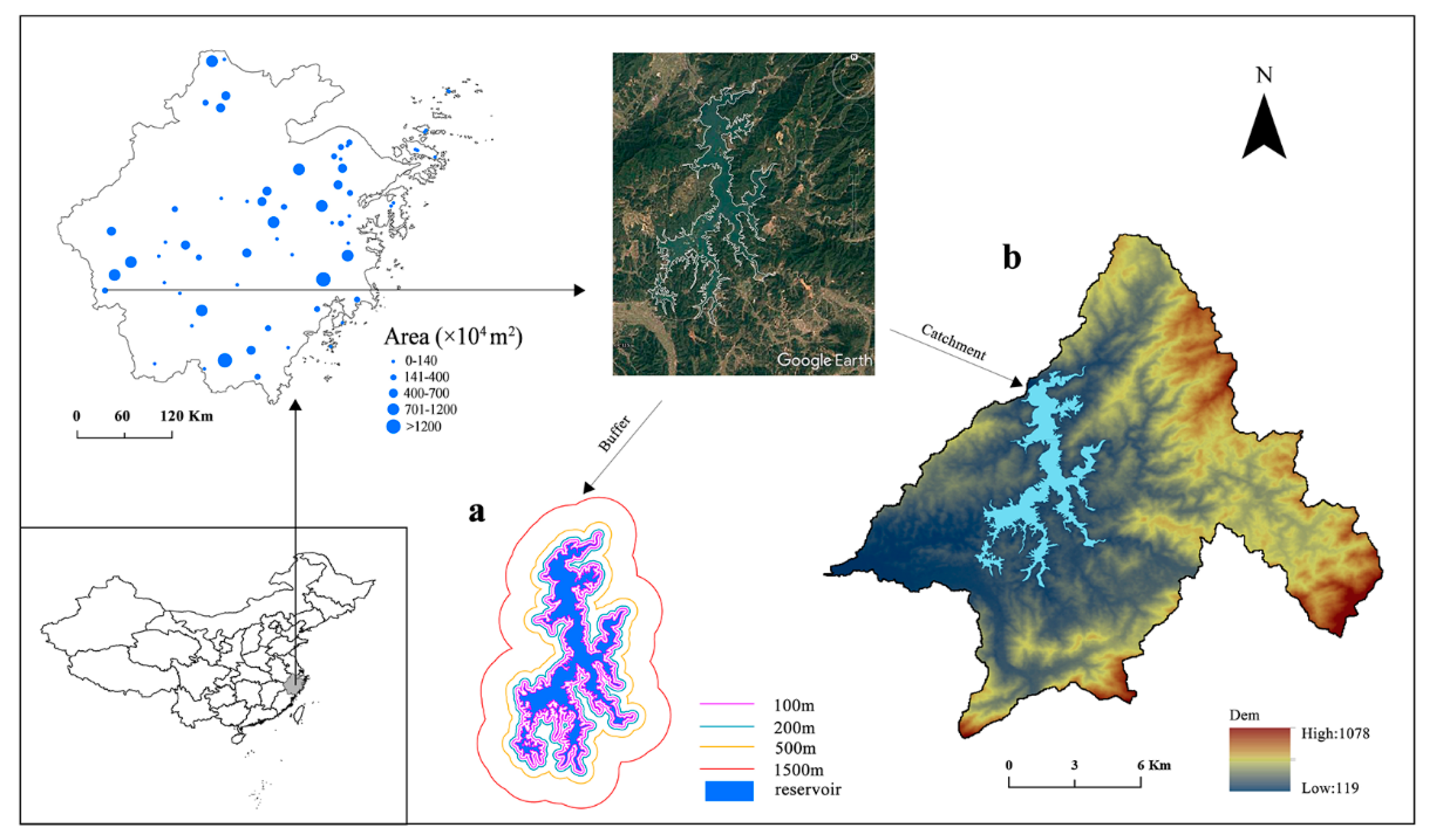
Figure 1. The locations and areas of the 61 reservoirs in Zhejiang Province. Five spatial scales are also designated: areas within 100 m, 200 m, 500 m, and 1500 m of the reservoir (referred to as buffer scales) (a) and the entire catchment (b).
Sustainability 11 04860 g001
Figure 2. The trained self-organizing map (SOM) plane of visualization of each variable. The variables included the pH value (pH), dissolved oxygen (DO), chemical oxygen demand (CODMn), total phosphorus (TP), total nitrogen (TN), and ammonia nitrogen (NH3-N). Note: “d” under the legend denotes the denormalization of the SOM data, while yellow and blue units represent high and low levels, respectively, of each environmental variable.
Sustainability 11 04860 g002
Figure 3. Physical chemistry properties of the reservoirs during different periods of the year (normal, low, and flood, which refer to water levels in rivers and streams rather than in reservoirs). The points and solid lines within each box represent the mean and median values, respectively, and the boxes represent the 25th to 75th percentiles of the distribution. In each box, values indicated by different letters are significantly different at p < 0.05. Values below the dotted line indicate meeting the standards of water quality except for dissolved oxygen (values over 5 mg L−1 meant meeting the standards).
Sustainability 11 04860 g003
Figure 4. Physical chemistry properties of the reservoirs for different reservoir elevations (mountain vs. plain). The points and solid lines within each box represent the mean and median values, respectively, and the boxes represent the 25th to 75th percentiles of the distribution. In each box, values with different letters are significantly different at p < 0.05. Values below the dotted line indicate meeting the standards of water quality except for dissolved oxygen (values over 5 mg L−1 meant meeting the standards).
Sustainability 11 04860 g004
Figure 5. The proportion of area by land use types (cropland, forestland, grassland, and construction land) for different elevations and scales. “Catchment” refers to the entire drainage basin. Values of 100, 200, 500, and 1500 m refer to the area within 100, 200, 500, and 1500 m of the reservoir, respectively. Values are means + SE.
Sustainability 11 04860 g005
Figure 6. Spearman correlation heatmap based on water quality properties, land use proportions, and land use intensity (LUI). The X and Y axes of the thermal graph are the water quality properties and land use proportions, respectively. Correlation coefficients (r values) are represented by different colors, as indicated by the scale to the right of the heatmap. * and ** indicate that means are significantly different at p < 0.05 and p < 0.01, respectively. Land use type proportions are indicated by abbreviations (for: forest; gra: grassland; cro: cropland; con: construction land). The number after the dash indicates the scale, i.e., the radius of the “buffer” area surrounding the reservoir.
Sustainability 11 04860 g006
Figure 7. Biplots of redundancy analysis (RDA) in the normal period, low period, flood period, and over the whole year. The red arrows represent the explanatory variables, and the blue arrows represent the response variables. Land use types are indicated by lower case letters in the red arrow labels (for: forest; gra: grassland; wat: waterbody; cro: cropland; con: construction land).
Sustainability 11 04860 g007
Figure 8. Monthly changes in precipitation at the 61 reservoirs during 2015–2016 (a) and daily changes in precipitation during the flood period (June (b), July (c), and August (d)). The dashed line indicates accumulated rainfall of 70 mm from 8 a.m. to 8 p.m. every day.
Sustainability 11 04860 g008
Table 1. Correlations between land use proportions (and land use intensity) and water quality properties. Correlation coefficients (and their p values in parentheses) are indicated. Values for relationships that were not statistically significant (p > 0.05) are not shown.
Land Use TypesScalepHDOCODMnNH3-NTPTN
MountainCropland100 m buffer 0.85(0.002)
200 m buffer 0.79(0.007)
GrasslandCatchment 0.70(0.025)
Construction land200 m buffer −0.70(0.024)
500 m buffer −0.81(0.005)
Land use intensity100 m buffer 0.85(0.002)
200 m buffer 0.77(0.01)
PlainGrassland100 m buffer−0.49(0.001) −0.32(0.033)
200 m buffer−0.49(0.001) −0.31(0.039)
1500 m buffer −0.34(0.024)
Catchment−0.41(0.006)−0.41(0.006)−0.32(0.036)
Forest200 m buffer−0.32(0.032)
1500 m buffer −0.44(0.003)
Catchment −0.39(0.009)−0.32(0.037)
Construction land100 m buffer −0.31(0.039) 0.32(0.035)
200 m buffer −0.32(0.037)
1500 m buffer0.34(0.024) 0.41(0.005)0.38(0.011)0.31(0.038)
Catchment0.40(0.007) 0.40(0.008)
Land use intensity200 m buffer 0.34(0.023)
500 m buffer 0.41(0.006)0.36(0.017)
1500 m buffer0.37(0.013) 0.51(0.000)0.32(0.033)
Catchment0.42(0.005) 0.39(0.008)