An Urban System Optimization Model Based on CO₂ Sequestration Index: A Big Data Analytics Approach

Abstract

Urban development in recent decades has had a significant impact on climate change. Cities have implemented traffic monitoring systems to sustain the new building code in meeting the target for environmental indicators. Timisoara is the second city in Romania and manages over 60% of the development and pollution of Timis County. The analysis of large volumes of data provided by local sensors and databases requires big data analytics. In this research, for the first time, we simultaneously developed two parallel scenario-based decision-making support models to assess a CO₂ sequestration index. The model is based on a tree inventory for traffic area and car flow using Roegenian processes with borders. The first scenario (dt1) analyzes the real O₂-pollution car flows for process streets as receivers of pollution. The second scenario (dt2) analyzes O₂-pollution flows for the same streets from the perspective of streets that garage the cars. We modeled the parallel integration of actual O₂ production and pollution flows for 160 main streets that account for over 50% of the urban mileage of Timisoara city. The carbon sequestration indexes of the streets are in the range of 0.0000043–0.437 (dt1) and 0.0000092–11.78 (dt2). The results can be used to support local decision making regarding the environment CO₂-O₂ balances by optimizing the local fiscal policies. The research could be extended to secondary streets and separately for the pollution of heating-cooling devices for residential building areas.

1. Introduction

Cities are becoming vulnerable to climate change [1]. Analytical efforts to model a city with a neutral CO₂ indicator, noticed for maintaining pollution relative to a fixed year, are expanding in Europe [2]. Two decades ago, some cities started to perform a green inventory for traffic and residential areas. The integrated inventory for over 35 characteristics of trees was done for all the street areas with a significant leaf area index (LAI) in Timisoara [3]. In the city, main streets are the highest traffic polluter [4]. In other regions of the world, researchers have analyzed and highlighted the street greenery and the capabilities of trees to produce oxygen for carbon sequestration [5,6,7,8,9].

Today, urban development benefits from the use of large-scale IT&C (Information Technology & Communication) infrastructures to investigate energy use for pollution-related and economic-social characteristics. The trend is higher as cities tend to reach the standards of a smart city with a high ecological, economic and social balance [10,11] for nano- and micro-levels (street segments and streets) for the new building code [12]. In environmental research, the use of IoT (Internet of Things) based sensor infrastructures, satellites [13], data, and information on the Internet generates large volumes of heterogeneous data by using integrated models [14]. These massive amounts of data collected from sensors or IoT infrastructures for environmental parameter monitoring contain correlations and trends that are difficult to identify without the use of artificial intelligence data analysis models. The need to model industrial, economic, and environmental data based on the new technologies such as big data (BD) and big data analytics (BDA) is outlined by various research [15,16,17,18,19].

Currently, the use of BD and BDA for recording, monitoring, and analyzing environmental parameters is an essential resource for decision-making processes in urban development policies [20].

There are many definitions of big data in the literature and practice. An illustrative definition highlights three basic features of BD: volume, velocity, and variety [21]. For environmental and socio-economic research, BD represents massive collections of unstructured, heterogeneous data on environmental parameters and indicators that are highly significant for decision making.

BDA adds value to the decision-making process [22]. It integrates data mining and machine learning methods and algorithms for descriptive and predictive BD analysis and presentation. Data mining is used for hidden patterns, correlations, or knowledge discovery in large data sets like big data environments [15,22]. Other recent research has used the deep learning approach based on statistics with trained neural networks for measuring social, environmental, and health inequalities within London [23].

Clustering, as a data mining or machine learning method, is used to discover segmentation patterns. In recent years, clustering and other data mining techniques have been successfully used in environmental and socio-economic research [24,25]. The most widely used clustering algorithm is K-means, which was developed for the first time by Lloyd in 1957 [26]. This algorithm is currently used in data mining [24,27] and involves starting with k values (random) and building clusters according to them [22]. It is an algorithm for grouping data objects based on their attributes into several clusters by minimizing the Euclidean distance between each data object from dataset and clusters centroids (mean vectors). The clusters are built iteratively. After each iteration, cluster centroids are recalculated and objects are reallocated. The iterations continue until no more object groups are possible. Thus, the K-means clustering algorithm represents a variance minimization technique.

Street and urban zones clustering according to the values of the environmental variables and the socio-economic ones represents an appropriate model of the decision-making process in urban socio-economic policies [28]. The capacity of BD for providing data and information for urban processes is based on artificial intelligence technologies (data mining and machine learning) [22,29].

Under the CO₂ pollution decreasing target, Timisoara Local Council decided to develop a traffic monitoring system [30] using the characteristics of BD to sustain the environmental policies. Among other functions, the monitoring system will contribute to “reducing travel time in the city and, implicitly, fuel consumption and emissions”. The data about car flow for three characteristics (number, speed, and weight) are currently used to optimize the traffic for main streets.

According to Skupin et al. [31], spatialization is a systematic way of transforming high-dimensional data sets into a lower-dimensional spatial representation for data visualization support, exploration, and knowledge construction. In our model, we used urban spatialization to represent the clusters.

Our research will model the traffic area using Roegenian processes with temporal and spatial borders [32] for CO₂ pollution and oxygen production on the streets. The research aims to develop two scenario-based decision support system for modeling the CO₂ sequestration index in an area with high traffic density. The results are used for system optimization based on O₂-pollution flows to support the local decision-making process regarding the environment and urban development within the new building code [12].

2. Instruments and Methods

The primary objective of this research is to create a model for the metrics of a CO₂ index based on the BDA approach. Our model develops two scenarios, based on pollution-receiver streets (in-situ-pollution by street, SPS) and pollution-donor streets (residence-car as pollution-source, RCPS).

The first scenario (dt1) models the process streets as receivers of pollution. In this case, the streets are the spatial areas where the energy used by cars will generate pollution. On the CO₂ chain from the cradle to the grave, the urban streets as Roegenian fund are the authors of “the effect” of pollution through the action processes of two main anthropomorphic agents: drivers and pedestrians. The second scenario (dt2) analyses the perspective of streets that garage the cars. Under this scenario, the streets and the owners of the cars are viewed as Roegenian funds. They are considered as the moral (real) author and the first cause of pollution.

We created a descriptive framework for the analysis of the traffic process, based on fuel use, CO₂ sequestration/pollution, and O₂ production on all of the 160 main streets.

The street areas (without residential building areas) are observed as partial Roegenian processes with spatial and temporal borders, based on the requirements of the flow-funds model [32]. We considered only the contribution of O₂ from trees in 2013 according to average daily productivity [3,13,33]. The car flows are observed for 24 h for the main intersections of streets. The starting point is the 14 h of car flows [30].

We also modeled the O₂ production for an average day of the 150-day vegetation season (15 April–15 September). The metrics are modeled starting from the figures found in [3] and [12].

In the collection and analysis process based on the two scenarios (dt1 and dt2), the collected data are structured into two categories: (1) data common to both analysis scenarios and (2) data specific to each scenario.

2.1. Data Sources

For O₂ production and car pollution flows level, the sources were [3] and [30]. For the first modeling scenario (dt1), the core data of car flows for 14 h level were collected from [30].

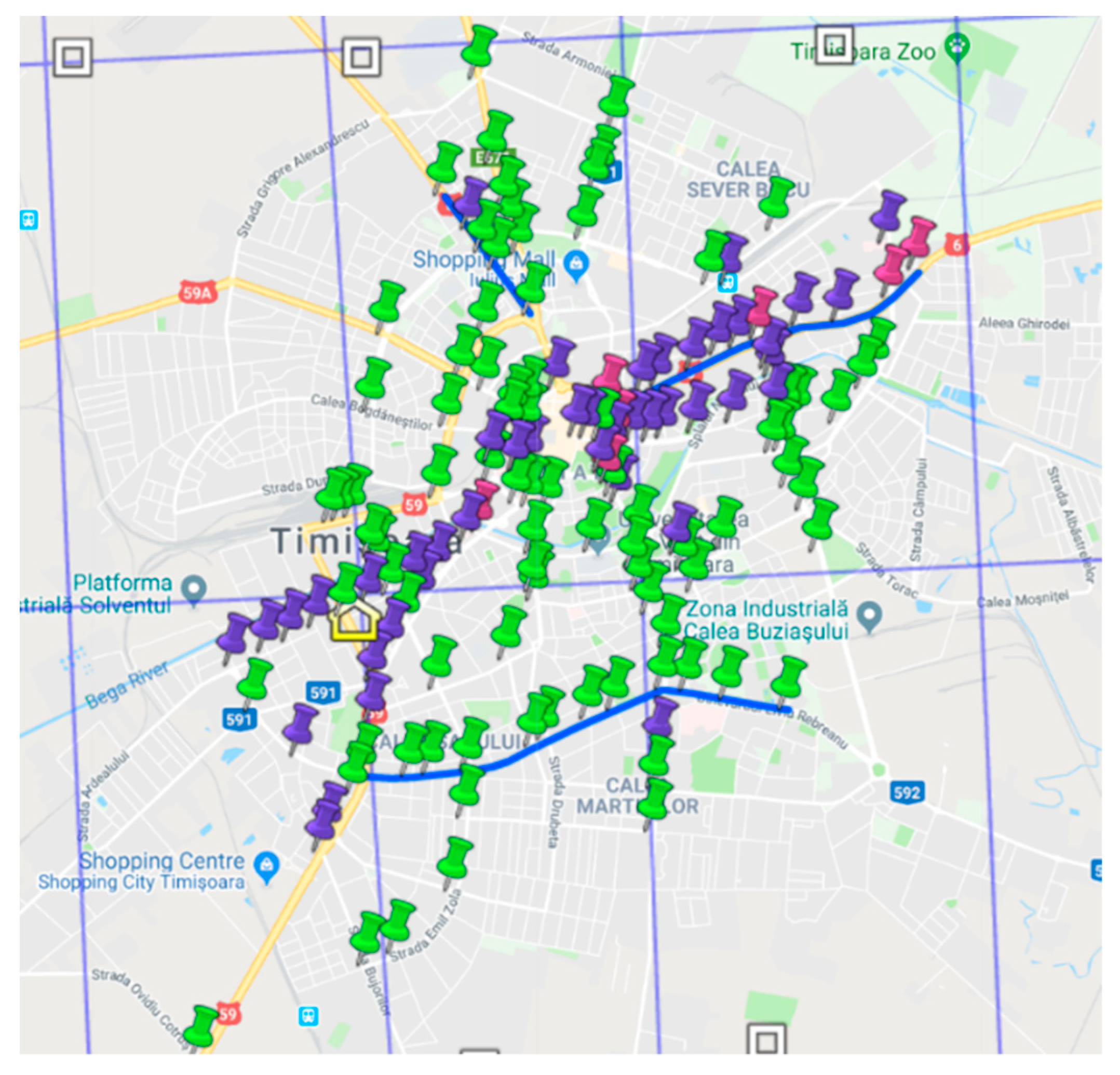
The data were integrated with the data collected from 134 sensors (Figure 1), which collect approximately 1,600,000 traffic flow records per day. These sensors are optical devices that record a signal at each car passing. These devices are located on the streets within the TCH (Timisoara City Hall) flow optimization system [30]. The data collected by the sensors were used to shift from the flow for 14 h [30] to the flow for 24 h.

For the second scenario (dt2) the data come from the statistics for population records for 2017 [12], and the average income in RON (Romanian Leu) of the households is based on statistics of the Romanian Ministry of Finance.

2.2. Variables

The common variables for the two scenarios (dt1 and dt2) are total length of the 160 streets in meters, length_meter; population on the street as number of individuals, population; the average income in RON lei of the people, income_2013; and the amount of oxygen estimated as daily productivity, O₂_d1_010 [3].

For the first scenario (dt1) we have the following specific variables: car flow in 24 h, cars_flow_24h_d1; car mileage in 24 h, mileage_24h_d1; and sequestration index in scenario dt1, index_d1def.

For the second scenario (dt2) we have the following specific variables: the number of cars parked (residing) on street i = 1, …, 160, cars_d2_2016 and sequestration index in scenario dt2, index_d2def.

Calculation of pollution

The variables of the two scenarios are modeled using the next formula system. The calculation of energy use and CO₂ was made separately for the two scenarios.

The calculation of CO₂ in the dt1 scenario was made according to Formula (1):

CO₂ = length_meter × cars_flow_24h_d1 × CO₂factorem

(1)

where length_meter represents the length of the street (meters); cars_flow_24h_d1 represents the flow of cars per 24 h on one street. The unweighted average of street segment flows for 14 h was multiplied by 1.2 times for passing to the 24-h level; CO₂factorem represents CO₂ emission factor (0.224 CO₂ kg/km). For all vehicles in 2013 in Romania, this level was 0.299 CO₂ kg per kilometer.

For the second scenario (dt2), we applied the following formula:

CO₂ = cars_d2_2016 × DM × AF × CO₂factorem

(2)

where cars_d2_2016 represents the number of cars garaged (residing) on-street i = 1, …, 160; DM is the average daily mileage of one car; AF represents the amplifying factor (

Table 1. The amplifying factor for the car density.

Differentiation Indexes	Amplifying Factor (AF)
>1.00	1.15
0.51–1.00	0.95
0.25–0.50	0.75
0.01–0.25	0.65

); CO₂factorem is the CO₂ emission factor.

The amplifying factor has four levels for the streets and is calculated according to the differentiation index for population density on the street.

The level of amplifying factor is assigned based on differentiation indexes of street density. The total mileage for Timisoara is maintained after using AF.

The differentiation index for the density of cars on the street was calculated as the ratio between the number of people resident and the street length. One level of the amplifying factor was assigned to each of the four ranges of indexes. The average mileage of 22.62 km per day per car for Timisoara was corrected with the amplifying factor based on five levels of the assigned differentiation index. The average mileage of 6786 km for one car for Timisoara was calculated for 300 days observed with significant daily flows during a year. The total mileage for the 160 streets after using the amplifying factor was calibrated using total mileage for Timisoara and Timis county [12].

The green inventory and O₂ production

We considered a 150-day vegetation period (April 15–September 15) with net O₂ productivity of 0.100 kg O₂ (LAI) per year. The productivity level is in line with Nowak et al. [33] and Running et al. [13] estimates. The O₂ intake of the green street area (grass, turf) is considered to cover pedestrian and driver’s breathing.

We built a real spatial index (ratio) for carbon sequestration, with the following formula:

spatial index for CO₂ sequestration = CO₂O₂equiv/CO₂

(3)

where CO₂ represents CO₂ emissions daily of the vehicles in Timisoara, and CO₂O2equiv represents the equivalent of CO₂ used for O₂ tree production. The indexes are calculated in both dt1 and dt2 scenarios.

Along with the two CO₂ indexes in both scenarios, we used six variables considered independent, out of which three are common. We analyzed the two scenarios separately.

2.3. Data Analysis

For the analytics modeling, we performed the following analysis: (1) descriptive statistics analysis, (2) data mining using clustering, and (3) spatialization.

(1)

In the descriptive statistics analysis, we calculated a set of statistical indicators for analyzing the data consistency of the two scenarios.

(2)

We used a K-means algorithm for clustering. This algorithm involves grouping dataset elements (variables) into k clusters by minimizing the Euclidean distance (dE) between each element and the cluster centroids (mean vectors) [34,35].

(3)

For spatialization, we represented the clusters obtained on the city map to ensure a spatial landscape for decision support.

2.4. Tools

The modeling of the descriptive data was done in R version 3.5.0 [36], both at the level of data gathering from data sources and the level of descriptive analysis and modeling of data mining through clustering.

3. Results and Discussion

In this paper, we modeled the metrics for a CO₂ sequestration index based on the BDA approach. We measured the daily flows for CO₂ vehicle emissions for all of the 160 main street areas in Timisoara, and we integrated the O₂ production of trees. The green inventory (trees) and the cars are considered as main Roegenian fund [32]. The main aim was to offer metrics to the decision-making process in the environmental area for sustaining human well-being [23].

The calculation was made for the data available in 2013 using flow modeling according to the flow-funds model requirements by considering the spatial borders of streets (without residential building areas) and temporal border by one warm season day (24 hours). The number of annual days with a significant flow is considered 300.

In the research, through the K-means algorithm, we identified the pattern of grouping streets using a predefined number of clusters. The metrics set the different levels of spatial CO₂ sequestration indices in correlation with some socio-economic variables of streets (population, income, cars).

In the dt1 scenario, the level of CO₂ sequestration index shows the capacity to retain partially the CO₂ volume emitted daily by the vehicles. The CO₂ flow of the integrated process for O₂ production and carbon sequestration is modeled at a micro-urban street level for the first time in research according to our knowledge. The complementary scenario (dt2) of carbon sequestration capability generated by cars with garage residences on each street assures the parallel observation of the primary source of pollution. The value “1” for the index means absolute neutral CO₂ (zero CO₂ emissions). In this case, we consider the zero value of CO₂ as a reference point on the time scale. The research about metrics of neutral CO₂ regularly use the level of CO₂ in 2005 as a reference point [2].

For the oceanic climate areas, the maintaining of CO₂ emissions level found in 2005 could be a prerequisite for avoiding heat islands. The higher velocity of air inside these areas can be a temporary advantage compared with some areas with a temperate continental climate. For the last areas, the relative steady-state of the CO₂ emissions level existing for 2005 seems not to be a prerequisite for avoiding the hot air on the streets or the heat islands inside urban continental climate areas [37] for a slow velocity. Under these terms, the relationship between CO₂ and O₂ production inside of continent is primarily to maintain the necessary conditions for the life of human collectives inside every small (street) residential area with no air velocity. Consequently, the new CO₂ index assessment with zero CO₂ pollution can sustain decision making for public authorities under the new climate change.

3.1. Descriptive Statistics Analysis

For the consistency of the variables for each of the scenarios, we calculated, in

Table 2. Statistical indicators for the common variables.

Indicators	Length_Meter	Population	Income_2013	O2_d1_010
nbr.val	160	160	160	160
Min	77	1	1000	0.032562507
Max	7665	4649	64,585,967	60.46602099
Range	7588	4648	64,584,967	60.43345848
Sum	187,594	125,998	1,903,359,678	1283.688954
Median	771.5	465.5	6,647,519	4.440580944
Mean	1172.4625	787.4875	11,895,997.99	8.02305596
SE.mean	93.72724876	71.64093018	1,073,529.148	0.800877753
CI.mean	185.1109613	141.4905658	2,120,216.002	1.581730529
Var	1,405,567.546	821,187.6602	1.84394 × 1014	102.624828
std.dev	1185.56634	906.1940522	13,579,188.97	10.13039131
coef.var	1.01117634	1.150740872	1.141492205	1.262659934

Note: The indicator abbreviations are according to R software notations.

, a set of statistical indicators for the variables in both scenarios.

The characteristics range is from 1–4649 times except for income, which is from 1–64586 times. The median is below the average for all the characteristics. The variation coefficient ranges below 15%, except for O₂ production, which is almost double (26%).

In

Table 3. Statistical indicators for scenario dt1.

Indicators	Cars_Flow_24h_d1	Mileage	Index_d1def
nbr.val	160	160	160
min	244.991	214,609.72	4.29 × 10−6
max	55,666.268	295,940,236.6	0.436784471
range	55,421.277	295,725,626.9	0.436780184
sum	1,917,697.147	2,759,746,683	2.934747138
median	6455.1235	4,269,557.791	0.004018895
mean	11,985.60717	17,248,416.77	0.01834217
SE.mean	992.303315	3,089,678.248	0.003377084
CI.mean	1959.795289	6,102,102.839	0.006669728
var	157,546,539	1.52738 × 1015	0.001824751
std.dev	12,551.75442	39,081,682.01	0.042717105
coef.var	1.047235592	2.265812714	2.328901451

, we present the statistical indicators for the scenario based on pollution-receiver streets (dt1).

The characteristics range by 227 times for car flow, by 1379 times for miles, and by 101,815 times for carbon sequestration index. The median is 0.247 times higher than the average for mileage and 0.22 times the index average. The variation coefficient ranges for the three variables by 1.04 to car flows and 2.33 to the sequestration index, having a value close to 2.26 for mileage.

In

Table 4. Statistical indicators for scenario dt2.

Indicators	Cars_d2_2016	Mileage_24hd2	Index_d2def
nbr.val	160	160	160
min	1	13,572	9.18 × 10−6
max	2567	55,162,263	11.78262438
range	2566	55,148,691	11.7826152
sum	61,509	1,379,919,528	22.83216356
median	231.5	4,598,646	0.005231502
mean	384.43125	8,624,497.05	0.142701022
SE.mean	35.60800805	874,191.2254	0.082186308
CI.mean	70.32568105	1,726,524.359	0.162317647
var	202,868.838	1.22274 × 1014	1.080734269
std.dev	450.4096336	11,057,741.53	1.0395837
coef.var	1.171625963	1.282131754	7.285047321

, we present the statistical indicators for the scenario based on pollution-donor streets (dt2).

The characteristics range by 2567 times for cars, by 4067 times for miles, and by 1.28 million times for carbon sequestration index. The median is about half of the mileage average and 0.036 for the index. The variation coefficient has an increasing trend in dt2, compared to dt1, for the sequestration index and a decreasing trend for mileage.

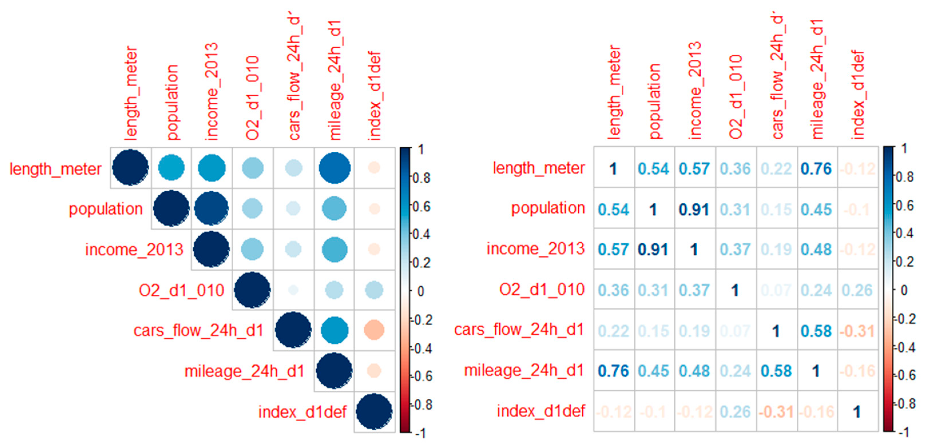
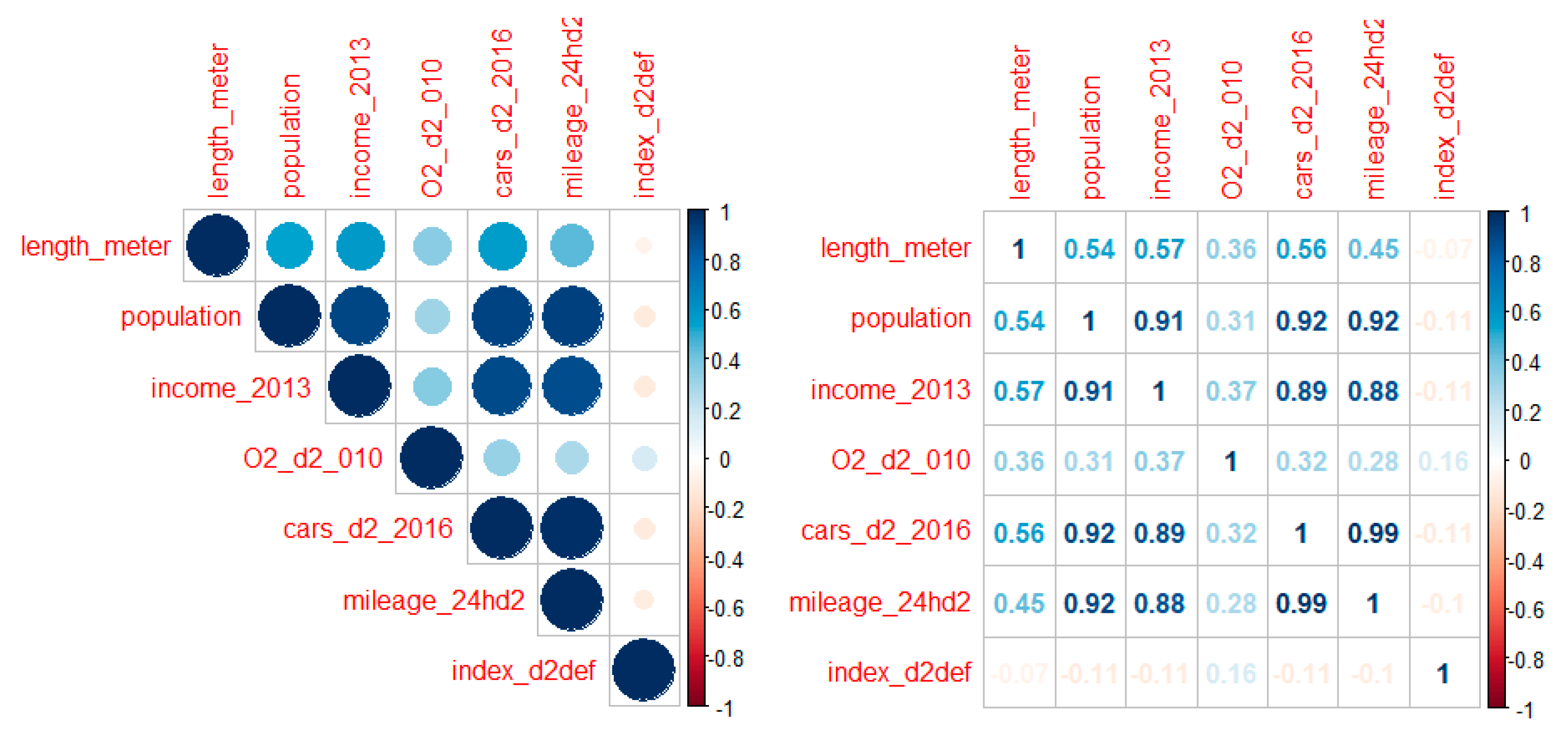
To identify the correlations between the variables, we elaborated on correlation matrices for each of the two scenarios. Within the correlation coefficient matrix, the link between variables is represented by both a numeric value and the plot bubble size.

The first result of the correlation is the correlation matrix for scenario dt1 (Figure 2).

The main positive correlation (except between common variables) is between street length and mileage by 0.76. The main negative correlation is between car flows and sequestration CO₂ index by 0.31.

The next result of the correlation analysis is the correlation matrix for the dt2 scenario (Figure 3).

The basic positive correlation is between the population and the car numbers by 0.92, with a similar correlation value of population with mileage (0.92) and income (0.91). The main negative correlation is between car flows and sequestration CO₂ index by 0.11. The correlation between car number and mileage is 0.99. The street mileage was differentiated in the analysis using the amplifying factor (AF).

3.2. Data Mining Clustering Analysis

Clustering in data mining usually serves as exploratory analysis, identifying the patterns of behavior within the dataset. Data behavior determines their segmentation (grouping) in clusters.

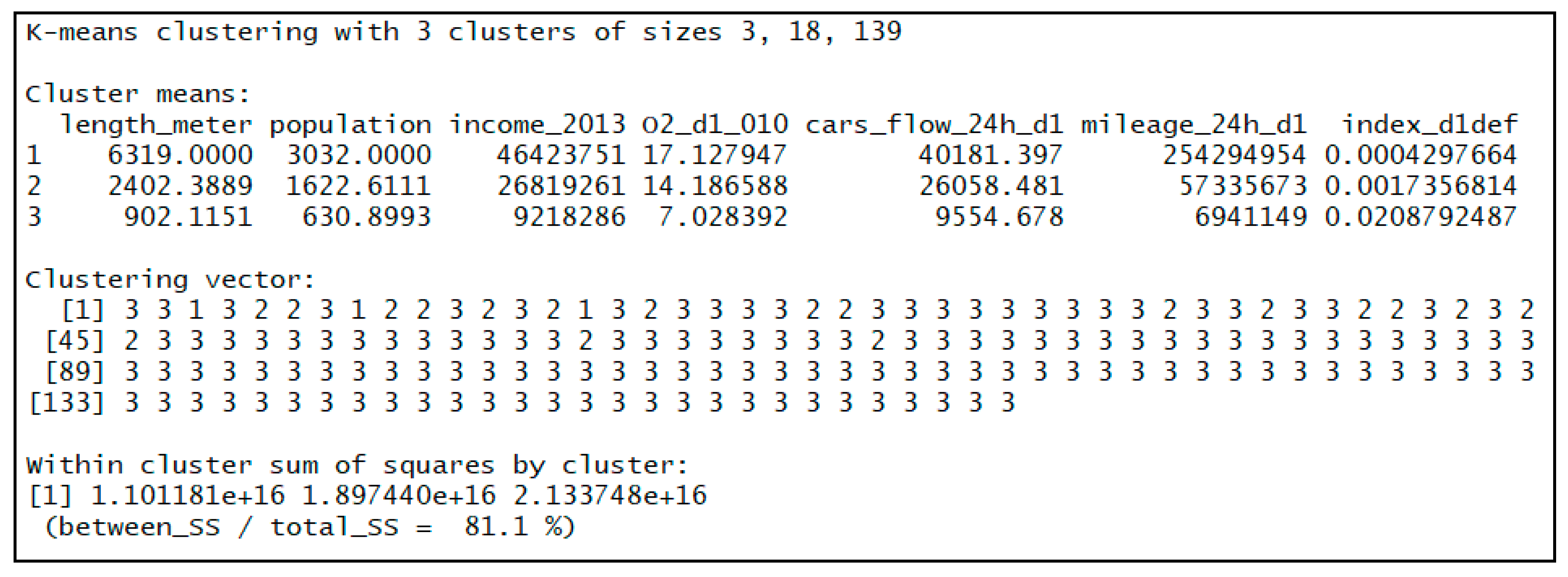
For the dt1 scenario, following data mining clustering through K-means, on a pre-defined 3 cluster number, we obtained the following results (Figure 4):

Cluster #1 contains 3 streets (instances). The cluster centroids the (longest) streets with 6319 m, with the highest flow by 40181 cars daily and with sequestration index value by 0.00043. Cluster #2 contains 18 streets and the sequestration index is 0.0017 (Figure 4). Cluster #3 contains the most streets (139). The centroid of this cluster has a value of the CO₂ sequestration index significantly higher than the other two clusters by 0.021.

Through data mining clustering for the dt1 scenario, we discovered that cluster #1 and cluster #2 contain streets with lower CO₂ sequestration index (absorption level). In this respect, the investments and the fiscal and environmental measures for increasing the CO₂ sequestration index ought to be applied with priority on the streets of clusters 1 and 2.

For a better view of cluster grouping, we generated the “Cluster plot” graph. We can see that cluster #3 has the highest concentration of streets (Figure 5).

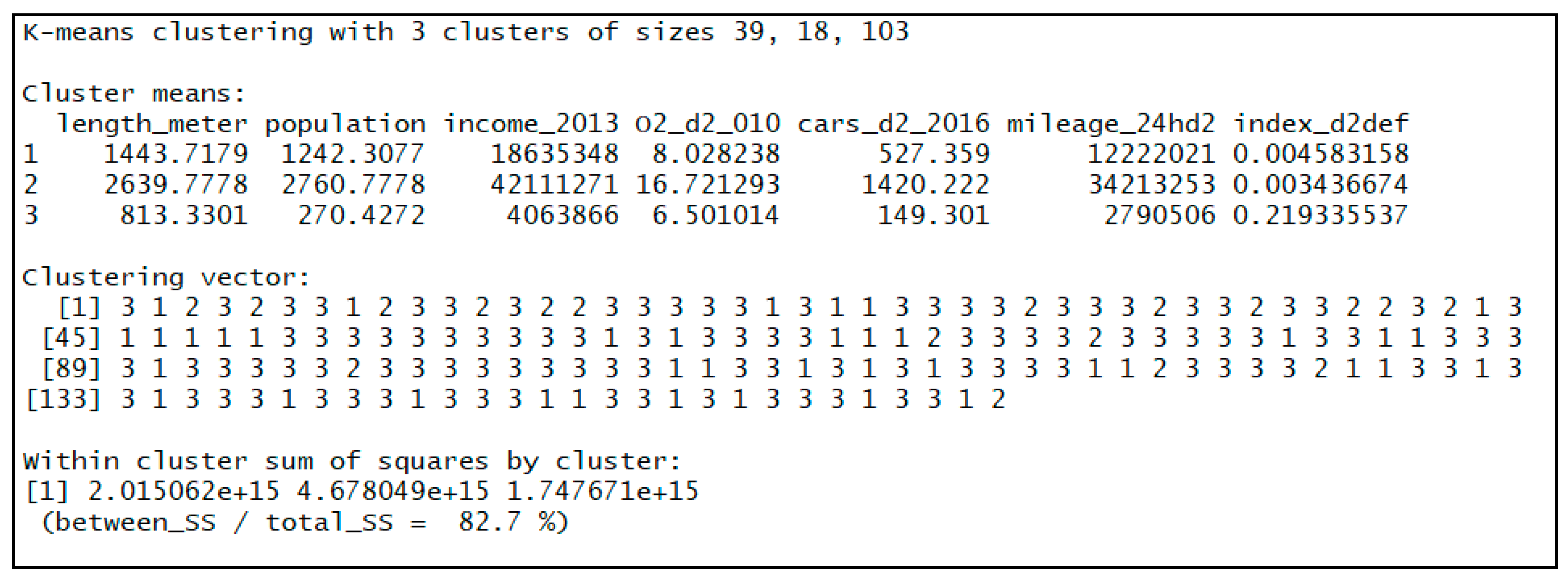
For the dt2 scenario, following data mining clustering through K-means, on a predefined number of 3 clusters, we obtained the following results (Figure 6):

Cluster #1 contains 39 instances (streets). We can see that the streets in this cluster have a sequestration index value (index_d1def) of 0.0045.

Cluster #2 contains 18 streets. The streets of this cluster have the smallest values of the sequestration index (index_d1def) of 0.0034. These areas are the most polluted ones.

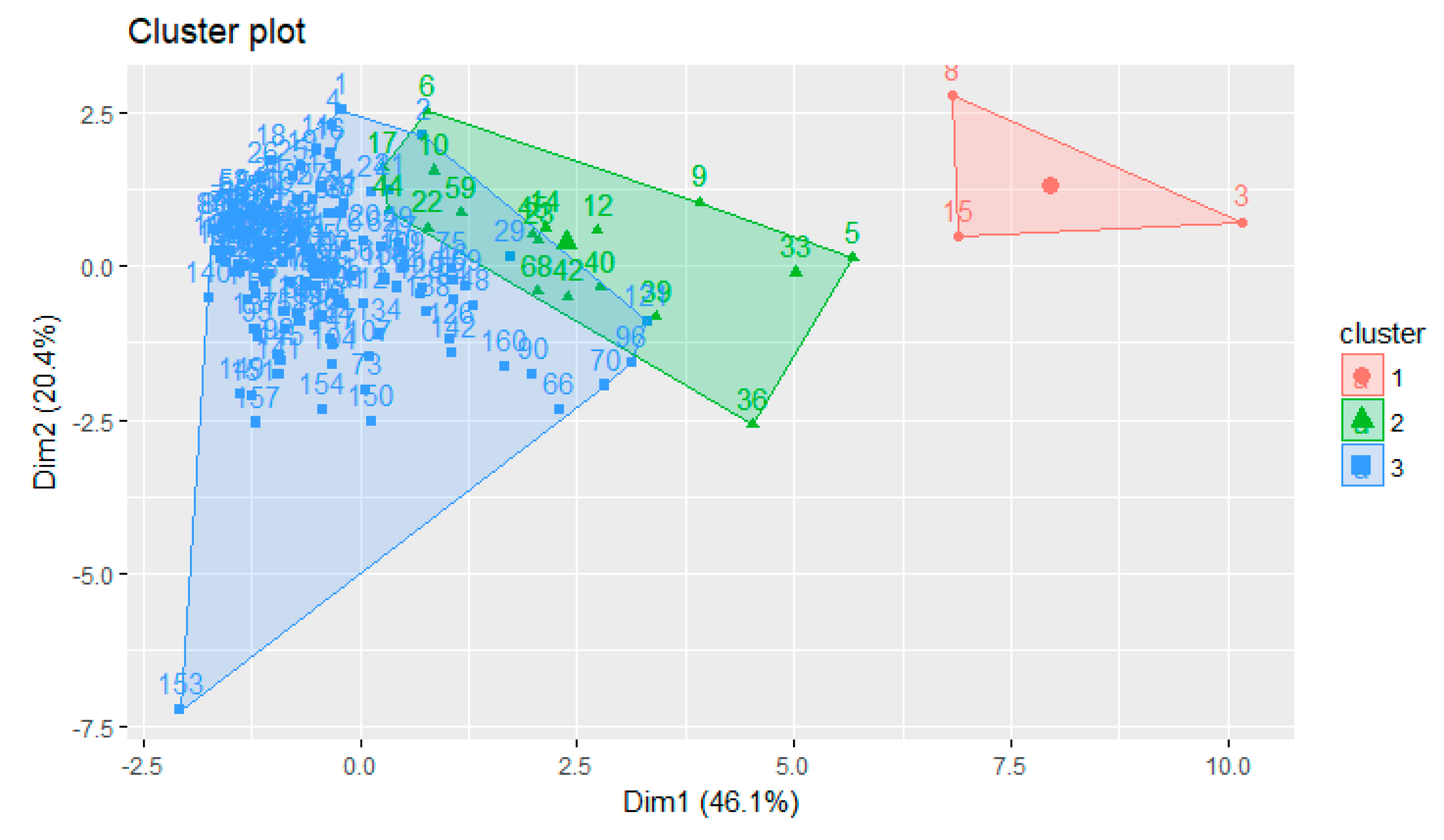
Cluster #3 has the highest number of streets (103). The centroid of this cluster has a CO₂ sequestration index value (index_d2def) of 0.219335537, significantly better than the other clusters by 0.21.

Figure 7 shows the “Cluster plot” graph. As in the dt1 scenario, cluster 3 has the highest number of streets.

We modeled the clusters for one day during the vegetation season (15 April–15 September). The flow-funds model provided the framework for traffic analysis and partial sequestration of carbon for 160 street areas, which cover over 50% of the mileage.

The carbon sequestration index in the dt2 scenario is 1.73 times greater than in the dt1 direction. The modeling of the sequestration index is made without five streets with people and car at a minimum level. The sequestration index of dt2 is higher, partly due to half mileage for this scenario. To synthesize, the low level of sequestration index in both cases is due to the low production of O₂ on the street areas. In both scenarios, we considered the same O₂ production for d1 and d2.

3.3. Clusters Spatialization

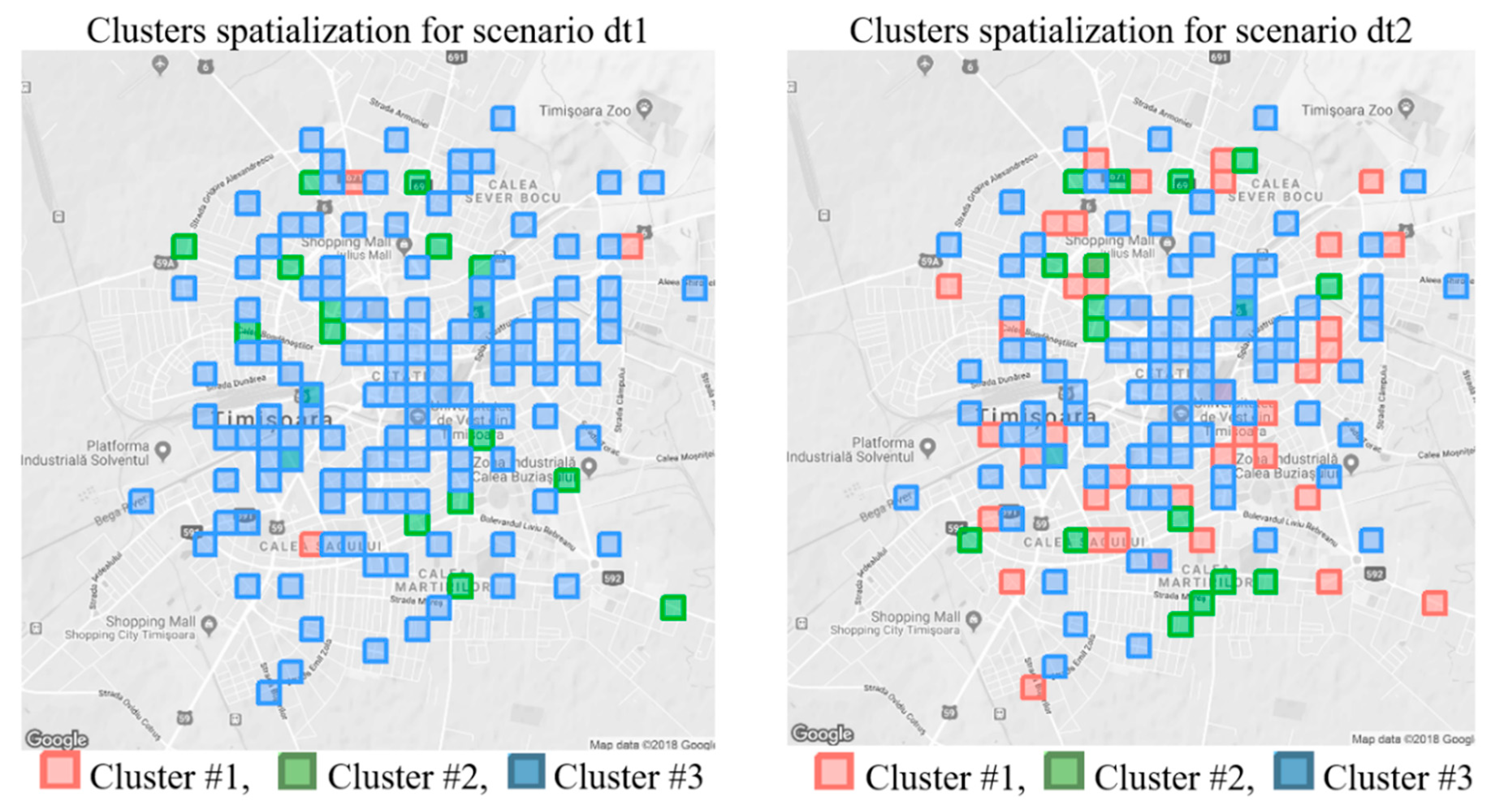
BDA has a central role in spatial data representation. We can see the spatial distribution of clusters on the streets for each of the two scenarios to ensure optimal decision support (Figure 8).

Cluster #1 (red color) of the dt1 scenario contains the streets of the main entry/exit points of the city. These traffic areas are the longest and busiest of the 160 streets.

Grouping the 160 main streets in clusters gives us a first analysis that can be used by decision-makers. In the first case (dt1), the three streets of cluster 1 concentrate 27.6% on mileage. The cumulative sequestration index is only about 0.04% for the three streets. The working document Vision 2030 traffic for Timisoara was developed using the DECLIMURB (DEcoupling and CLIMate change in URBan areas) database of West University of Timisoara, to achieve the carbon-neutral level. This target is to increase alternative transport by 2030: for public transport by 1.24 times, for cars-RES (electric, etc.) by 1.2 times, for bicycling by 1.84 times, and for walking by 1.55 times. The metrics modeled inside the DECLIMURB database were used for Report 4192 of the Nicholas Georgescu-Roegen Interdisciplinary Platform [38] for issuing by the Romanian Ministry of Environment (regional institutional unit) of Local Environment Permit no 1/2017 [10] for the new building code of Timisoara (acc. to Romanian rules, The General Urbanistic Plan) [12]. Another sub-option for carbon-neutral level is to reduce daily mileage through various restrictions, for example, by blocking traffic during rush hours in the core of the city [39]. The increase of urban tree inventory (LAI) for Timisoara is another basic requirement for decreasing the heat wave impact [37].

We performed the modeling of O₂-pollution processes on streets and related variables for a regular (average) day in the warm season. Passing the modeling of O₂-pollution flows to another month of the hot/cold season is possible. Switching to a monthly or yearly flow can be done by stoichiometric shaping of the metrics. For one month in the vegetation season, the calculation is similar. The 150-day vegetation season overlaps 75–90% with the warm season. For one month in the cold season, net O₂ production is considered zero. For one month or a few days in both seasons, the formulas apply accordingly. For one year, the pollution is modeled for 300 days with normal flow and the production of O₂ during the vegetation period.

3.4. Limitations

The cluster modeling used data for different years between 2011–2016: traffic flow (2011), population (2016), oxygen production (2013). To maintain all 160 streets in the dt2 analysis, we considered the minimum level of one car for the four car-free streets. The small number of cars generates high oscillation of the carbon sequestration index in the dt2 scenario. The same situation was for the population with a minimum level of people characteristics for nine streets. The sequestration index was consequently biased by considering the minimum level of these two variables.

4. Conclusions

The research has two findings: (1) modeling simultaneously for distinct whole streets using Roegenian processes with integration of effective O₂ production and pollution flows, the metrics of two sequestration indexes using neutral CO₂ point of reference instead of relative neutral CO₂; (2) simultaneous index modeling of O₂-pollution flows for actual street traffic and comparatively for garage-owner traffic with two cluster-based scenarios (dt1 and dt2). The two-fold perspectives of pollution integrated with O₂ tree production achieve an integrated framework for the next decisions for decreasing pollution.

The two indexes range between 4.29 × 10⁻⁶ (scientific form) and 0.437 for the dt1 scenario and between 9.18 × 10⁻⁶ and 11.78 for the dt2 scenario. The comparative analysis proposed in the research stimulates discussions between the anthropomorphic agents, individual or collective: people, firms, City Hall, local council, the public transport company, bicycling NGOs, and environment protecting NGOs. The total CO₂ sequestration for the whole street based on the two scenarios becomes the essential reference point for public decisions. Considering these results, some effects for the city are expected to reach some local targets to decrease pollution [10]. In other research, the metrics for urban streets include social, environmental, and health characteristics using deep learning and street imagery [23]. A direct measure could be the taxation of residential people according to each car’s actual mileage. In this case, local gas stations in the city ought to record the vehicle number on the fuel bill. Quarterly or at least two times per year, a progressive differentiated tax, established in relation with the mileage achieved, will be charged. The Ministry of the Environment could establish this rule and, distinctively, similar rules for pollution found in residential building areas [40].

The two-fold perspectives of the RCPS (dt1) and SPS (dt2) analysis based on Roegenian integrated flows of O₂ pollution offer support at a micro-scale level for decision-makers to identify solutions for street traffic and green inventory infrastructure for Timisoara within the main urban traffic area. The model offers a powerful tool for local decision making and for urban environmental policies using street traffic optimization to reduce CO₂ pollution.