Roles of Psychological Resistance to Change Factors and Heterogeneity in Car Stickiness and Transit Loyalty in Mode Shift Behavior: A Hybrid Choice Approach

Abstract

To support the scientific policy making and planning for promoting the share rate of sustainable public transit in urban areas of large metropolises, this study analyzes the influences of psychological resistance to change factors on commuters’ mode shift behavior while some external changes happen in the transport supplies. The heterogeneities in the car users’ stickiness to car and the metro users’ loyalty to metro are examined to support individual-specific travel behavior prediction. Web-scripted efficient experimental stated preference surveys including four commuting modes and three key factors are generated, and face-to-face interviews are conducted to collect reliable behavioral data. A hybrid choice approach, simultaneously considering the latent variables and quantitative level-of-service variables of different options, is employed for analysis. The results indicate that psychological resistance to change factors (routine seeking, cognitive rigidity, and emotion reaction) have significant and substantial influences on car users’ inclination to previously used commuting mode (i.e., car) in mode shift behavior. Car users with stronger routine seeking, stronger cognitive rigidity, and less emotion reaction show more predilection to car. Car users’ income level, gender, marital status, commuting distance, commuting time, license type, and flexible work time are found to partially explain the heterogeneity in car stickiness. In-vehicle crowding of public transit is a much more crucial factor for attracting car users to shift to public transit as compared to cost and travel time. Metro users with stronger routine seeking and less emotion reaction present a stronger inclination to metro in mode shift behavior. The influences of psychological resistance to change factors on metro users’ mode shift behavior are comparatively smaller than the influences of these factors on car users’ behavior. Metro users’ age, education level, commuting distance, commuting time, occupation, and flexible work time are identified to be associated with predilections for metro.

1. Introduction

Excessive car usage is related to higher negative consequences in terms of traffic congestion, air pollution, and accidents as compared to more sustainable public massive transit. Reducing private car usage and promoting the share rate of public transit is generally regarded as an important contribution for relieving the transport issues in urban areas. It is imperative to make managements for adjusting the mode split structure to improve the quality and sustainability of the urban transport system in metropolises with a huge population. The transport administrative in Shanghai has implemented several transport policies aiming at shifting car users to public transit including establishing public transit facilities (e.g., bus rapid transit, metro system, and Park and Ride) and license plate auction to control the number of private cars in the last decade. Nevertheless, car ownership was continuously increasing from 3.28 million in 2014 to 4.69 million in 2017 [1], which led to severer traffic problems and substantial societal welfare loss. Transportation managers in Shanghai are eager to understand the underlying reasons for previous policy failure and are thirsty for efficient measures of cutting down car usage. These need in-depth insights yielding principles of travelers’ mode shift behavior.

Some attractive characteristics of private car in level-of-service variables like flexibility, comparatively shorter travel time due to driving directly to the destination, and comfortable environment may result in travelers’ predilection to using car. These quantitative advantages of using a car can be nicely modelled by conventional microeconomic techniques like expected utility theory. Numerous studies have been conducted to quantify to what extent the travelers value different level-of-service attributes in mode choice behavior. Besides the objective or “hard” factors leading to travelers’ preference for car, plenty of works have investigated the “soft” or subjective factors of car stickiness like attitude, perceptions, and norms using social-psychological approaches including norm-activation model and theory of planned behavior. Steg [2] examined the various motivations for car uses in Groningen and Rotterdam, Netherlands. He concluded that besides the instrumental aspects of car use like travel time and comfortable features, the symbolic and affective attitudes attached to cars (e.g., car is a representative of social status and power) significantly contributed to the positive utility of driving a car. De Groot and Steg [3], as well as Rieser-Schüssler and Axhausen [4], reported that travelers with pro-environmental cognitions tend to use cars less frequently. Bamberg et al. [5] used datasets collected in two German urban agglomerations to investigate the impacts of personal norms (e.g., sacrificing personal interests for benefit of others) on intention to use public transit and found that personal norms played a significant role in predicting travelers’ public transit uses after controlling the effects of attitude and perceived behavioral controls. García et al. [6] studied the effects of cognitive, affective, and behavioral attitudes towards the use of walking and cycling on both intentions and real use of different transport modes. The results indicated that cycling and walking were evaluated differently in terms of feelings of freedom, pleasure, and relaxation. Positive evaluation of past walking behavior was negatively associated with both the intention to walk and actual walking. Cheng et al. [7] examined the effects of latent attitudinal variables and sociodemographic differences on travel behavior. They revealed that ensuring high comfort, convenience, moderate safety, and reliability were attractive methods of promoting usage of public transport. Some other subjective factors were also found to influence the degrees of car stickiness. Bergstad et al. [8] examined the socio-demographic variables on daily car use in Sweden and demonstrated that households with children or living in the rural areas had comparatively stronger car stickiness. Nordfjærn et al. [9] found that travelers with higher income showed more preference for car usage.

In the psychological and behavioral literature, one factor that is generally recognized to block a change in behavior is the psychological resistance to change [10,11]. The resistance to change denotes the traveler’s pre-disposition to resist changes or the inevitability of behaving in a certain way [10,12]. If a traveler holds negative opinions about changes in their daily routine and experiences distressed emotions due to the occurrence of changes, the individual may be more reluctant to think about a change in behavior. The impacts of resistance to change on behavior have been investigated in management science [13], sociology [14], and psychology [10]. To our best knowledge, no empirical studies have quantitatively examined the role of psychological resistance to change and to what extent it influences travelers’ willing to change in mode shift behavior when some changes happen in transport supplies. Nordfjærn et al. [11] tested the relationships of habit and resistance to change with car users’ intention to use public transit using theory of planned behavior framework without considering the level-of-service variables in modeling. However, they focused more on the causal relationships among different subjective factors. 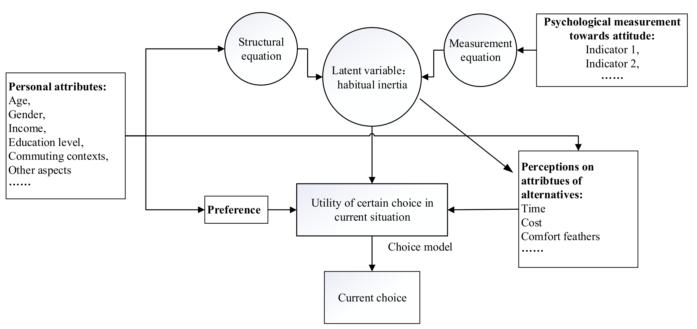In this study, we investigate the impacts of psychological resistance to change factors on mode shift behavior by applying the hybrid modeling approach [15] that integrates the discrete choice model and latent variable model. The framework of hybrid choice model (HCM) is illustrated in Figure 1. The hybrid choice approach can incorporate the latent variables and observed level-of-service variables of different options to quantify the influences of various factors on travel behavior. The HCM is also recognized to be helpful to structure the respondents’ heterogeneity more efficiently and intuitively as compared to mixed logit model with interactions of personal attributes [16]. Taking advantage of HCM, we explore the direct effects and indirect effects of personal characteristics on car stickiness to investigate the heterogeneity among car users for individual travel predictions.

Besides HCM, the system dynamics model is another alternative for describing travelers’ behavior changes responding to transport supply adjustments and the dynamic transportation system [17]. The system dynamics model (SDM) uses stocks, flows, internal feedback loops, and the set of various variables and equations based on quantitative and qualitative information to model and simulate the nonlinear behavior of complex systems over time. For instance, Lei et al. [18] used SDM to simulate an urban low-carbon transport system and indicated that the rapid increase of private car was a crucial contributor to carbon emission. Acharya [19] employed the SDM to explore the influences of some commonly discussed policy alternatives and demonstrated that an off-road rapid transit system was beneficial for maintaining the share rate of public transport and relieving traffic congestion. We will compare the SDM and the HCM in terms of analysis level, focus and advantages, modeling methodology, and calculation. 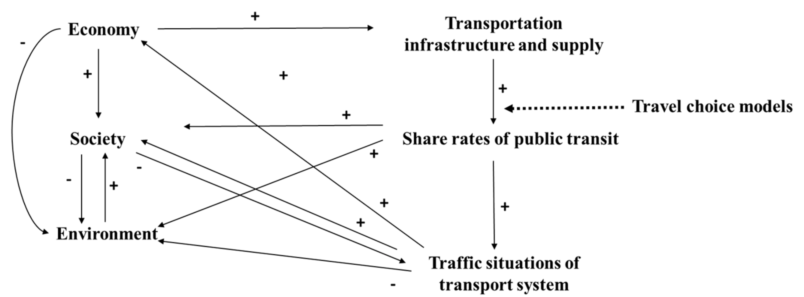Figure 2 illustrates an example of a system structure including the economy, society, transportation system and environment, and their causal relationships where the arrow denotes the causal effect and the sign demonstrates whether the effect is positive or negative. In the analysis level, SDM has the advantages of dealing with interactions, nonlinear problems, information feedback, and dynamic complex among subsystems, and thus is generally used as a tool to investigate the macroscopic effects of policy and management in the transportation literature. The HCM mainly addresses the principles of every single individual’s travel choice behavior at a comparatively more microscopic level and is used to obtain the overall traffic demand by accumulating the predicted behavior of each traveler [20]. For instance, the SDM can analyze how the changes in the transportation system in Figure 2 will affect other components (e.g., society, economy, and environment) in the total system in a macroscope level, while the HCM investigates the individuals’ response to the changes in transport supply and then gets the share rate of each transport mode. This leads to the differences in the analyzing focus and advantages of SDM and HCM. The SDM is superior in simulating complicated interactions, feedback loop, and dynamics in a system with different aspects (e.g., economy, society, transportation, and environment) and analyzing the derivative influences of changes in the subsystems by a continuous view over time. However, HCM concentrates more on revealing the principles about how travelers make their travel choices and quantifying the influences of different factors on travelers’ behaviors (e.g., the weights of level-of-service variables and to what extent travelers’ attitudes influence their choice), which can be used to predict the spatial-temporal demand in the transportation network. The HCM is generally applied for describing the travelers’ behavior in a time section, and can be extended to describe dynamic behavior over time by adding dynamic processes [21]. For the modeling methodology, the SDM uses the so-called causal loop diagram and stock-flow diagram to qualitatively and quantitatively construct the structure of a system. More specifically, the causal loop diagram explicitly describes the nonlinear causality among the relevant stakeholders in the system, as shown in Figure 2, and establishes the evident feedback loops, while the stock-flow diagram defines the states and variables of stocks, the quantitative control rules, and feedback mechanisms based on differential or integral equations [22]. 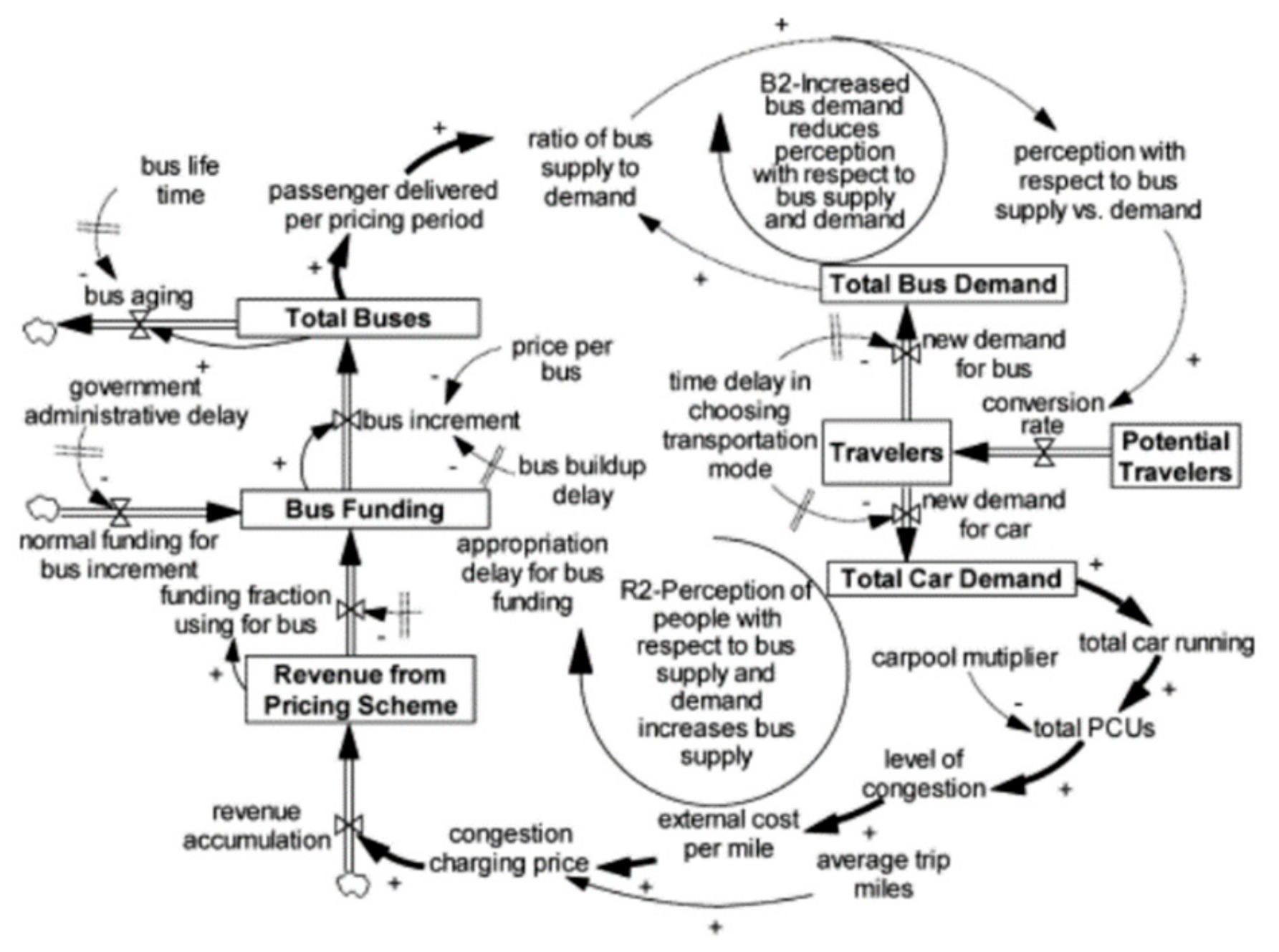Figure 3 shows an example of a stock-flow diagram for investigating the mode choice behavior under the congestion pricing provided by Liu et al. [23]. In the stock-flow diagram, the relationship between demand for bus and the perceived service level of bus (measured by linguistic or categorical variables) is described and reflects the dynamic interactions over time but is not used to predict the statistical demand for the bus. Nonetheless, the HCM using the framework in Figure 1 and behavioral theory (e.g., utility maximization or regret minimization theory) model the individuals’ choice behavior and generally aims to predict the statistical demand for transport models at a more microscope level. Even though the SDM and HCM can be somehow combined by agent-based modeling and simulation with much complexity (see a study by Flynn et al. [20]), the fundamental theory and original purposes of the SDM and HCM are distinct. For the model estimation and calculation, the SDM commonly turns to the specific computer software (e.g., VENSIM) due to the dynamic and simulation characteristics, while the HCM falls back on the analytical and numerical calculation. This study mainly concentrates on quantitatively analyzing the influences of psychological factors and heterogeneity in the travel behavior and thus adopts HCM for analysis. The results from HCM can be useful inputs for simulating a dynamic transportation system to explore the dynamic travel behavior changes.

Compared to numerous studies focusing on enticing car users away from private cars, little work has been devoted to investigating travelers’ loyalty towards public transport. In recent decades, the issue that plenty of public transit users shift to private transport becomes more and more noticeable since economic growth and emerging car-sharing services in China enable the private transport service to be affordable and accessible to previous public transit users. The transit loyalty is defined as the intention to future usage and willingness to recommend public transit to others [24]. Van Lierop et al. [24] conducted a comprehensive review regarding the influences of service factors on transit loyalty and compared the importance of different influencing factors. Service factors including on-board experience, service delivery, waiting conditions, transfers, customer service, and cost have been found to influence transit users’ loyalty [24]. Weinstein [25] indicated that in-vehicle cleanliness and comfort significantly influenced travelers’ perceived on-board experience. De Oña [26] found that the waiting conditions and on-board information were important factors influencing the transit users’ travel experience. Nevertheless, it was noted that travelers’ perceived utility towards transport modes were determined by both objective factors and subjective factors [27]. Most literature explored the effects of objective factors (e.g., service quality factors) on transit loyalty, while the subjective factors were comparatively seldom investigated. In this study, we examine whether the psychological resistance to change factors play roles in transit loyalty and preventing transit users from shifting to private transport. We investigate the effects of various factors (e.g., demographic attributes, commuting contexts, and time scheduling factors) on heterogeneity of transit users’ loyalty towards public transport. The results will shed light on understanding the underlying effects of psychological resistance to change factors on mode shift behavior and explaining the travelers’ heterogeneity in mode shift behavior. The results can support transport practitioners to make operational instruments for adjusting mode split structure based on individual preference characteristics.

The remainder of this paper firstly gives the survey design and data collection process, followed by descriptions towards the modeling framework of HCM in Section 3. The analysis results and discussions are presented in Section 4, followed by concluding remarks.

2. Survey Design and Data Collection

The used databank herein is a survey regarding commuting mode shift behavior collected in 2017, Shanghai of China. The survey contained two stages.

In the first stage, information about the respondent’s current commuting trip was collected including the frequently used transport mode, the range of travel time, overall cost, commuting distance, and comfort features. The revealed information concerning other available modes for commuting was gathered as well.

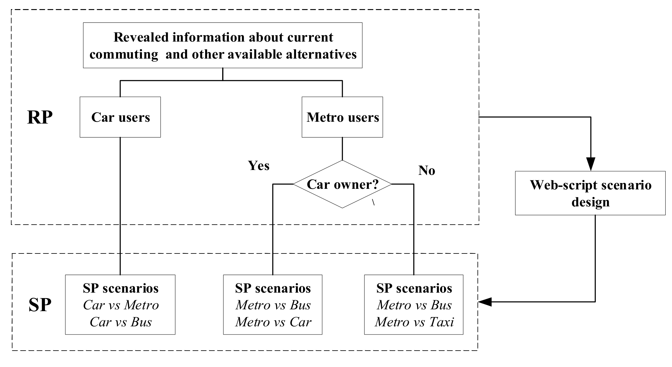
In the second stage, the stated preference (SP) questionnaire was generated immediately using web-scripted code by mobile devices based on the individual revealed information and presented to the same respondent. The questionnaire contained three parts: (1) A brief introduction to the survey; (2) SP choice scenarios; (3) personal information. 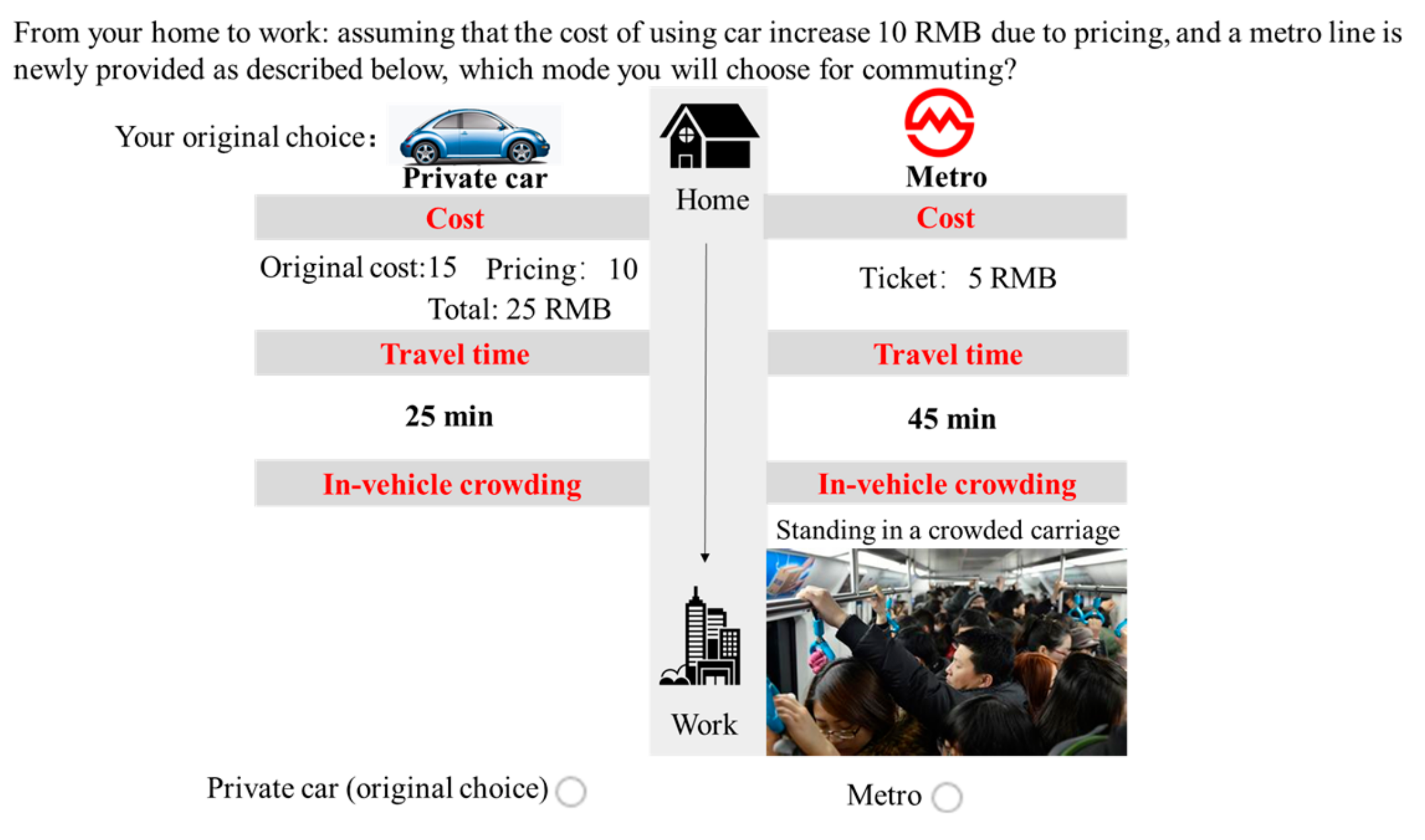The procedure for generating SP scenarios is demonstrated in Figure 4. The SP scenario is a choice between the current commuting transport mode and a new hypothetical alternative. The cost of the previously used mode was assumed to increase due to pricing strategy. One example of the scenarios is shown in Figure 5. Four commuting modes (private car, metro, bus, and taxi) were considered. The considered attributes influencing mode choice in the SP scenarios were cost, in-vehicle crowding, and travel time. For car users, the available alternatives were car, metro, and bus. We asked the mode shift scenarios of car and metro at first and then asked the scenarios of car and bus. For metro users, if the respondent had access to a private car, the available three alternatives were car, metro, and bus. Otherwise, the available options were the taxi, metro, and bus. The setting of attribute levels for scenario design is shown in

Table 1. Attributes and their levels in SP scenario design.

	Alternative	Attributes	Levels
Car/Taxi users	Car/Taxi (original mode)	Travel time	RP_time
		Cost (petrol, parking fare, tolls)	RP_cost + [5, 15, 25, 40]
		Crowding inside car	None
	Metro	Travel time	RP_time× [0.8, 1.1, 1.4]
		Cost (ticket)	[3, 4, 5, 6]
		Crowding inside metro	[Level 1, Level 2, Level 3]
	Bus	Travel time	RP_time ×[1, 1.3, 1.6]
		Cost (ticket)	[2, 4, 6]
		Crowding inside bus	[Level 1, Level 2, Level 3]
Metro users	Metro (original mode)	Travel time	RP_time
		Cost (ticket)	RP_cost + [2, 6, 10]
		Crowding inside metro	RP_crowding level
	Bus	Travel time	RP_time [0.75, 1, 1.25]
		Cost (ticket)	[2, 4, 6]
		Crowding inside bus	[Level 1, Level 2, Level 3]
	Car	Travel time	RP_time × [0.7, 0.9, 1.1]
		Cost (petrol, parking fare, tolls)	Cost_petrol + [5, 10, 20]
		Crowding inside car	None
	Taxi	Travel time	RP_time ×[0.7, 0.9, 1.1]
		Cost (ticket)	[T1, T2, T3]
		Crowding inside taxi	None

Note: RP_time, RP_cost, and RP_crowding denote the gathered actual travel time, cost, and in-vehicle crowding for the respondent’s commuting. Crowding Level 1: Uncrowded with seats; Level 2: Standing in not crowded carriage; Level 3: Standing in the very crowded carriage. Cost of metro is constrained by its travel time (TT) in design, when TT =< 25, the cost = 3; when 25 < TT < 35, cost = 4; when 35 < TT < 45, cost = 5; when TT > 45, cost = 6.The levels for the cost of taxi are calculated according to the pricing rules of DiDi company in Shanghai: T1 (hitchhiking) = distance × 1.6, T2 (car sharing with others) = 0.8 × (distance × 2.3 + travel time × 0.5), T3 (taxi without sharing) = distance × 2.3 + travel time × 0.5. The units for cost and travel time are CNY (1 CNY = 0.146 dollar) and minute.

. The attribute levels were determined based on the collected respondent’s reveal information in the first stage and the empirical knowledge from local transport practitioners. For instance, for car users’ scenario design, the levels of travel time by car were set based on the revealed commuting time; the levels of increased cost of using a car included four levels fluctuating from 5 to 40 RMB; the levels of travel time for metro were set based on revealed information; the levels of cost by metro and bus were the real ticket price in Shanghai; three levels reflecting three typical in-vehicle crowding situations during commuting in Shanghai were set for the in-vehicle crowding in metro and bus. The statistical content design of SP scenarios refers to D-error efficient design method [28] ensuring orthogonality and utility balance among alternatives. The details about D-error efficient design method are available in the study of Rose et al. [28]. For each type of mode shift situation, 12 scenarios were generated as the database and four scenarios were randomly selected to give out to each respondent in case of excessive workload. Graphic images instead of word descriptions for different crowding levels were presented in the SP scenarios to promote understandability [27].

The respondents’ personal characteristics including demographic attributes (e.g., gender, age, occupation, education level, income, place of residence, marital status) and other information (e.g., psychological resistance to change factors and schedule flexibility for work) were also collected.

To measure the latent psychological resistance to change factors, we applied a set of previously validated instruments proposed by Oreg [29]. The psychometric items have been used to measure how resistant people are to change in different choice contexts. Oreg [29] tested the measurement items for change-resistant behavior across a variety of contexts and reported that the measurements performed quite well in quantifying the psychological resistance to change across different types of behavior. These measurement items were also validated by Nordfjærn et al. [11] in the context of travel behavior. Questions such as “I prefer having a stable routine to experiencing changes in my life” and “Often, I feel a bit uncomfortable even about changes that may potentially improve my life” were presented to the respondents. The respondent was asked to report their levels of agreement on such statements by a five-level Likert Scale (i.e., strongly disagree (1), slightly disagree (2), neutral (3), slightly agree (4), strongly agree (5)).

A localized pilot survey was executed in advance to test the validity of survey design and to renew the prior parameters in the design. Both online and face-to-face interviews were conducted to collect data. Nevertheless, the collected data from online surveys were not as reliable as those from face-to-face interviews. Therefore, investigators were recruited to conduct face-to-face and one-to-one surveys for the sake of validity and representativeness of data. The surveys were carried out in public locations (the Hongqiao Transportation Hub and the Bureau of vehicle management) to achieve a wide geographical coverage of various respondents as much as possible in case of biases. The Hongqiao Transportation Hub is the largest comprehensive transportation junction in Shanghai connecting Hongqiao airport, Hongqiao railway station, and Hongqiao public transit center. The Bureau of Vehicle Management is the department responsible for car license application, driver license application, and administration of the traffic violation. Investigators were trained about how to conduct the survey properly using mobile devices. Respondents were asked to read and understand questions carefully, and to answer according to their own actual preferences. People over 60 years old were rejected for participation due to a high probability of retirement. Some souvenirs were given to the respondents for gratitude of participation. Finally, 525 valid respondents and 4200 SP observations were collected. The sample sizes for private car users and metro users are 300 and 225, respectively. The respondents’ statistical attributes are summarized in

Table 2. Statistical summarization of the sample and classifications.

Personal Attributes	Statistics	Classifications and Coding of Variables
Age	Less than 30 years old (47.8%), 30~40 (40.5%), 40~50 (9.6%), more than 50 years old (2.1%))	Age (<30): Control group; age (30~50): Equals 1 when age is between 30 and 50, otherwise is 0; age (>50): Equals 1 when age is more than 50, otherwise 0. The coding of dummy variables below is similar.
Education level	Lower than undergraduate (25.4%), Undergraduate (57.1%), Master (14.9%), Doctor (2.6%)	Less than undergraduate: Control group; undergraduate; master; doctor.
Monthly income (RMB)	Less than 3000 (2.2%), 3000~6000 (15.1%), 6000~10,000 (32.4%), 10,000~20,000 (29.3%), more than 20,000 (21%).	Monthly income (<6000): control group; Monthly income (6000~10,000): 0.8; Monthly income (10,000~20,000): 1.5; Monthly income (>20,000):2.5.
Gender	Male (65.5%), female (34.5%)	Female: control group; male.
Occupation	State-owned enterprise (29.7%), Private enterprise (43.3%), Individual operation (8.4%), others (18.6%)	State-owned enterprise; private enterprise or others: Control group.
Marital status	Yes (66.2%), No (33.8%)
Commuting distance	Less than 5 km (14%), 10 km (29.1%), 10~20 km (35.8%), over 20 km (22.1%)	Commuting distance (<10 km): control group; commuting distance (10~20 km); commuting distance (>20 km).
Commuting time	Less than 30 min (46.6%), 30~60 min (37.6%), more than (15.7%)	Commuting time (<30 min): Control group; commuting time (30~60 min); commuting time (>30 min).
License type	No car (30.1%), Type1 (46.7%), Type2 (7.8%), Type3 (15.4%)	License Type1; others: control group.
Flexible work time	Yes (30.6%), No (69.4%)	No: control group; yes.

Note: The value of parameter for the monthly income is the mean income of each classified group with a unit of 10,000 CNY. The license type1 is limited in Shanghai, is worth over 10,000 dollars, and can only be obtained by monthly license auction. Only cars with license type1 are allowed to use the express roads in peak hours and other private cars cannot use express roads in peak hours.

. The collected data cover various travelers in terms of age, income, education level, and commuting distance and there are not obvious biases in the respondents’ characteristics.

Table 2 also presents the classifications of all the personal attribute variables that will be used in later modeling specifications. The person attribute variables are all coded with dummy variables for considering potential nonlinear effects of personal characteristics [30]. For instance, for the coding of age, the variable “age (30~50)” is 1 when the respondent’s age is between 30 and 50, otherwise it is zero; the variable “age (>60)” is 1 when the respondent’s age is over 60, otherwise it is zero. The respondents with an age less than 30 are set to be the control group. A similar coding principle goes for all other considered factors in the models except monthly income. The criterions for the classifications are according to the way commonly used in various research [31,32] and the generally recognized classifications in China. The value of parameter for the monthly income is the mean income of each classified group with a unit of 10,000 CNY [33].

3. Modeling Framework and Specifications

3.1. Factor Analysis of Latent Variables

To validate the efficiency of measurement items regarding psychological resistance to change factors, we conducted a reliability test for the internal consistency of the responses among the measurement items. The Cronbach’s alpha for the received responses is 0.83, which is higher than the recommended threshold (0.7). This indicates that the internal consistency of the used measurement items about psychological resistance to change factors is satisfying and the results can be confidently used for further analysis.

Afterwards, an exploratory analysis was executed to extract the main attitudinal factors from the measurement items. Several rotation procedures were tested and the varimax rotation gave best performances in terms of explaining variance in the data. Finally, three main factors with eigenvalues over 1 were identified. The results of factor analysis are shown in

Table 3. Results of factor analysis.

Items		Factor1	Factor2	Factor3
S1	I generally consider changes to be a negative thing	0.710	-	-
S2	I prefer having a stable routine to experiencing changes in my life	0.804	-	-
S3	If my life forms a stable routine, I look for ways to change it	−0.596	-	-
S4	I’d rather be bored than surprised	0.775	-	-
S5	If I were to be informed that there’s going to be a significant change regarding the way things are done around me, I would probably feel stressed	-	0.812	-
S6	When I am informed of a change of plans, I tense up a bit	-	0.908	-
S7	When things don’t go according to plans, it stresses me out	-	0.889	-
S8	Once I’ve made plans, I’m not likely to change them	-	-	0.449
S9	Often, I feel a bit uncomfortable even about changes that may potentially improve my life	0.706	-	-
S10	I sometimes find myself avoiding changes that I know will be good for me	0.628	-	-
S11	My mind is easily influenced by others		-	−0.549
S12	Once I’ve come to a conclusion, I’m not likely to change my mind	-	-	0.802
S13	My views are very consistent over time	-	-	0.642

Note: Kaiser–Meyer–Olkin test: 0.84, Bartley sphere test: ${\chi }^2$ (12982.681), df (78), sig (0.000).

. The three main factors can explain 62% of the variance of the data, which is quite good. The first factor is explained by measurement items S1, S2, S3, S4, S9 and S10. According to the questions, the first factor mainly describes the individual’s unwillingness to change his/her current statue and thus is named as “Routine Seeking”. The second factor explained by S5, S6, and S7 reflects the individual’s emotional reaction when unexpected changes happen and is called as “Emotion Reaction”. The third factor represents the degree of easily changing way of thinking and thus is named “Cognitive Rigidity”. The three factors are all related to the psychological resistance to change and may have potential influences on travelers’ mode shift behavior.

3.2. Hybrid Choice Model Specification and Estimation

For the modeling, we employed the hybrid choice modeling approach with the random utility-maximization (RUM) framework that considers users’ heterogeneity, latent variables, and panel effects [34]. The integration of latent variable into RUM model is one of the typical applications to account for the effects of individual’ latent factors that are difficult to be directly observed on the choice process. As shown in Figure 1, the HCM framework integrates two parts: The latent variable model (LVM) and the discrete choice model. In the LVM, the structural models relate the measurable personal characteristics to the values of latent variables, whereby the measurement model links the latent variable with indicators in the measurement items. The attitudinal part of LVM is generally represented by a multiple-indicator multiple-cause model [35].

The utility of transport mode n for individual i whose previously used mode is mode k can be given by Equation (1):

$$\begin{array}{l}{U}_{ki}=\underset{V_{ki}}{\underbrace{{\beta }_{cost}*cos{t}_{ki}+{\beta }_{time,k}*tim{e}_{ki}+{\beta }_{crowd,k}crow{d}_{ki}+u_{lv}L{V}_i+{\displaystyle \sum _z{\xi }_z{Z}_{zi}}+AS{C}_k+{\sigma }^2{}_k}}+{\epsilon }_{ki}\\ U_{ni}=\underset{V_{ni}}{\underbrace{{\beta }_{cost}*cos{t}_{ni}+{\beta }_{time,n}*tim{e}_{ni}+{\beta }_{crowd,n}crow{d}_{ni}+AS{C}_n}}+{\epsilon }_{ni}\hspace{1em}(n\ne k)\end{array}$$

(1)

where the $cos{t}_{ni}$, $tim{e}_{ni}$, and $crow{d}_{ni}$ are the cost, travel time, and in-vehicle crowding. Two dummy variables are used to account for non-linear effects in the in-vehicle comfort features. The parameter of crowding level 2 equals to one if the level of crowding is “standing in not crowded carriage” and zero otherwise. The same goes for in-vehicle crowding level 3. The crowding level 1 was the “good enough” situation and set as the reference. LV_i is the investigated latent variable including “Routing Seeking”, “Emotion Reaction”, and “Cognitive Rigidity”. $Z_{zi}$ is the vector of personal attributes. $AS{C}_k$ is the alternative-specific constant to measure the unobserved preference for an alternative. ${\sigma }^2{}_k$ denotes the unobserved variances for alternative k and is assumed to be normally distributed with a zero mean. ${\epsilon }_{ki}$ is the unobserved error component and is set to be identical and independent to the Gumbel distribution.

The structural equations for latent variables can be expressed by a linear function of observed personal characteristics for individual i as Equation (2) [30].

$$L{V}_i={\displaystyle \sum _z{\rho }_z}{Z}_{zi}+{\eta }_{lvi}{\eta }_{lvi}~N(0,{\sigma }^2{}_{lv})$$

(2)

where $Z_{zi}$ is the vector of personal attribute and ${\rho }_z$ is the corresponding coefficient vector. ${\eta }_{lvi}$ is the variance term with normal distributions. The measurement equation for the latent variable with responses to the s^th attitudinal measurement item $Indicato{r}_{is}$ can be given by:

$$Indicato{r}_{is}=\overline{Indicato{r}_s}+{\kappa }_{s}L{V}_i+{\phi }_s{\phi }_s~N(0,{\sigma }^2{}_s)$$

(3)

where ${\overline{Indicator}}_s$ is the mean value of the measurement item s over all individuals in the sample. ${\kappa }_s$ is the latent variable measurement coefficient and ${\phi }_s$ is the standard deviation (normally distributed with a zero mean) for item s. The individual i′s choice probability of mode n is defined as:

$$\begin{array}{ll}{P}_{ni}& =\mathit{Prob}\left\{U_{ni}\ge U_{nj}\right\}\\ & =\mathit{Prob}\left\{V_{ni}+{\epsilon }_{ni}\ge V_{nj}+{\epsilon }_{nj}\right\}\\ & =\mathit{Prob}\left\{V_{ni}-V_{nj}\ge ({\epsilon }_{ni}-{\epsilon }_{nj})\right\}\forall n,j\in C_i\end{array}$$

(4)

where $C_i$ is the choice set of individual i. Since ${\epsilon }_{ki}$ is set to be identical and independent to the Gumbel distribution, the $P_{ni}$ can be further calculated by the Logit formulation as in Equation (5)

$$P_{ni}=\frac{\exp (V_{ni})}{{\displaystyle {\sum }_{i=1}^N\exp (V_{ni})}}.$$

(5)

Given the actual choice consequences of individual i for Q scenarios $y_{iQ}$= [${\mathrm{y}}_{i1}$, …, ${\mathrm{y}}_{iq}$, …, ${\mathrm{y}}_{iQ}$], and the consequences of latent variable measurement items I_i, the likelihood function can be expressed by Equations (6)–(8).

$$\begin{array}{l}{L}_i\left( y_{iQ},I_i|{\beta }_{cost},cos{t}_{ni},{\beta }_{time,n},tim{e}_{ni},{\beta }_{crowd,n},crow{d}_{ni},u_{lv},{\kappa }_s,L{V}_i,{\xi }_z,{\rho }_z,Z_{zi},{\phi }_s ,{\eta }_v,{\sigma }^2{}_n\right) \\ ={\displaystyle \prod _{q=1}^Q\begin{array}{l}P({\mathit{y}}_{nQ}|{\beta }_{cost},cos{t}_{ni},{\beta }_{time,n},tim{e}_{ni},{\beta }_{crowd,n},crow{d}_{ni},u_{lv},L{V}_i,{\xi }_z,Z_{zi},{\sigma }^2{}_n)\\ *P(I_i|{\kappa }_s,L{V}_i,{\phi }_s )*P(L{V}_n|{\rho }_z,Z_{zi},{\eta }_v)\end{array}}\end{array}$$

(6)

$$P(L{V}_i|{\rho }_z,Z_{zi},{\eta }_v)~N({\rho }_z*Z_{zi},{\sigma }^2{}_v)$$

(7)

$$P(I_i|{\kappa }_s,L{V}_i,{\phi }_s)={\displaystyle \prod _{s=1}^S\mathsf{\Phi }(\frac{Indicato{r}_{is}-\overline{Indicato{r}_s}-{\kappa }_{s}LV}{{\sigma }^{}{}_s}}).$$

(8)

Due to the complexity of the model formulations, there is no closed form for the optimization. We employed the maximum simulated likelihood techniques [36] for estimation. The R software (version 3.5) was applied to conduct the model calibration process. Five hundred random draws were generated using the modified Latin hypercube sampling method [37] to simulate the random parameters in the model specifications. The panel effect among individuals was considered for keeping unobserved preference heterogeneity among individuals and preference homogeneity for one individual over a series of choices. The error component models were performed firstly to examine several possible nested structures among transport modes, and it turned out that there was a correlation between the metro and bus.

4. Results and Discussion

4.1. Car Users’ Mode Shift Behavior

The mode shift behavior of car users and metro users are analyzed separately since the influences of psychological resistance to change factors on mode shift behavior mainly represent the stickiness to or disposition to change previously adopted commuting transport modes. The results regarding car users’ mode shift behavior are summarized in

Table 4. Results of HCM for car users.

	Routing Seeking		Cognitive Rigidity		Emotion Reaction
Parameters	Coef.	z-Value	Coef.	z-Value	Coef.	z-Value
Cost	−0.082	−12.69	−0.0823	−12.56	−0.0811	−12.41
Travel time (car)	−0.0462	−2.37	−0.053	−2.59	−0.0494	−2.98
Travel time (metro)	−0.0429	−5.78	−0.0429	−5.78	−0.0425	−5.75
Travel time (bus)	−0.0561	−7.29	−0.0562	−7.29	−0.0559	−7.29
In−vehicle crowding level 2 (metro)	−1.3553	−5.64	−1.3662	−5.66	−1.3353	−5.56
In−vehicle crowding level 3 (metro)	−2.0023	−8.57	−2.0132	−8.62	−2.0034	−8.59
In−vehicle crowding level 2 (bus)	−1.0273	−4.35	−1.0193	−4.29	−0.9833	−4.15
In−vehicle crowding level 3 (bus)	−1.3043	−5.49	−1.2766	−5.39	−1.2615	−5.33
Correlation terms between metro and bus	0.5695	2.72	2.3727	13.99	0.8451	3.03
LV1: Routing seeking	0.3484	2.98
LV2: Cognitive rigidity			0.4153	3.01
LV3: Emotion reaction					−0.6512	−3.23
ASC (car)	2.477	3.77	2.7443	3.98	2.3118	3.39
${\sigma }_{car}$	2.2288	12.54	0.2971	1.10	2.1454	9.96
ASC (metro)	1.4254	4.53	1.4403	4.57	1.4328	4.56
ASC (bus)	0	fixed	0	fixed	0	fixed
Effect of personal attributes on utility of car
Monthly income	0.2856	1.95	0.2456	1.65	0.0052	0.03
Male	0.5213	1.67	0.3263	1.03	0.4233	1.39
Age (30~50)	−0.3587	−0.97	−0.5012	−1.3	−0.6065	−1.45
Age (50~60)	−0.0662	−0.06	0.0947	0.10	0.197	0.23
Education level (undergraduate)	0.4241	1.19	0.3184	0.91	0.4644	1.21
Education level (master)	0.0353	0.06	−0.2199	−0.40	−0.0008	0
Education level (doctor)	0.1399	0.14	0.068	0.08	0.276	0.31
Married	0.7489	1.85	1.1825	2.69	1.3476	2.99
Commuting time (30~60 min)	0.8189	1.54	1.0428	2.08	0.7155	1.43
Commuting time (>60 min)	1.3005	1.17	1.3683	1.29	0.8783	0.77
Commuting Distance (10~20km)	0.0491	0.11	0.1258	0.3	−0.0371	−0.09
Commuting Distance (>20km)	0.9767	1.64	1.4498	2.32	0.8632	1.48
License type1	0.8122	2.62	0.8627	2.67	0.6491	1.87
Working in SOE	0.028	0.07	0.0924	0.25	0.2122	0.63
Flexible work time	1.4701	4.82	1.005	3.34	1.1517	3.50
Observations	2400		2400		2400
Final log-likelihood of HCM	−3253.481		−2673.906		−2104.498
Final log-likelihood of choice model	−1163.685		−1165.053		−1165.646
Number of estimated parameters	53		49		47

Note: SOE denotes state-owned enterprise.

(results of HCM) and

Table 5. Results of latent variable models for car users.

	Routing Seeking		Cognitive Rigidity		Emotion Reaction
Parameters	Coef.	z-Value	Coef.	Coef.	z-Value	Coef.
Measurement Equations
${\kappa }_1$	1 (fixed)	-
${\kappa }_2$	1.2492	9.79
${\kappa }_3$	−0.8506	−7.56
${\kappa }_4$	1.0961	9.19
${\kappa }_9$	0.9841	8.34
${\kappa }_{10}$	0.8628	7.76
${\kappa }_8$			1 (fixed)
${\kappa }_{11}$			−1.1456	−2.85
${\kappa }_{12}$			1.5018	4.91
${\kappa }_{13}$			1.7796	4.85
${\kappa }_5$					1 (fixed)
${\kappa }_6$					1.1225	16.74
${\kappa }_7$					0.9981	15.91
${\phi }_1$	0.7435	21.43
${\phi }_2$	0.6413	17.66
${\phi }_3$	0.719	21.96
${\phi }_4$	0.5749	17.68
${\phi }_9$	0.6912	20.41
${\phi }_{10}$	0.7039	21.49
${\phi }_8$			0.8802	22.16
${\phi }_{11}$			0.805	24.37
${\phi }_{12}$			0.7106	12.17
${\phi }_{13}$			0.6124	7.44
${\phi }_5$					0.5803	19.19
${\phi }_6$					0.363	8.65
${\phi }_7$					0.5176	17.47
Structure Equations
Monthly income	−0.0333	−0.99	0.0239	0.87	−0.2482	−4.92
Male	0.038	0.53	0.0025	0.04	−0.2122	−2.33
Age (30~50)	0.0812	0.99	0.0264	0.38	−0.1887	−1.81
Age (50~60)	−0.0865	−0.38	−0.0368	−0.21	−0.0798	−0.29
Education level (undergraduate)	−0.0641	−0.8	0.0066	0.10	0.1908	1.86
Education level (master)	−0.2457	−2.75	0.1398	1.93	−0.1224	−0.66
Education level (doctor)	−0.3117	−2.31	0.4469	2.38	−0.1751	−0.67
Married	0.0641	0.68	0.0339	0.43	0.3797	3.01
License type1	−0.0553	−0.75	−0.1241	−2.05	−0.069	−0.67
Working in SOE	0.2552	3.06	0.0967	2.46	0.2369	2.15
Flexible work time	−0.2211	−3.10	0.0801	1.63	−0.0341	−0.37
${\eta }_v$	0.5438	10.53	0.3661	5.9	0.7401	15.73

(results of LVM). Three different latent models are presented here, each integrating one of the three latent variables: Routing Seeking, Cognitive Rigidity, or Emotion Reaction. Models including the three latent variables simultaneously were also tested, but they did not converge, probably because of the limited available observations and a large number of coefficients to be estimated if considering three latent variables at the same time. The same issue happened in Rieser-Schüssler and Axhausen [4], who finally adopted separate estimation of each latent variable as the solution. Through the exploratory factor analysis, the correlations among the three latent variables are minimized. There are no significant correlations among the three latent variables; therefore, it is logical to analyze them separately and one-by-one.

With regard to the estimated coefficient of the cost, travel time, and in-vehicle crowding parameters, there are tiny shifts in the results from models of the three latent variables, so we merely take the results of routine seeking model for analysis herein due to text limits. The estimated coefficients of level-of-service variables have expected signs and are all significant in the 95% confidence level. According to the estimated results, the estimated car users’ values of time for car, metro, and bus are 33.8, 31.4, and 40.1 CNY per hour, respectively (1CNY ≈ 0.146 dollar), which are in line with the empirical estimated value of time in Shanghai of China [38]. The estimated coefficient for in-vehicle crowding level 2 and 3 of metro are −1.3553 and −2.0023, which are equal to the disutility of 31.6 and 46.7 min increase in travel time of metro as compared to the estimated marginal utility of travel time of metro. For the bus, the estimated coefficient for in-vehicle crowding level 2 and 3 are equivalent to the disutility of 18.3 and 23.2 min increase in travel time of bus. The results indicate that the overcrowding in public transit is one of the noticeable reasons for car users’ unwillingness to change in mode shift behavior. It also implies that improving the comfort features of public transit are more attractive to car users as compared to the reduction in travel time or cost of public transit in current situations.

For the latent variable routine seeking, the estimated coefficient is positive (0.3484) and significant in the 95% confidence level, indicating car users with a higher level of routine propensity are more likely to choose previously used transport mode for commuting in mode shift behavior, namely stronger car stickiness. It is logical since stronger routine seeking is anticipated to show more tendency for habitual choices. Taking the marginal utility of travel time for car, one unit increase in the degree of routine seeking is equal to the increased utility of 7.5 min reduction in travel time of car. The range of the degree of Routine Seeking is around [−2, 2] according to the measurement equation results in Table 5. The result about measurement equations are all significant in the 99% confidence level and have expected signs implying that the adopted measurement items and latent variable model are efficient in measuring the car users’ routine seeking, cognitive rigidity, and emotion reaction latent features. The structure equation results show the correlations between personal characteristics and degree of Routine Seeking. Only personal attributes whose estimated coefficients are significant in the 95% confidence level are discussed herein. It can be found that a higher education level and flexible work time is linked to less routine seeking. Car users working in the state-owned enterprise have strong routine seeking as compared to others. The quantitative estimated results can be used to predict the level of routine seeking based on car users’ personal information and consequently serve for the individual behavior prediction.

For the cognitive rigidity factor, the estimated coefficient is positive (0.4153) and significant in the 95% confidence level, demonstrating that car users with a higher level of constant cognition show more inclination to the previously used mode (i.e., car). The fact that car users chose the car for commuting rather than public transit in the past, implies that the car users subjectively perceived that using a car for commuting was superior to public transit. Using a car in most commuting contexts of Shanghai is indeed more advantageous than public transit in terms of travel time, comfort, and flexibility. If the cognition that commuting by car is much better stays unchanged, the car users are expected to be more inclined to use cars repeatedly. A higher level of education, working in the state-owned enterprise and having flexible work time are found to be significantly and positively correlated with cognitive rigidity. Car users with license type 1 have less degree of cognitive rigidity as compared to others.

For the latent factor emotion reaction, the coefficient is negative (−0.6512) and significant at the 95% confidence level, indicating car users who have less intense emotion reacting to changes, show more tendency and stickiness to car in mode shift behavior. Based on the marginal utility of travel time for car, it can be deduced that one unit increase in the degree of emotion reaction is equivalent to the utility of 13.2 min increase in travel time of car. It implies that the influences of emotion reaction to the degree of car stickiness are marked.

In the mode shift SP scenarios, we assumed several external changes, including increased cost of car and new established public transit. Car users who have weaker emotion reactions to changes may attach less attention to the external variations in the transport supplies and consequently show fewer shocks and reactions. This may lead to more inclination to the previously used transport. A higher income level and males are related to weaker emotion reaction. Nevertheless, being married and working in the state-owned enterprise are found to be linked to stronger emotion reaction.

We further investigate the heterogeneity among car users’ unobserved inclination to using car in mode shift behavior. On average, the ASC_car (2.477) is 73.7% larger than ASC_metro (1.4254) and equivalent to the incremental utility of reducing 53.6 min in travel time of car, demonstrating that car users show considerable unobserved preference to cars in mode shift behavior as compared to other modes. Furthermore, the HCM approach helps to structure the underlying sources of heterogeneity in a more efficient way and provides a more comprehensive way to understand the essential associations of influencing factors and behavior [16]. In the hybrid models, the personal attributes can influence the utility of a car through two paths. The first one is through the terms ${\displaystyle \sum _z{\xi }_z{Z}_{zi}}$ in Equation (2), which are called direct effects of personal attributes. The second one is the mediation via the latent variables (see Figure 1), which are the indirect effects. The total effect of personal attribute on the car stickiness is the sum of direct and indirect effect [16]. The effects of personal attributes on car stickiness according to the estimated results of routine seeking model are summarized in

Table 6. Direct, indirect, and total effects of car users’ person attributes.

Personal Attributes	Direct Effect	Indirect Effect	Total Effect
Monthly income	0.286	−0.012	0.274
Male	0.521	0.013	0.535
Age (30~50)	−0.359	0.028	−0.330
Age (50~60)	−0.066	−0.030	−0.096
Education level (undergraduate)	0.424	−0.022	0.402
Education level (master)	0.035	−0.086	−0.050
Education level (doctor)	0.140	−0.109	0.031
Married	0.749	0.022	0.771
Commuting time (30~60 min)	0.819		0.819
Commuting time (> 60 min)	1.301		1.301
Commuting Distance (10~20 km)	0.049		0.049
Commuting Distance (>20 km)	0.977		0.977
License type 1	0.812	−0.019	0.793
Working in SOE	0.028	0.089	0.117
Flexible work time	1.470	−0.077	1.393

(there are few differences in the results by using estimated results of routine seeking, cognitive rigidity, and emotion reaction models; due to the limited context, we only illustrate the analysis results using the estimated model of routine seeking herein).

Only personal attributes with noteworthy influences are discussed herein. Demographic characteristics including income, being male, and being married are identified to be positively related to the predilection for car. This may be attributed to the fact that car users with a higher income are much more affluent and less influenced by the assumptive increasing cost of using car. For the spatial context features, car users with long commuting time (>60 min) or distance (>20 km) show more car stickiness as compared to those with short commuting time and distance. This may be ascribed to the fact that a car is much more convenient (directly to the destination and without transfers) and advantageous for longer commuting contexts in the current transport network of Shanghai since using public transit for long-distance commuting generally involves with detour and transfers. Car users with license type1 and flexible work time are found to have much stronger car stickiness. It may be because license type1 has a priority in using the express road system in peak hours and is costly to get (sunk costs) in contrast to other license types in Shanghai. It is interesting to find that the flexible work time is associated with stronger car stickiness. Flexible work time is expected to scatter travel demands over different periods to alleviate traffic congestion. However, the results reveal that flexible work time may potentially lead to stronger car stickiness.

4.2. Metro Users’ Mode Shift Behavior

The results concerning metro users’ mode shift behavior are summarized in

Table 7. Results of HCM for metro users.

	Routing Seeking		Cognitive Rigidity		Emotion Reaction
Parameters	Coef.	z-Value	Coef.	z-Value	Coef.	z-Value
Cost		−12.25	−0.3087	−12.25	−0.2948	−12.67
Travel time (car)	−0.1435	−4.67	−0.1261	−4.59	−0.1103	−4.29
Travel time (metro)	−0.1409	−6.58	−0.1368	−6.10	−0.1181	−5.61
Travel time (bus)	−0.1255	−9.53	−0.1286	−9.41	−0.1252	−9.62
Travel time (taxi)	−0.0865	−4.63	−0.0776	−3.75	−0.0655	−3.23
In-vehicle crowding level 2 (metro)	−0.0987	−0.13	−0.2141	−0.35	−0.0864	−0.16
In-vehicle crowding level 3 (metro)	−0.9545	−1.33	−1.1422	−1.89	−0.6603	−1.26
In-vehicle crowding level 2 (bus)	−0.9209	−3.28	−0.7934	−2.89	−0.7505	−2.79
In-vehicle crowding level 3 (bus)	−3.1044	−8.83	−2.9915	−8.79	−2.9261	−8.89
Correlation terms between metro and bus	4.6462	7.89	4.3052	7.71	3.9608	8.73
LV1: Routing seeking	0.4792	2.68
LV2: Cognitive rigidity			−0.05	−0.08
LV3: Emotion reaction					−0.768	−3.71
ASC (car)	4.8106	2.99	3.6291	2.55	2.9474	2.22
ASC (metro)	2.0139	1.94	1.9328	2.07	0.9768	1.10
${\sigma }_{metro}$	2.2474	9.19	2.1357	8.82	1.9758	9.24
ASC (taxi)	−1.6112	−2.30	−1.3566	−1.73	−1.8521	−2.48
ASC (bus)	0	fixed
Effect of personal attributes on utility of car
Monthly income	0.2301	0.88	−0.0438	−0.68	0.2411	1.03
Male	−0.4212	−1.12	0.0176	0.21	−0.2035	−0.62
Age (30~50)	−0.4251	−1.02	−0.0365	−0.38	0.0711	0.19
Age (50~60)	0.8947	0.37	0.924	1.37	1.2566	0.55
Education level (undergraduate)	0.3399	0.69	−0.172	−1.30	−0.0627	−0.15
Education level (master)	−0.1192	−0.17	−0.0917	−0.59	−0.7634	−1.18
Education level (doctor)	−1.1118	−0.74	0.162	0.53	−1.9715	−1.76
Commuting time (30~60 min)	1.9286	3.19	1.2331	2.01	0.9296	1.69
Commuting time (>60 min)	3.9819	3.68	3.0215	2.74	2.1287	2.18
Commuting Distance (10~20 km)	−0.7193	−1.65	−0.623	−1.32	−0.8912	−2.08
Commuting Distance (>20 km)	−0.1284	−0.25	−0.063	−0.11	−0.2448	−0.48
Working in SOE	1.4147	3.33	1.1859	2.75	0.9389	2.27
Flexible work time	0.997	2.40	1.1039	2.51	0.9713	2.59
Observations	1800		1800		1800
Final log-likelihood of HCM	−2292.2		−1867.121		−1522.6
Final log-likelihood of choice model	−792.38		−791.8273		−793.8653
Number of estimated parameters	53		49		47

(results of HCM) and

Table 8. Results of latent variable models for metro users.

	Routing Seeking		Cognitive Rigidity		Emotion Reaction
Parameters	Coef.	z-Value	Coef.	Parameters	Coef.	z-Value
Measurement Equations
${\kappa }_1$	1 (fixed)	−
${\kappa }_2$	1.3124	11.41
${\kappa }_3$	−0.6006	−6.30
${\kappa }_4$	1.1155	9.93
${\kappa }_9$	1.005	8.70
${\kappa }_{10}$	0.9458	7.50
${\kappa }_8$			1 (fixed)
${\kappa }_{11}$			0.5643	3.11
${\kappa }_{12}$			−0.405	−1.71
${\kappa }_{13}$			1.1513	2.48
${\kappa }_5$					1 (fixed)
${\kappa }_6$					1.3297	11.21
${\kappa }_7$					1.1368	10.35
${\phi }_1$	0.6269	17.45
${\phi }_2$	0.5298	11.84
${\phi }_3$	0.6958	20.26
${\phi }_4$	0.5417	15.73
${\phi }_9$	0.6223	16.90
${\phi }_{10}$	0.7965	18.91
${\phi }_8$			0.7869	18.72
${\phi }_{11}$			0.7841	19.82
${\phi }_{12}$			0.6857	8.45
${\phi }_{13}$			0.692	10.47
${\phi }_5$					0.6781	18.97
${\phi }_6$					0.349	6.70
${\phi }_7$					0.5144	13.71
Structure Equations
Monthly income	−0.0188	−0.29	−0.0438	−0.68	−0.215	−3.77
Male	0.0117	0.12	0.0176	0.21	−0.050	−0.65
Age (30~50)	−0.0417	−0.47	−0.0365	−0.38	0.144	1.71
Age (50~60)	1.6311	2.62	0.924	3.37	−0.795	−1.17
Education level (undergraduate)	−0.2671	−2.63	−0.172	−2.30	−0.065	−0.64
Education level (master)	−0.2225	−2.34	−0.0917	−0.59	−0.062	−0.49
Education level (doctor)	−0.2672	−1.17	0.162	0.53	0.3976	1.89
Working in SOE	−0.1296	−1.10	−0.0003	0.00	0.0371	0.43
Flexible work time	−0.1979	−2.16	0.1279	3.31	−0.227	−2.53
${\eta }_v$	0.626	10.99	0.4286	4.22	0.5999	11.44

(results of LVM). For the estimated results regarding level-of-service variables, the results of the routine seeking model are used for analysis on account that few differences are observed among results of the three latent variables and in case of redundancy. Most of the estimated coefficients of level-of-service variables are significant at the 95% confidence level (except the in-vehicle crowding parameters for metro) and have anticipative signs. The estimated metro users’ values of time for car, metro, bus, and taxi are 27.2, 26.7, 23.7, and 16.3 CNY per hour, respectively (1CNY ≈ 0.146 dollar). Moreover, it is found that the in-vehicle crowding of metro shows much fewer negative impacts for metro users as compared to car users. The estimated coefficient for in-vehicle crowding level 2 and 3 of metro are −0.098 and −0.9545, which are equal to the disutility of 0.7 and 6.7 min increase in travel time of metro according to the estimated marginal utility of travel time of metro. This may be attributed to the fact that commuting by metro in Shanghai is generally crowded and metro users get more used to the crowded environment and show more tolerance for in-vehicle crowding of metro in contrast to car users. However, it is observed that the metro users care much about the in-vehicle crowding of buses in mode shift behavior. The estimated coefficient for in-vehicle crowding level 2 and 3 are −0.9209 and −3.1044, which are both much larger than those of metro. It implies that improving the comfort of commuting by bus is one of the crucial attractions for metro users to use buses.

The estimated coefficient for the latent variable routine seeking is positive (0.4792) and significant in the 95% confidence level, indicating metro users who have stronger routine seeking tendency show more inclination to the previously used mode (i.e., metro). It is in line with the findings about car users and can be attributed to the fact that stronger routine seeking reveals the tendency for habitual choices. One unit increase in the degree of routine seeking is equal to the increased utility of 3.4 min reduction in travel time of metro. The routine seeking personality indeed has significant influences on the metro users’ subjective utility for metro option, but the influence is not as substantial as that of car users. The results from the measurement equations are all significant at the 99% confidence level and have expected signs as demonstrated in Table 8. The structure equation results show the metro users with a higher education level over undergraduate and flexible work time are linked to less routine seeking, but metro users with an age of 50~60 present stronger routine seeking.

For the cognitive rigidity, the estimated coefficient for metro is very small and not significant. The underlying reason may be that metro users choose the metro instead of other transport modes for commuting in the past due to some constraints in his commuting contexts (e.g., unavailability of car, the high expense of using car or taxi, and inconvenience of using bus). The past behavior of using metro does not construct a cognition or impression that metro is superior to others in psychology since commuting by car in most contexts of Shanghai actually performs better than public transit in travel time and comfort. Therefore, unchanged cognitions do not lead to significant effects on the propensity for metro.

For the emotion reaction, the estimated coefficient is negative (−0.768) and significant at the 95% confidence level, demonstrating that metro users that emotionally react less to changes are more prone to using previous modes (i.e., metro) when faced with some changes in transport supplies. It can be obtained that one unit increase in the degree of emotion reaction equals the utility of 7 min increase in travel time of metro. Similarly, the emotion reaction personality has significant influences on the metro users’ subjective utility for metro option, but the influence is not as notable as that of car users. Metro users with a higher income level and flexible work time are associated with weaker emotion reactions to external changes. An education level of doctor and age (30~50) are linked to stronger emotion reactions. It should be noted that there are some differences in the identified relationships among person attributes and routine seeking or emotion reaction latent variables for car users and metro users. These differences may be because the personal attributes used in the structure equations for car and metro users are not entirely the same since the collected personal attributes in the survey for car and metro users have some distinctions, due to the multiple correlations among person attributes and the natural differences in the data concerning car and metro users that there could be. However, it has not had marked influences on the analysis since the structure equations are essentially regression models and mainly serve as predictions of the latent variables in the modeling framework.

The results regarding the heterogeneity among metro users’ unobserved inclination to use metro in mode shift behavior are summarized in

Table 9. Direct, indirect, and total effects of metro users’ personal attributes.

Personal Attributes	Direct Effect	Indirect Effect	Total Effect
Monthly income	0.230	−0.009	0.221
Male	−0.421	0.006	−0.416
Age (30~50)	−0.425	−0.020	−0.445
Age (50~60)	0.895	0.783	1.678
Education level (undergraduate)	0.340	−0.128	0.212
Education level (master)	−0.119	−0.107	−0.226
Education level (doctor)	−1.112	−0.128	−1.240
Commuting time (30~60 min)	1.929		1.929
Commuting time (>60 min)	3.982		3.982
Commuting Distance (10~20 km)	−0.719		−0.719
Commuting Distance (>20 km)	−0.128		−0.128
Working in SOE	1.415	−0.130	1.352
Flexible work time	0.997	-0.198	0.902

. Only personal attributes with noticeable influences are discussed herein. Age (50~60) is found to be positively related to the predilection of metro and education level (doctor) is associated with smaller unobserved inclination to use metro. For the spatial context features, metro users with long commuting time (30~60 min) and (>60 min) or distance (>20 km) show more loyalty to metro in contrast to those with short commuting time and distance. This may be ascribed to the actuality that current metro users are not willing to shift to cars due to the high cost of using a car in this context and that commuting by metro for a long distance is more preferential than bus in most current commuting scenarios in Shanghai in terms of travel time and reliability. Metro users with flexible work time and working in state-owned enterprise were found to have much stronger inclinations to use metro. It may be because flexible work time enables them to avoid the peak hours to some degree and suffer less in-vehicle crowding as compared to commuters with a fixed work time.

5. Conclusions and Implications

To support the scientific planning of sustainable transport systems and promote the share rate of public transit in urban areas of large metropolises, this study investigates the potential influences of psychological resistance to change factors on commuters’ (car users and metro users) mode shift behavior while changes happen in the transport supplies. The heterogeneities in car users’ stickiness to car and metro users’ loyalty to metro are examined as well to support individual-specific travel behavior prediction. A web-scripted efficient experimental survey including four commuting modes and three key factors is generated for each individual based on his actual commuting contexts. Face-to-face interviews are conducted to collect reliable behavioral data concerning mode shift behavior in Shanghai, China. A hybrid choice approach, simultaneously considering the latent variables and quantitative level-of-service variables of different options, is employed to analyze the impacts of three psychological resistance to change factors (routine seeking, cognitive rigidity, and emotion reaction) on mode shift behavior and to explore the preference heterogeneity. The main findings can be summarized as follows.

The psychological resistance to change factors (routine seeking, cognitive rigidity, and emotion reaction) have significant and substantial influences on car users’ inclination to previously used commuting mode (i.e., car) in mode shift behavior when external transport supplies change. Car users with stronger routine seeking, stronger cognitive rigidity, and less emotion reaction show more predilection to cars in mode shift behavior. Car users’ demographic attributes (income level, gender, and marital status), commuting context features (commuting distance and time), license type, and flexible work time have been identified to partially explain the heterogeneity in car stickiness.

In-vehicle crowding of public transit is a much more crucial factor for attracting car users to shift to public transit as compared to cost and travel time.

The psychological resistance to change factors routine seeking and emotion reaction are identified to have significant impacts on metro users’ tendency to use metro in mode shift behavior, while cognitive rigidity is not found to have significant influences. Metro users with stronger routine seeking and less emotion reaction present stronger inclination to metro in mode shift behavior. The influences of psychological resistance to change factors on metro users’ mode shift behavior are comparatively smaller than the influences of these factors on car users’ behavior. Metro users’ demographic attributes (age and education level), commuting context features (commuting distance and time), occupation, and flexible work time are found to be noticeably associated with unobserved preference for metro.

One of the implications derived from the results is that promoting the comfort of public transit is a more effective and serviceable way for attracting car users to shift to public transit as compared to reduction in cost and travel time of public transit. The findings demonstrate that the travelers’ subjective factors significantly affect their willingness to use sustainable public transit. Therefore, apart from improving quality of public transit to attract car users, policies that lessen car users’ routine seeking and promote the travelers’ positive cognition towards public transit can be potential ways to help to decrease share rate of private. It is found that obvious differences exist in behavioral preferences among travelers, implying that travelers’ heterogeneity and the effect of travelers’ personal characteristics should be paid attention to in behavioral studies for more accurate modeling and analysis.

For future work, collecting a larger dataset will be helpful to verify the main findings of this paper and to explore more potential influential factors of car stickiness and public transit loyalty. Meanwhile, attention could be paid to exploring the effects of psychological resistance to change factors on perceptions of level-of-service variables. It is also interesting to explore other psychological factors (e.g., social norms and risk aversion) on mode shift behavior in the future.