Selected Environmental Assessment Model and Spatial Analysis Method to Explain Correlations in Environmental and Socio-Economic Data with Possible Application for Explaining the State of the Ecosystem

 , ,
, ,  ,
,
Abstract
1. Introduction
2. Materials and Methods
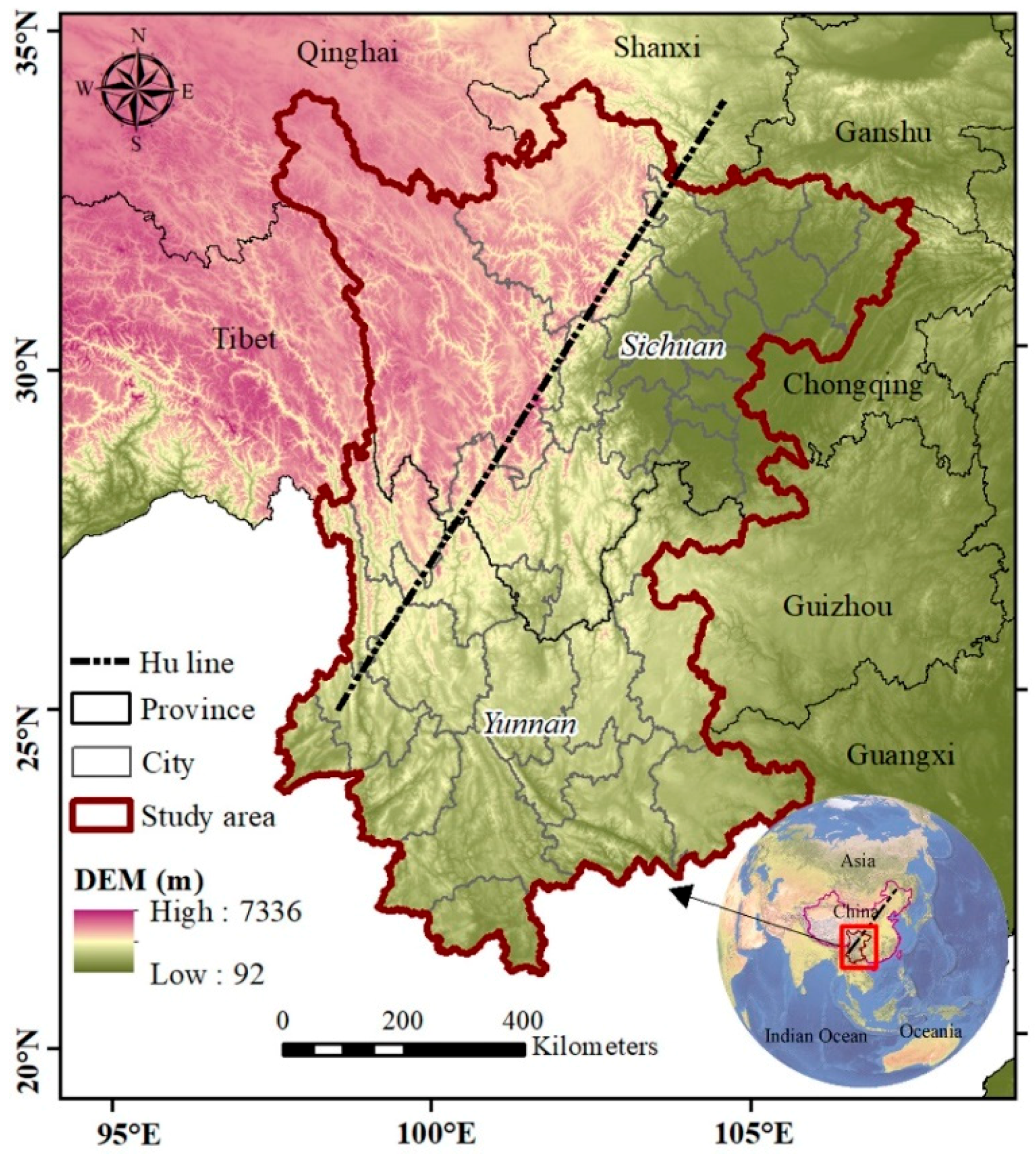
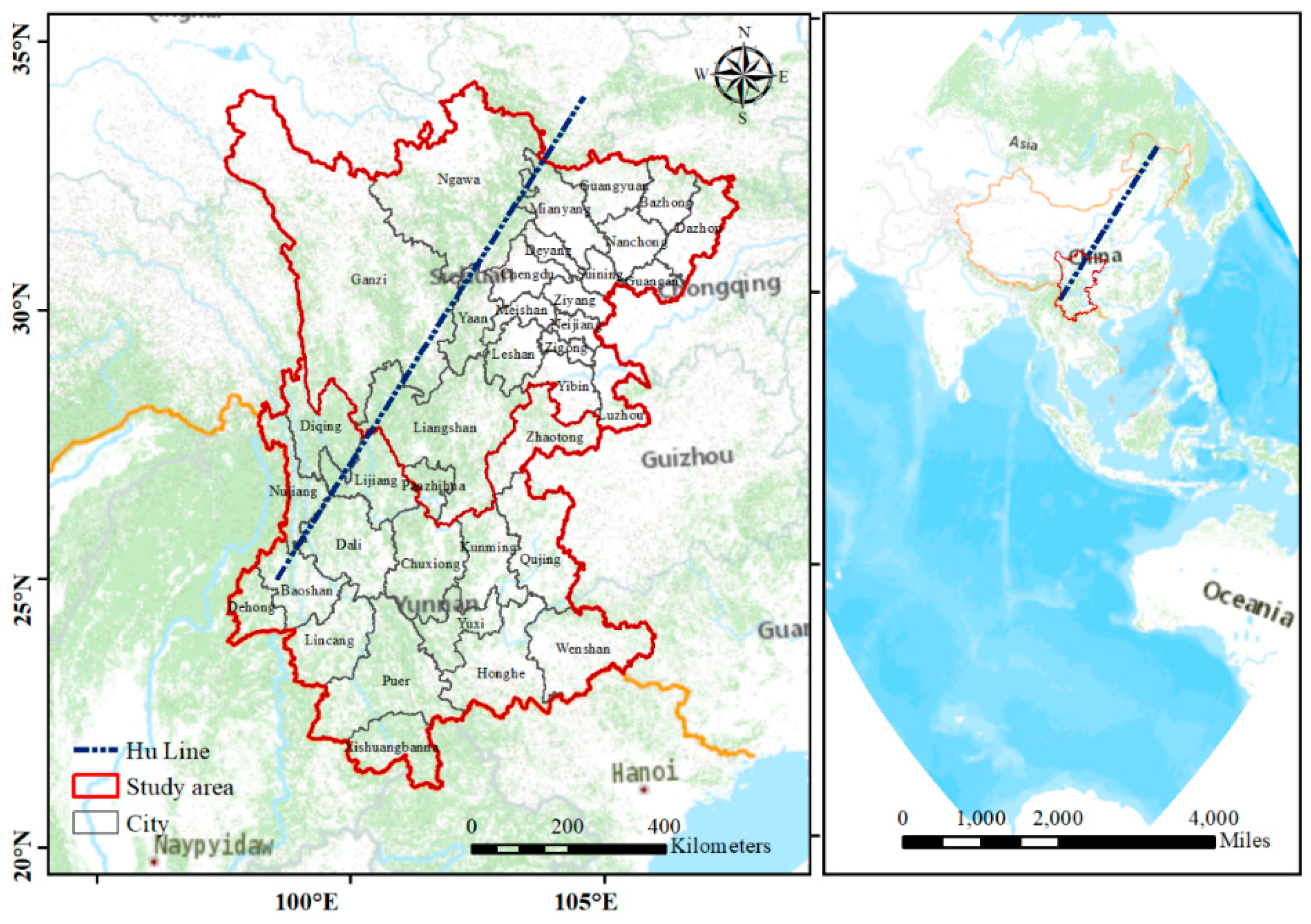
2.1. Study Area
2.2. Ecosystem Health Assessment Framework
2.3. Data Acquisition and Processing
2.3.1. Climate Change Index
2.3.2. Data Acquisition at the County Level
2.3.3. Comprehensive Assessment
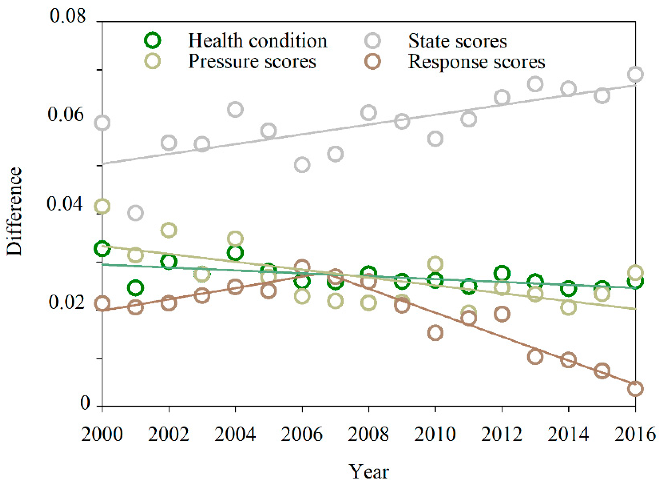
2.4. Analysis of Overall Evolution Characteristics
2.5. Analysis of Local Evolution Characteristics
3. Results
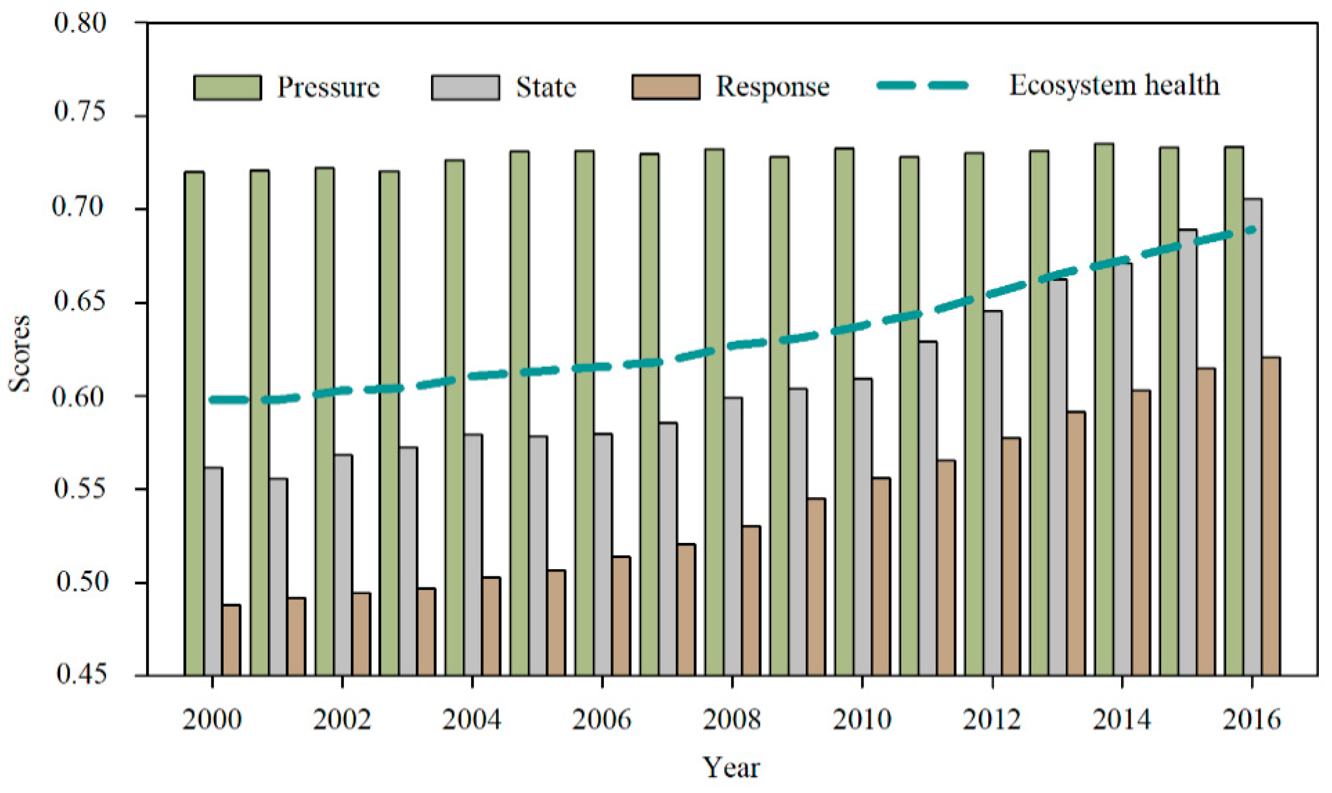
3.1. Global Features of Ecosystem Health Condition at the City Level in the Study Area
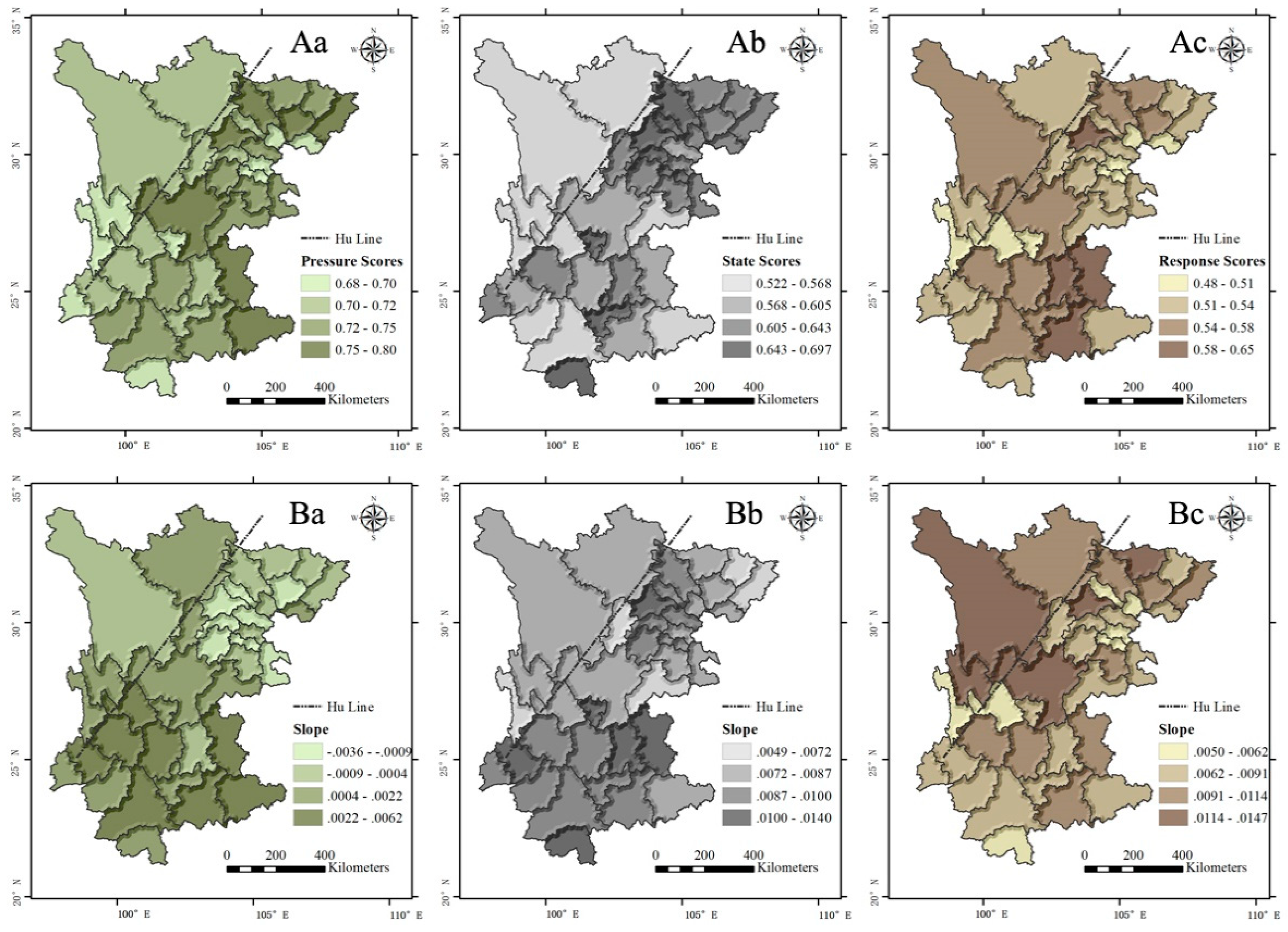
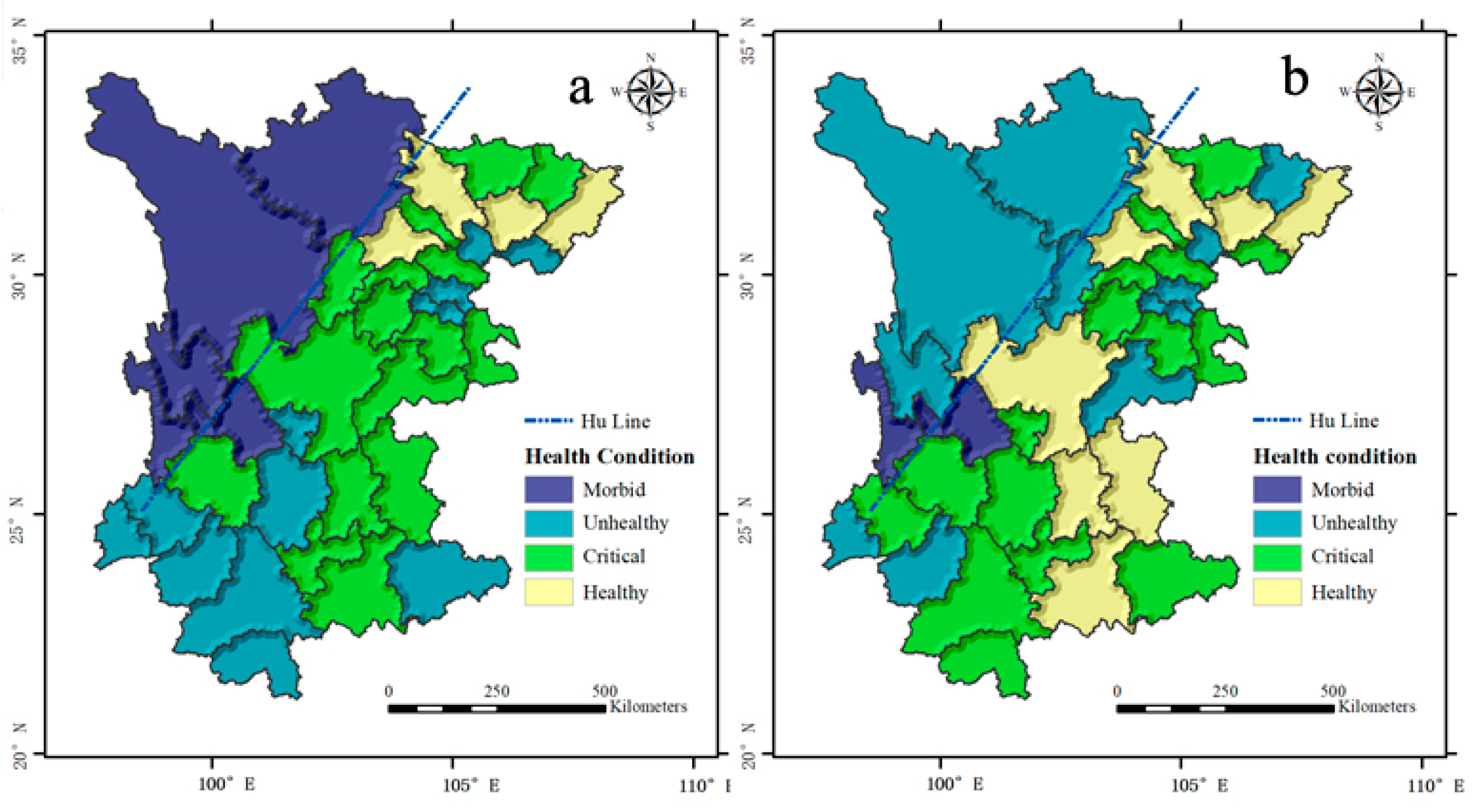
3.2. Spatio-Temporal Pattern Evolution of Ecosystem Health Condition at the City Level
3.2.1. Spatio-Temporal Pattern Evolution
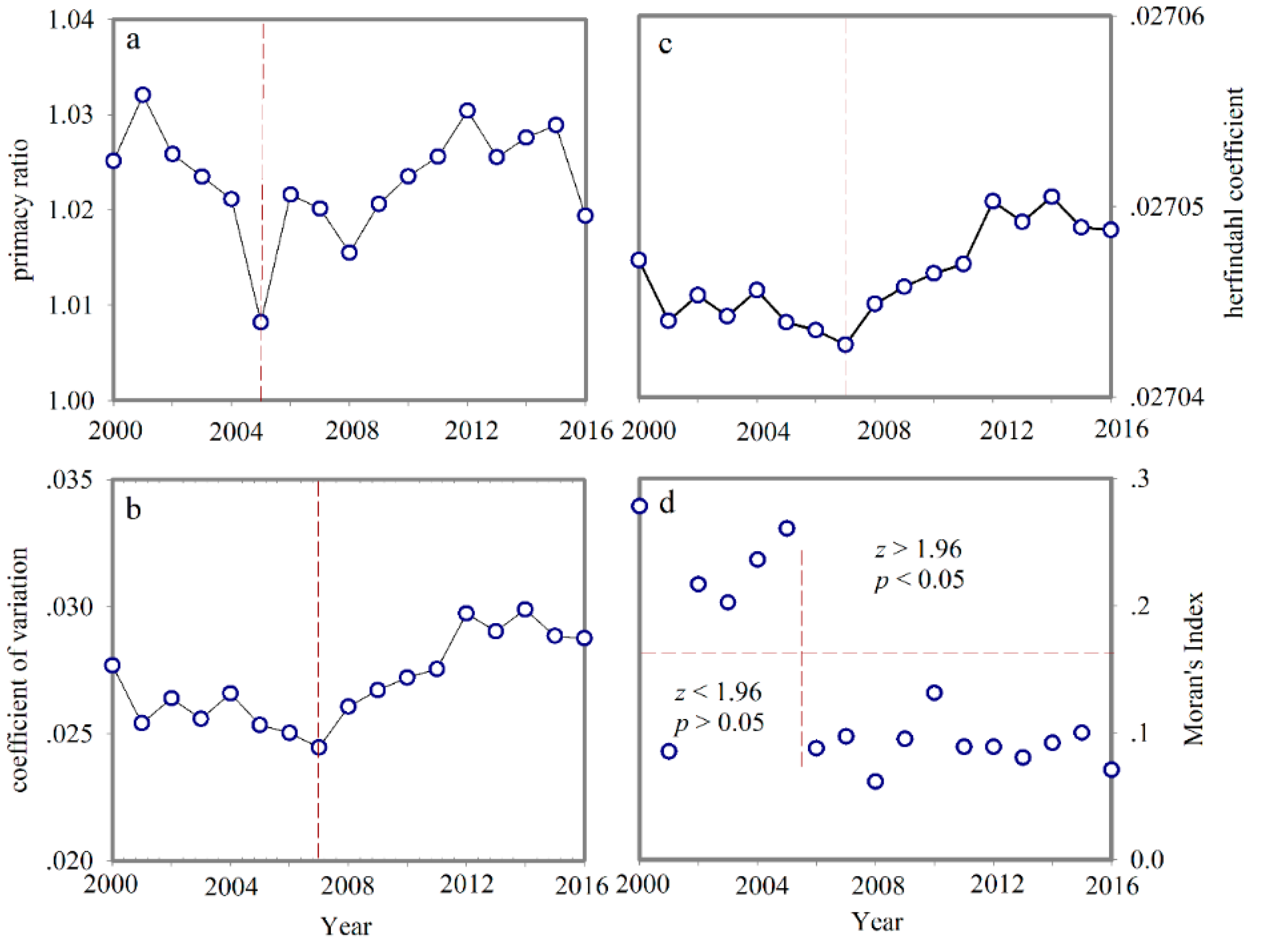
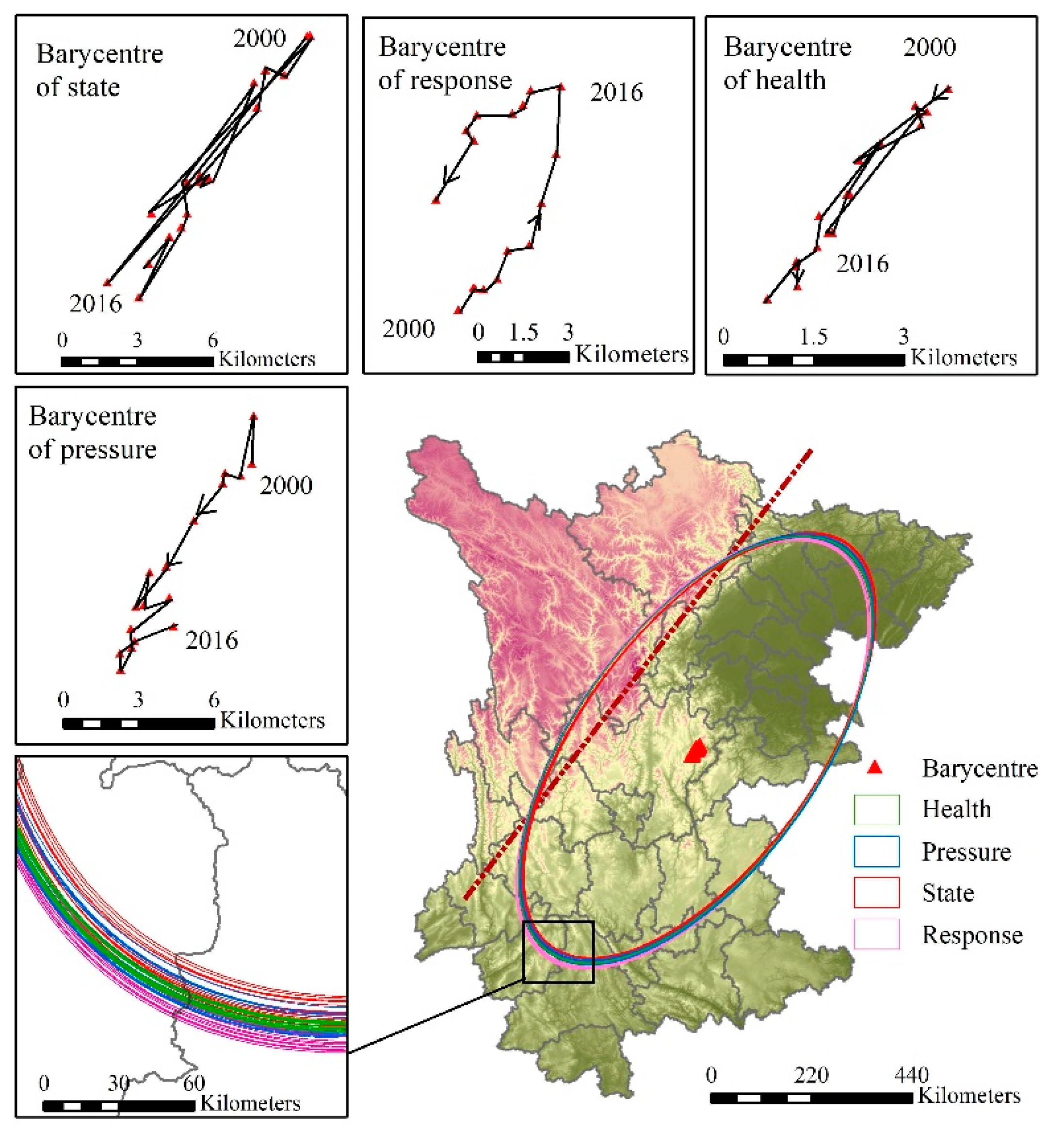
3.2.2. Results of the Spatial Gravity Center Model and Standard Deviation Ellipse
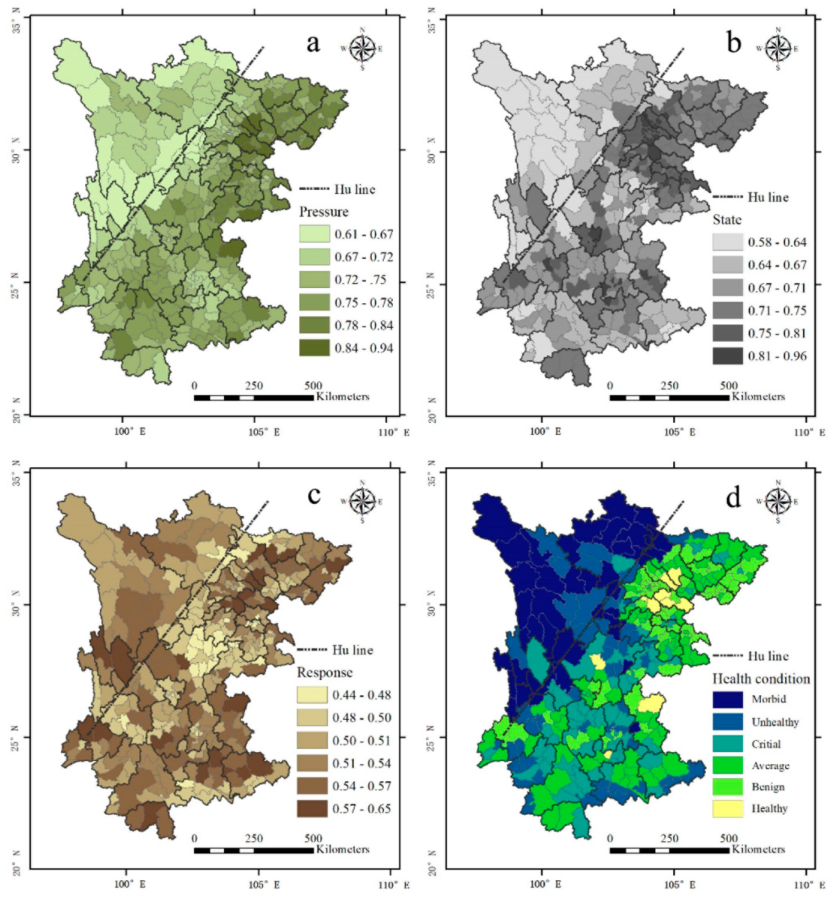
3.3. Ecosystem Health at the County Level in Sichuan and Yunnan
4. Discussion
4.1. Assessment Methodology
4.2. Dynamics of Ecosystem Health in Sichuan and Yunnan
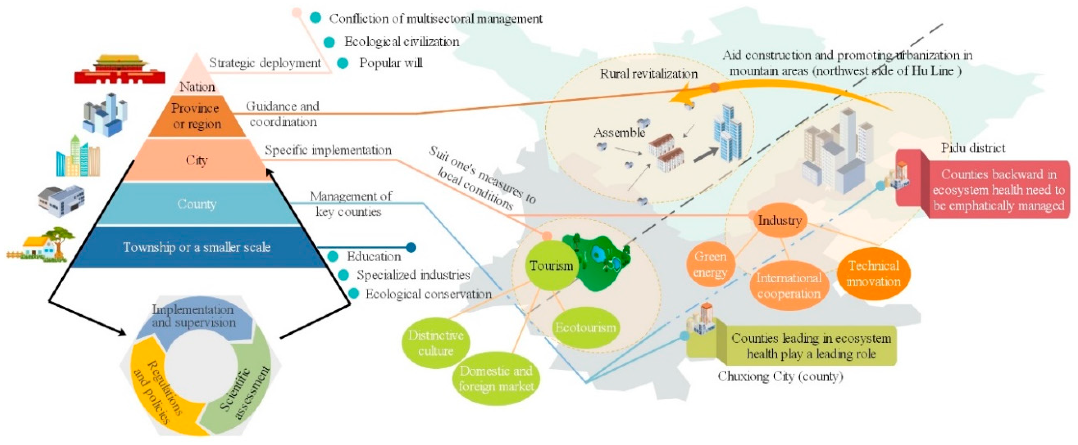
4.3. Suggestions and Implications
5. Conclusions
Author Contributions
Funding
Conflicts of Interest
Appendix A

Appendix B

| Province | City (Prefecture-Level City) | County | Pressure | State | Response | Healthy | Healthy Condition |
|---|---|---|---|---|---|---|---|
| Sichuan | Bazhong | Bazhou | 0.743 | 0.704 | 0.543 | 0.667 | Critical |
| Enyang | 0.76 | 0.694 | 0.533 | 0.667 | Critical | ||
| Nanjiang | 0.774 | 0.696 | 0.525 | 0.677 | Average | ||
| Pingchang | 0.769 | 0.688 | 0.561 | 0.683 | Average | ||
| Tongjiang | 0.783 | 0.691 | 0.512 | 0.678 | Average | ||
| Chengdu | Chenghua | 0.715 | 0.932 | 0.621 | 0.707 | Healthy | |
| Chongzhou | 0.742 | 0.778 | 0.562 | 0.699 | Benign | ||
| Dayi | 0.73 | 0.79 | 0.536 | 0.687 | Benign | ||
| Dujiangyan | 0.713 | 0.803 | 0.542 | 0.691 | Benign | ||
| Jinniu | 0.711 | 0.898 | 0.612 | 0.688 | Healthy | ||
| Jintang | 0.787 | 0.749 | 0.55 | 0.704 | Benign | ||
| Jinjiang | 0.715 | 0.942 | 0.638 | 0.714 | Healthy | ||
| Longquanyi | 0.727 | 0.888 | 0.511 | 0.722 | Healthy | ||
| Pengzhou | 0.732 | 0.804 | 0.558 | 0.708 | Benign | ||
| Pidu | 0.71 | 0.819 | 0.548 | 0.693 | Benign | ||
| Pujiang | 0.721 | 0.736 | 0.548 | 0.653 | Average | ||
| Qingbaijiang | 0.74 | 0.846 | 0.53 | 0.709 | Benign | ||
| Qingyang | 0.71 | 0.911 | 0.626 | 0.697 | Healthy | ||
| Qionglai | 0.746 | 0.779 | 0.566 | 0.699 | Benign | ||
| Shuangliu | 0.747 | 0.825 | 0.589 | 0.727 | Healthy | ||
| Wenjiang | 0.713 | 0.903 | 0.578 | 0.724 | Healthy | ||
| Wuhou | 0.71 | 0.851 | 0.612 | 0.668 | Healthy | ||
| Xindu | 0.739 | 0.85 | 0.557 | 0.719 | Healthy | ||
| Xinjin | 0.73 | 0.873 | 0.569 | 0.719 | Healthy | ||
| Dazhou | Dachuan | 0.799 | 0.721 | 0.543 | 0.704 | Benign | |
| Dazhu | 0.828 | 0.728 | 0.539 | 0.715 | Benign | ||
| Kaijiang | 0.761 | 0.722 | 0.527 | 0.673 | Average | ||
| Quxian | 0.831 | 0.693 | 0.535 | 0.708 | Benign | ||
| Tongchuan | 0.733 | 0.748 | 0.515 | 0.667 | Average | ||
| Wanyuan | 0.758 | 0.726 | 0.534 | 0.677 | Average | ||
| Xuanhan | 0.82 | 0.715 | 0.569 | 0.723 | Benign | ||
| Deyang | Guanghan | 0.755 | 0.82 | 0.542 | 0.709 | Benign | |
| Jingyang | 0.742 | 0.837 | 0.565 | 0.713 | Benign | ||
| Luojiang | 0.721 | 0.805 | 0.553 | 0.678 | Benign | ||
| Mianzhu | 0.731 | 0.805 | 0.542 | 0.693 | Benign | ||
| Shifang | 0.707 | 0.837 | 0.538 | 0.694 | Benign | ||
| Zhongjiang | 0.858 | 0.749 | 0.578 | 0.752 | Healthy | ||
| Ganzi | Batang | 0.65 | 0.637 | 0.52 | 0.598 | Morbid | |
| Baiyu | 0.677 | 0.625 | 0.482 | 0.604 | Morbid | ||
| Danba | 0.701 | 0.658 | 0.508 | 0.623 | Unhealthy | ||
| Daofu | 0.711 | 0.606 | 0.533 | 0.618 | Morbid | ||
| Daocheng | 0.612 | 0.631 | 0.588 | 0.601 | Morbid | ||
| Derong | 0.614 | 0.657 | 0.557 | 0.6 | Morbid | ||
| Dege | 0.672 | 0.595 | 0.475 | 0.593 | Morbid | ||
| Ganzi | 0.726 | 0.62 | 0.507 | 0.622 | Morbid | ||
| Jiulong | 0.663 | 0.701 | 0.489 | 0.624 | Morbid | ||
| Kangding | 0.667 | 0.665 | 0.523 | 0.625 | Morbid | ||
| Litang | 0.678 | 0.619 | 0.518 | 0.613 | Morbid | ||
| Luhuo | 0.734 | 0.615 | 0.516 | 0.625 | Unhealthy | ||
| Luding | 0.665 | 0.634 | 0.5 | 0.598 | Morbid | ||
| Seda | 0.713 | 0.607 | 0.537 | 0.627 | Morbid | ||
| Shiqu | 0.663 | 0.596 | 0.477 | 0.594 | Morbid | ||
| Xiangcheng | 0.63 | 0.653 | 0.542 | 0.601 | Morbid | ||
| Xinlong | 0.708 | 0.626 | 0.508 | 0.622 | Morbid | ||
| Yajiang | 0.68 | 0.638 | 0.563 | 0.629 | Unhealthy | ||
| Guang’an | Guangan | 0.787 | 0.731 | 0.574 | 0.7 | Benign | |
| Huaying | 0.758 | 0.741 | 0.533 | 0.677 | Average | ||
| Linshui | 0.83 | 0.715 | 0.552 | 0.71 | Benign | ||
| Qianfeng | 0.755 | 0.798 | 0.534 | 0.7 | Benign | ||
| Wusheng | 0.792 | 0.738 | 0.536 | 0.696 | Benign | ||
| Yuechi | 0.838 | 0.729 | 0.563 | 0.723 | Benign | ||
| Guangyuan | Cangxi | 0.783 | 0.722 | 0.617 | 0.712 | Benign | |
| Chaotian | 0.746 | 0.669 | 0.497 | 0.641 | Unhealthy | ||
| Jiange | 0.792 | 0.715 | 0.646 | 0.717 | Benign | ||
| Lizhou | 0.74 | 0.734 | 0.516 | 0.668 | Average | ||
| Qingchuan | 0.734 | 0.661 | 0.484 | 0.634 | Unhealthy | ||
| Wangcang | 0.754 | 0.728 | 0.505 | 0.672 | Average | ||
| Zhaohua | 0.749 | 0.71 | 0.522 | 0.657 | Critical | ||
| Leshan | Ebian | 0.722 | 0.656 | 0.493 | 0.628 | Unhealthy | |
| Emeishan | 0.729 | 0.745 | 0.552 | 0.672 | Average | ||
| Jiajiang | 0.731 | 0.733 | 0.571 | 0.672 | Average | ||
| Qianwei | 0.777 | 0.768 | 0.547 | 0.7 | Benign | ||
| Jinkouhe | 0.701 | 0.678 | 0.5 | 0.623 | Unhealthy | ||
| Jingyan | 0.776 | 0.729 | 0.582 | 0.681 | Benign | ||
| Shizhong | 0.745 | 0.777 | 0.546 | 0.689 | Benign | ||
| Mabian | 0.756 | 0.63 | 0.486 | 0.63 | Unhealthy | ||
| Muchuan | 0.762 | 0.688 | 0.513 | 0.652 | Critical | ||
| Shawan | 0.728 | 0.851 | 0.534 | 0.706 | Benign | ||
| Wutongqiao | 0.754 | 0.744 | 0.51 | 0.669 | Average | ||
| Liangshan | Butuo | 0.756 | 0.642 | 0.465 | 0.63 | Unhealthy | |
| Dechang | 0.753 | 0.747 | 0.534 | 0.674 | Average | ||
| Ganluo | 0.712 | 0.638 | 0.476 | 0.616 | Morbid | ||
| Huidong | 0.761 | 0.749 | 0.526 | 0.679 | Average | ||
| Huili | 0.774 | 0.772 | 0.573 | 0.706 | Benign | ||
| Jinyang | 0.737 | 0.625 | 0.471 | 0.618 | Morbid | ||
| Leibo | 0.763 | 0.674 | 0.483 | 0.649 | Critical | ||
| Meigu | 0.741 | 0.636 | 0.464 | 0.625 | Morbid | ||
| Mianning | 0.733 | 0.723 | 0.501 | 0.658 | Critical | ||
| Muli | 0.646 | 0.628 | 0.52 | 0.613 | Morbid | ||
| Ningnan | 0.739 | 0.716 | 0.534 | 0.653 | Critical | ||
| Puge | 0.761 | 0.646 | 0.489 | 0.637 | Unhealthy | ||
| Xichang | 0.789 | 0.79 | 0.613 | 0.733 | Healthy | ||
| Xide | 0.751 | 0.635 | 0.479 | 0.628 | Unhealthy | ||
| Yanyuan | 0.751 | 0.654 | 0.546 | 0.664 | Critical | ||
| Yuexi | 0.737 | 0.658 | 0.477 | 0.632 | Unhealthy | ||
| Zhaojue | 0.761 | 0.681 | 0.486 | 0.653 | Critical | ||
| Luzhou | Gulan | 0.818 | 0.638 | 0.504 | 0.672 | Critical | |
| Hejiang | 0.813 | 0.742 | 0.545 | 0.713 | Benign | ||
| Jiangyang | 0.733 | 0.839 | 0.541 | 0.704 | Benign | ||
| Longmatan | 0.713 | 0.822 | 0.549 | 0.686 | Benign | ||
| Luxian | 0.776 | 0.777 | 0.56 | 0.718 | Benign | ||
| Naxi | 0.742 | 0.765 | 0.539 | 0.674 | Average | ||
| Xuyong | 0.781 | 0.663 | 0.536 | 0.67 | Critical | ||
| Meishan | Danleng | 0.722 | 0.757 | 0.564 | 0.665 | Average | |
| Dongpo | 0.762 | 0.796 | 0.601 | 0.724 | Healthy | ||
| Hongya | 0.71 | 0.771 | 0.529 | 0.671 | Average | ||
| Pengshan | 0.932 | 0.728 | 0.572 | 0.744 | Healthy | ||
| Qingshen | 0.743 | 0.754 | 0.525 | 0.671 | Average | ||
| Renshou | 0.72 | 0.765 | 0.608 | 0.731 | Benign | ||
| Mianyang | Anzhou | 0.739 | 0.769 | 0.572 | 0.684 | Benign | |
| Beichuan | 0.704 | 0.647 | 0.475 | 0.613 | Morbid | ||
| Fucheng | 0.715 | 0.816 | 0.55 | 0.691 | Benign | ||
| Jiangyou | 0.746 | 0.777 | 0.616 | 0.714 | Benign | ||
| Pingwu | 0.718 | 0.626 | 0.474 | 0.614 | Morbid | ||
| Santai | 0.861 | 0.722 | 0.604 | 0.754 | Healthy | ||
| Yanting | 0.763 | 0.71 | 0.549 | 0.673 | Average | ||
| Youxian | 0.735 | 0.768 | 0.554 | 0.682 | Average | ||
| Zitong | 0.747 | 0.737 | 0.565 | 0.672 | Average | ||
| Nanchong | Gaoping | 0.77 | 0.72 | 0.502 | 0.672 | Average | |
| Jialing | 0.798 | 0.699 | 0.503 | 0.676 | Average | ||
| Langzhong | 0.776 | 0.725 | 0.548 | 0.691 | Average | ||
| Nanbu | 0.84 | 0.712 | 0.556 | 0.72 | Benign | ||
| Pengan | 0.774 | 0.726 | 0.528 | 0.682 | Average | ||
| Shunqing | 0.756 | 0.761 | 0.53 | 0.673 | Average | ||
| Xichong | 0.808 | 0.695 | 0.528 | 0.683 | Average | ||
| Yilong | 0.793 | 0.725 | 0.534 | 0.701 | Benign | ||
| Yingshan | 0.763 | 0.725 | 0.519 | 0.681 | Average | ||
| Neijiang | Dongxing | 0.764 | 0.719 | 0.511 | 0.673 | Average | |
| Longchang | 0.76 | 0.745 | 0.537 | 0.683 | Average | ||
| Shizhong | 0.737 | 0.729 | 0.503 | 0.658 | Critical | ||
| Weiyuan | 0.796 | 0.765 | 0.544 | 0.705 | Benign | ||
| Zizhong | 0.832 | 0.691 | 0.522 | 0.706 | Benign | ||
| Ngawa | Aba | 0.671 | 0.587 | 0.521 | 0.597 | Morbid | |
| Heishui | 0.707 | 0.654 | 0.496 | 0.622 | Morbid | ||
| Hongyuan | 0.679 | 0.673 | 0.511 | 0.622 | Morbid | ||
| Jinchuan | 0.723 | 0.655 | 0.527 | 0.635 | Unhealthy | ||
| Jiuzhaigou | 0.668 | 0.656 | 0.521 | 0.617 | Morbid | ||
| Lixian | 0.678 | 0.734 | 0.53 | 0.648 | Critical | ||
| Barkan | 0.722 | 0.661 | 0.547 | 0.644 | Unhealthy | ||
| Maoxian | 0.687 | 0.673 | 0.499 | 0.617 | Morbid | ||
| Rangtang | 0.715 | 0.604 | 0.535 | 0.62 | Morbid | ||
| Ruoergai | 0.638 | 0.649 | 0.499 | 0.596 | Morbid | ||
| Songpan | 0.679 | 0.66 | 0.515 | 0.623 | Morbid | ||
| Wenchuan | 0.671 | 0.717 | 0.484 | 0.631 | Unhealthy | ||
| Xiaojin | 0.685 | 0.625 | 0.526 | 0.61 | Morbid | ||
| Panzhihua | Dongqu | 0.695 | 0.902 | 0.512 | 0.685 | Benign | |
| Miyi | 0.728 | 0.814 | 0.538 | 0.694 | Benign | ||
| Renhe | 0.718 | 0.795 | 0.51 | 0.68 | Average | ||
| Xiqu | 0.698 | 0.844 | 0.528 | 0.656 | Benign | ||
| Yanbian | 0.736 | 0.751 | 0.525 | 0.672 | Average | ||
| Suining | Anju | 0.8 | 0.692 | 0.51 | 0.681 | Average | |
| Chuanshan | 0.749 | 0.741 | 0.543 | 0.667 | Average | ||
| Daying | 0.774 | 0.718 | 0.513 | 0.673 | Average | ||
| Pengxi | 0.786 | 0.714 | 0.512 | 0.68 | Average | ||
| Shehong | 0.818 | 0.724 | 0.516 | 0.702 | Benign | ||
| Yaan | Baoxing | 0.631 | 0.707 | 0.508 | 0.612 | Morbid | |
| Hanyuan | 0.683 | 0.66 | 0.517 | 0.618 | Morbid | ||
| Lushan | 0.668 | 0.725 | 0.52 | 0.634 | Unhealthy | ||
| Mingshan | 0.712 | 0.705 | 0.531 | 0.641 | Critical | ||
| Shimian | 0.677 | 0.739 | 0.497 | 0.64 | Unhealthy | ||
| Tianquan | 0.668 | 0.741 | 0.514 | 0.637 | Unhealthy | ||
| Yingjing | 0.626 | 0.722 | 0.504 | 0.617 | Morbid | ||
| Yucheng | 0.681 | 0.763 | 0.55 | 0.661 | Average | ||
| Yibin | Cuiping | 0.749 | 0.817 | 0.541 | 0.704 | Benign | |
| Gaoxian | 0.769 | 0.718 | 0.537 | 0.675 | Average | ||
| Zongxian | 0.758 | 0.717 | 0.526 | 0.665 | Average | ||
| Jiangan | 0.748 | 0.764 | 0.513 | 0.679 | Average | ||
| Junlian | 0.772 | 0.719 | 0.505 | 0.668 | Average | ||
| Nanxi | 0.739 | 0.772 | 0.589 | 0.69 | Benign | ||
| Pingshan | 0.772 | 0.675 | 0.53 | 0.655 | Critical | ||
| Xingwen | 0.758 | 0.721 | 0.517 | 0.67 | Average | ||
| Yibin | 0.823 | 0.74 | 0.52 | 0.714 | Benign | ||
| Changning | 0.752 | 0.762 | 0.554 | 0.683 | Benign | ||
| Zigong | Daan | 0.733 | 0.755 | 0.483 | 0.663 | Critical | |
| Fushun | 0.782 | 0.769 | 0.518 | 0.706 | Benign | ||
| Gongjing | 0.738 | 0.754 | 0.494 | 0.662 | Average | ||
| Rongxian | 0.81 | 0.747 | 0.548 | 0.71 | Benign | ||
| Yantan | 0.735 | 0.756 | 0.493 | 0.665 | Average | ||
| Ziliujing | 0.728 | 0.816 | 0.52 | 0.683 | Benign | ||
| Ziyang | Anyue | 0.889 | 0.705 | 0.604 | 0.755 | Healthy | |
| Jianyang | 0.922 | 0.695 | 0.6 | 0.761 | Healthy | ||
| Lezhi | 0.819 | 0.709 | 0.553 | 0.7 | Benign | ||
| Yanjiang | 0.878 | 0.72 | 0.567 | 0.735 | Healthy | ||
| Yunnan | Baoshan | Changning | 0.739 | 0.702 | 0.579 | 0.676 | Average |
| Longling | 0.706 | 0.684 | 0.529 | 0.642 | Unhealthy | ||
| Longyang | 0.738 | 0.761 | 0.569 | 0.711 | Benign | ||
| Shidian | 0.706 | 0.668 | 0.545 | 0.642 | Unhealthy | ||
| Tengchong | 0.769 | 0.695 | 0.579 | 0.697 | Average | ||
| Chuxiong | Chuxiong | 0.77 | 0.76 | 0.601 | 0.716 | Benign | |
| Dayao | 0.766 | 0.689 | 0.521 | 0.663 | Critical | ||
| Lufeng | 0.738 | 0.709 | 0.546 | 0.67 | Critical | ||
| Mouding | 0.751 | 0.667 | 0.499 | 0.644 | Unhealthy | ||
| Nanhua | 0.763 | 0.687 | 0.512 | 0.658 | Critical | ||
| Shuangbai | 0.759 | 0.666 | 0.554 | 0.658 | Critical | ||
| Wuding | 0.74 | 0.678 | 0.531 | 0.654 | Critical | ||
| Yaoan | 0.753 | 0.716 | 0.514 | 0.661 | Critical | ||
| Yongren | 0.739 | 0.685 | 0.532 | 0.647 | Critical | ||
| Yuanmou | 0.726 | 0.698 | 0.538 | 0.651 | Critical | ||
| Dali | Binchuan | 0.742 | 0.758 | 0.581 | 0.692 | Benign | |
| Dali | 0.738 | 0.811 | 0.569 | 0.714 | Benign | ||
| Eryuan | 0.729 | 0.743 | 0.514 | 0.67 | Average | ||
| Heqing | 0.734 | 0.694 | 0.521 | 0.653 | Critical | ||
| Jianchuan | 0.706 | 0.643 | 0.502 | 0.619 | Morbid | ||
| Midu | 0.756 | 0.757 | 0.506 | 0.682 | Average | ||
| Nanjian | 0.764 | 0.68 | 0.501 | 0.652 | Critical | ||
| Weishan | 0.752 | 0.682 | 0.503 | 0.653 | Critical | ||
| Xiangyun | 0.756 | 0.734 | 0.56 | 0.686 | Average | ||
| Yangbi | 0.728 | 0.684 | 0.507 | 0.636 | Unhealthy | ||
| Yongping | 0.719 | 0.684 | 0.512 | 0.633 | Unhealthy | ||
| Yunlong | 0.718 | 0.672 | 0.488 | 0.633 | Unhealthy | ||
| Dehong | Lianghe | 0.707 | 0.663 | 0.512 | 0.627 | Unhealthy | |
| Longchuan | 0.745 | 0.707 | 0.581 | 0.667 | Average | ||
| Mangxian | 0.734 | 0.702 | 0.585 | 0.676 | Average | ||
| Ruili | 0.747 | 0.743 | 0.595 | 0.68 | Benign | ||
| Yingjiang | 0.76 | 0.702 | 0.563 | 0.676 | Average | ||
| Diqing | Deqin | 0.622 | 0.673 | 0.612 | 0.634 | Unhealthy | |
| Weixi | 0.665 | 0.635 | 0.54 | 0.616 | Morbid | ||
| Shangri-la | 0.622 | 0.725 | 0.602 | 0.657 | Critical | ||
| Honghe | Gejiu | 0.74 | 0.727 | 0.548 | 0.671 | Average | |
| Hekou | 0.741 | 0.767 | 0.576 | 0.671 | Benign | ||
| Honghe | 0.73 | 0.668 | 0.483 | 0.637 | Unhealthy | ||
| Jianshui | 0.738 | 0.678 | 0.574 | 0.672 | Critical | ||
| Jinping | 0.749 | 0.657 | 0.486 | 0.644 | Unhealthy | ||
| Kaiyuan | 0.709 | 0.748 | 0.59 | 0.677 | Average | ||
| Luxi | 0.687 | 0.688 | 0.571 | 0.65 | Critical | ||
| Lvchun | 0.723 | 0.652 | 0.487 | 0.629 | Unhealthy | ||
| Mengzi | 0.764 | 0.681 | 0.574 | 0.674 | Average | ||
| Mile | 0.708 | 0.72 | 0.573 | 0.677 | Average | ||
| Pingbian | 0.762 | 0.642 | 0.504 | 0.64 | Unhealthy | ||
| Shiping | 0.75 | 0.679 | 0.539 | 0.66 | Critical | ||
| Yuanyang | 0.756 | 0.66 | 0.483 | 0.646 | Unhealthy | ||
| Kunming | Anning | 0.72 | 0.842 | 0.574 | 0.711 | Benign | |
| Chenggong | 0.683 | 0.738 | 0.55 | 0.658 | Critical | ||
| Dongchuan | 0.719 | 0.658 | 0.499 | 0.632 | Unhealthy | ||
| Fumin | 0.702 | 0.725 | 0.5 | 0.645 | Critical | ||
| Guandu | 0.688 | 0.868 | 0.582 | 0.704 | Benign | ||
| Jinning | 0.721 | 0.708 | 0.542 | 0.657 | Critical | ||
| Luquan | 0.754 | 0.667 | 0.542 | 0.665 | Critical | ||
| Panlong | 0.694 | 0.747 | 0.524 | 0.656 | Critical | ||
| Shilin | 0.688 | 0.687 | 0.548 | 0.638 | Unhealthy | ||
| Songming | 0.689 | 0.69 | 0.546 | 0.643 | Unhealthy | ||
| Wuhua | 0.691 | 0.861 | 0.5 | 0.697 | Benign | ||
| Xishan | 0.697 | 0.744 | 0.546 | 0.661 | Critical | ||
| Xundian | 0.739 | 0.646 | 0.522 | 0.647 | Unhealthy | ||
| Yiliang | 0.689 | 0.726 | 0.537 | 0.656 | Critical | ||
| Lijiang | Gucheng | 0.689 | 0.718 | 0.554 | 0.648 | Critical | |
| Huaping | 0.73 | 0.65 | 0.518 | 0.632 | Unhealthy | ||
| Ninglango | 0.687 | 0.589 | 0.492 | 0.6 | Morbid | ||
| Yongsheng | 0.748 | 0.669 | 0.534 | 0.661 | Critical | ||
| Yulong | 0.678 | 0.647 | 0.529 | 0.62 | Morbid | ||
| Cangyuan | 0.751 | 0.648 | 0.524 | 0.641 | Unhealthy | ||
| Fengqing | 0.757 | 0.656 | 0.523 | 0.655 | Critical | ||
| Gengma | 0.739 | 0.692 | 0.567 | 0.662 | Critical | ||
| Linxiang | 0.752 | 0.675 | 0.526 | 0.656 | Critical | ||
| Shuangjiang | 0.746 | 0.642 | 0.526 | 0.638 | Unhealthy | ||
| Yongde | 0.745 | 0.627 | 0.539 | 0.643 | Unhealthy | ||
| Yunxian | 0.788 | 0.654 | 0.52 | 0.667 | Critical | ||
| Zhenkang | 0.722 | 0.632 | 0.532 | 0.628 | Unhealthy | ||
| Nujiang | Fugong | 0.67 | 0.607 | 0.497 | 0.595 | Morbid | |
| Gongshan | 0.64 | 0.633 | 0.533 | 0.599 | Morbid | ||
| Lanping | 0.707 | 0.615 | 0.507 | 0.615 | Morbid | ||
| Lushui | 0.708 | 0.628 | 0.503 | 0.617 | Morbid | ||
| Puer | Jiangcheng | 0.72 | 0.656 | 0.514 | 0.628 | Unhealthy | |
| Jingdong | 0.788 | 0.664 | 0.53 | 0.672 | Critical | ||
| Jinggu | 0.78 | 0.692 | 0.537 | 0.68 | Average | ||
| Lancang | 0.809 | 0.621 | 0.531 | 0.678 | Critical | ||
| Menglian | 0.742 | 0.66 | 0.531 | 0.638 | Critical | ||
| Mojiang | 0.765 | 0.638 | 0.519 | 0.653 | Unhealthy | ||
| Ninger | 0.754 | 0.656 | 0.528 | 0.649 | Critical | ||
| Simao | 0.74 | 0.705 | 0.543 | 0.656 | Critical | ||
| Ximeng | 0.756 | 0.617 | 0.516 | 0.633 | Unhealthy | ||
| Zhenyuan | 0.771 | 0.663 | 0.537 | 0.659 | Critical | ||
| Qujing | Fuyuan | 0.753 | 0.706 | 0.508 | 0.674 | Critical | |
| Huize | 0.828 | 0.665 | 0.505 | 0.696 | Average | ||
| Luliang | 0.718 | 0.706 | 0.558 | 0.672 | Critical | ||
| Luoping | 0.718 | 0.74 | 0.536 | 0.68 | Average | ||
| Malong | 0.702 | 0.639 | 0.524 | 0.621 | Unhealthy | ||
| Qilin | 0.717 | 0.809 | 0.569 | 0.708 | Benign | ||
| Shizong | 0.692 | 0.71 | 0.532 | 0.653 | Critical | ||
| Xuanwei | 0.945 | 0.66 | 0.613 | 0.774 | Healthy | ||
| Zhanyi | 0.775 | 0.715 | 0.55 | 0.688 | Average | ||
| Wenshan | Funing | 0.722 | 0.647 | 0.499 | 0.636 | Unhealthy | |
| Guangnan | 0.793 | 0.625 | 0.543 | 0.679 | Critical | ||
| Malipo | 0.742 | 0.628 | 0.508 | 0.632 | Unhealthy | ||
| Maguan | 0.784 | 0.641 | 0.514 | 0.656 | Critical | ||
| Qiubei | 0.751 | 0.631 | 0.524 | 0.65 | Unhealthy | ||
| Wenshan | 0.765 | 0.685 | 0.544 | 0.673 | Average | ||
| Xichou | 0.738 | 0.623 | 0.509 | 0.626 | Unhealthy | ||
| Yanshan | 0.773 | 0.65 | 0.598 | 0.683 | Average | ||
| Xishuangbanna | Jinghong | 0.725 | 0.754 | 0.572 | 0.687 | Average | |
| Menghai | 0.74 | 0.739 | 0.552 | 0.686 | Average | ||
| Mengla | 0.682 | 0.746 | 0.552 | 0.651 | Critical | ||
| Yuxi | Chengjiang | 0.688 | 0.741 | 0.535 | 0.654 | Critical | |
| Eshan | 0.747 | 0.746 | 0.57 | 0.686 | Benign | ||
| Hongta | 0.737 | 0.938 | 0.504 | 0.75 | Healthy | ||
| Huaning | 0.691 | 0.72 | 0.553 | 0.65 | Critical | ||
| Jiangchuan | 0.702 | 0.748 | 0.523 | 0.662 | Critical | ||
| Tonghai | 0.71 | 0.713 | 0.573 | 0.663 | Critical | ||
| Xinping | 0.761 | 0.73 | 0.549 | 0.687 | Average | ||
| Yimen | 0.749 | 0.725 | 0.52 | 0.667 | Average | ||
| Yuanjiang | 0.753 | 0.717 | 0.525 | 0.667 | Average | ||
| Zhaotong | Daguan | 0.782 | 0.617 | 0.494 | 0.642 | Unhealthy | |
| Ludian | 0.766 | 0.644 | 0.526 | 0.653 | Critical | ||
| Qiaojia | 0.778 | 0.657 | 0.498 | 0.66 | Critical | ||
| Shuifu | 0.751 | 0.708 | 0.476 | 0.652 | Critical | ||
| Suijiang | 0.749 | 0.639 | 0.498 | 0.632 | Unhealthy | ||
| Weixin | 0.793 | 0.641 | 0.486 | 0.653 | Critical | ||
| Yanjin | 0.786 | 0.636 | 0.496 | 0.651 | Critical | ||
| Yiliang | 0.773 | 0.666 | 0.488 | 0.659 | Critical | ||
| Yongshan | 0.796 | 0.642 | 0.49 | 0.658 | Critical | ||
| Zhaoyang | 0.794 | 0.715 | 0.54 | 0.699 | Average | ||
| Zhenxiong | 0.89 | 0.622 | 0.524 | 0.707 | Benign |
References
- Peng, J.; Liu, Y.; Li, T.; Wu, J. Regional ecosystem health response to rural land use change: A case study in Lijiang City, China. Ecol. Indic. 2017, 2017, 399–410. [Google Scholar] [CrossRef]
- Manzoor, S.A.; Malik, A.; Zubair, M.; Griffiths, G.H.; Lukac, M. Linking Social Perception and Provision of Ecosystem Services in a Sprawling Urban Landscape: A Case Study of Multan, Pakistan. Sustainability 2019, 11, 654. [Google Scholar] [CrossRef]
- Zoomers, A.; Noorloos, F.V.; Otsuki, K.; Stee, G.; Westen, G. The Rush for Land in an Urbanizing World: From Land Grabbing Toward Developing Safe, Resilient, and Sustainable Cities and Landscapes. World Dev. 2017, 92, 242–252. [Google Scholar] [CrossRef]
- Torres, R.; Gasparri, N.I.; Blendinger, P.G.; Grau, H.R. Land-use and land-cover effects on regional biodiversity distribution in a subtropical dry forest: A hierarchical integrative multi-taxa study. Reg. Environ. Chang. 2014, 14, 1549–1561. [Google Scholar] [CrossRef]
- Cano-Ortiz, A.; Fuentes, J.C.P.; Gomes, C.J.P.; Musarella, C.M.; Cano, E. Expansion of the juniperus genus due to anthropic activity. In Old-Growth Forest and Coniferous Forests; Weber, R.P., Ed.; Nova Science Publishers: New York, NY, USA, 2015; pp. 55–65. [Google Scholar]
- Cano, E.; Musarella, C.M.; Cano-Ortiz, A.; Fuentes, J.C.P.; Spampinato, G. Geobotanical Study of the Microforests of Juniperus oxycedrus subsp. badia in the Central and Southern Iberian Peninsula. Sustainability 2019, 11, 1111. [Google Scholar] [CrossRef]
- Costanza, R. Ecosystem health and ecological engineering. Ecol. Eng. 2012, 45, 24–29. [Google Scholar] [CrossRef]
- Sun, T.; Lin, W.; Chen, G.; Guo, P.; Ying, Z. Wetland ecosystem health assessment through integrating remote sensing and inventory data with an assessment model for the Hangzhou Bay, China. Sci. Total Environ. 2016, 566, 627–640. [Google Scholar] [CrossRef]
- Hauser, M. Nature versus Nuture Redux. Science 2002, 298, 1554–1555. [Google Scholar] [CrossRef]
- Mariano, D.A.; Santos, C.A.C.D.; Wardlow, B.D.; Anderson, M.C.; Schiltmeyer, A.V.; Tadesse, T.; Svoboda, M.D. Use of remote sensing indicators to assess effects of drought and human-induced land degradation on ecosystem health in Northeastern Brazil. Remote Sens. Environ. 2018, 213, 129–143. [Google Scholar] [CrossRef]
- Rapport, D.J. The ecology of health. Ecology 2012, 93, 1241–1242. [Google Scholar]
- Su, S.; Zhang, Z.; Xiao, R.; Jiang, Z.; Chen, T.; Zhang, L.; Wu, J. Geospatial assessment of agroecosystem health: Development of an integrated index based on catastrophe theory. Stoch. Environ. Res. Risk Assess. 2012, 26, 321–334. [Google Scholar] [CrossRef]
- Fisher, M.C.; Henk, D.A.; Briggs, C.J.; Brownstein, J.S.; Madoff, L.C.; Mccraw, S.L.; Gurr, S.J. Emerging fungal threats to animal, plant and ecosystem health. Nature 2012, 484, 186–194. [Google Scholar] [CrossRef] [PubMed]
- Wu, N.; Liu, A.; Wang, Y.; Li, L.; Chao, L.; Liu, G. An Assessment Framework for Grassland Ecosystem Health with Consideration of Natural Succession: A Case Study in Bayinxile, China. Sustainability 2019, 11, 1096. [Google Scholar] [CrossRef]
- Xu, F.L.; Lam, K.C.; Zhao, Z.Y.; Zhan, W.; Chen, Y.D.; Tao, S. Marine coastal ecosystem health assessment: A case study of the Tolo Harbour, Hong Kong, China. Ecol. Model. 2004, 173, 355–370. [Google Scholar] [CrossRef]
- Su, M.; Yang, Z.; Chen, B.; Ulgiati, S. Urban ecosystem health assessment based on emergy and set pair analysis—A comparative study of typical Chinese cities. Ecol. Model. 2009, 220, 2341–2348. [Google Scholar] [CrossRef]
- Jia, R.Y.; Liu, X.; Zhao, X.G.; Song, S. Assessment of ecosystem health in Shenfu mining area. Coal Geology. 2011, 39, 46–51. [Google Scholar]
- Rapport, D.J. Ecosystem Health: Exploring the Territory; University of Guelph: Guelph, ON, Canada, 1995; Volume 1, pp. 5–13. [Google Scholar]
- Ogden, J.C.; Baldwin, J.D.; Bass, O.L.; Browder, J.A.; Cook, M.I.; Frederick, P.E.; Frezza, P.C.; Galvez, R.A.; Hodgson, A.B.; Meyer, K.D.; et al. Waterbirds as indicators of ecosystem health in the coastal marine habitats of southern Florida: 1. Selection and justification for a suite of indicator species. Ecol. Indic. 2014, 44, 148–163. [Google Scholar] [CrossRef]
- Colin, N.; Porte, C.; Fernandes, D.; Barata, C.; Padrós, F.; Carrassón, M.; Monroy, M.; Cano-Rocabayera, O.; Sostoa, A.D.; Piña, B.; et al. Ecological relevance of biomarkers in monitoring studies of macro-invertebrates and fish in Mediterranean rivers. Sci. Total Environ. 2015, 540, 307–323. [Google Scholar] [CrossRef]
- Merlo, M.E.; Garrido-Becerra, J.A.; Mota, J.F.; Salmerón-Sánchez, E.; Martínez-Hernández, F.; Mendoza-Fernández, A.; Pérez-García, F.J. Threshold ionic contents for defining the nutritional strategies of gypsophile flora. Ecol. Indic. 2019, 97, 247–259. [Google Scholar] [CrossRef]
- Bai, X.; Tang, J. Ecological security assessment of Tianjin by PSR model. Procedia Environ. Sci. 2010, 2, 881–887. [Google Scholar] [CrossRef]
- Patrick, D.L.; Bush, J.W.; Chen, M.M. Toward an Operational Definition of Health. J. Health Soc. Behav. 1973, 14, 6–23. [Google Scholar] [CrossRef] [PubMed]
- Su, M.; Fath, B.D.; Yang, Z.; Chen, B.; Liu, G. Ecosystem health pattern analysis of urban clusters based on emergy synthesis: Results and implication for management. Energy Policy 2013, 59, 600–613. [Google Scholar] [CrossRef]
- Chen, Z.; Yin, Q.; Li, L.; Xu, H. Ecosystem health assessment by using remote sensing derived data: A case study of terrestrial region along the coast in Zhejiang province. In Proceedings of the 2010 IEEE International Geoscience and Remote Sensing Symposium, Honolulu, HI, USA, 25–30 July 2010. [Google Scholar]
- Liu, D.; Hao, S. Ecosystem Health Assessment at County-Scale Using the Pressure-State-Response Framework on the Loess Plateau, China. Int. J. Environ. Res. Public Health 2017, 14, 2. [Google Scholar] [CrossRef] [PubMed]
- Yu, G.; Yu, Q.; Hu, L.; Zhang, S.; Fu, T.; Zhou, X.; He, X.; Liu, Y.; Wang, S.; Jia, H. Ecosystem health assessment based on analysis of a land use database. Appl. Geogr. 2013, 44, 154–164. [Google Scholar] [CrossRef]
- Deng, X.; Bai, X. Sustainable Urbanization in Western China. Environ. Sci. Policy Sustain. Dev. 2014, 56, 12–24. [Google Scholar] [CrossRef]
- Hu, H. The distribution of population in China, with statistics and maps. Acta Geogr. Sin. 1935, 15, 1–24. [Google Scholar]
- Li, S.; Zhao, Z.; Wang, Y. Urbanization process and effects of natural resource and environment in China: Research trends and future directions. Prog. Geogr. 2009, 28, 63–70. [Google Scholar]
- Zhao, M.; Liu, S.; Liu, Z.; Qi, W. China’s different spatial patterns of population growth based on the “Hu Line”. J. Geogr. Sci. 2016, 26, 1611–1625. [Google Scholar]
- Peng, L.; Deng, W.; Zhang, H.; Sun, J.; Xiong, J. Focus on economy or ecology? A three-dimensional trade-off based on ecological carrying capacity in southwest China. Nat. Resource Model. 2018, 32, e12201. [Google Scholar] [CrossRef]
- Olson, D.M.; Dinerstein, E. The global 200: Priority ecoregions for global conservation. Ann. Mo. Bot. Gard. 2002, 89, 199–224. [Google Scholar] [CrossRef]
- Xu, J.; Wilkes, A. Conservation, Biodiversity impact analysis in northwest Yunnan, southwest China. Biodivers. Conserv. 2004, 13, 959–983. [Google Scholar] [CrossRef]
- Zhang, H.; Sun, J.; Xiong, J. Spatial-temporal patterns and controls of evapotranspiration across the Tibetan Plateau (2000–2012). Adv. Meteorol. 2017, 2017, 12. [Google Scholar] [CrossRef]
- Xiong, J.; Ye, C.; Cheng, W.; Guo, L.; Zhou, C.; Zhang, X. The Spatiotemporal Distribution of Flash Floods and Analysis of Partition Driving Forces in Yunnan Province. Sustainability 2019, 11, 2926. [Google Scholar] [CrossRef]
- Rapport, D.J.; Singh, A. An EcoHealth-based framework for state of environment reporting. Ecol. Indic. 2006, 6, 409–428. [Google Scholar] [CrossRef]
- Rapport, D.J.; Regier, H.A.; Hutchinson, T.C. Ecosystem behavior under stress. Am. Nat. 1985, 125, 617–640. [Google Scholar] [CrossRef]
- Ehrenfeld, D.; Costanza, R.; Norton, B.G.; Haskell, B.D. Ecosystem Health: New Goals for Environmental Management; Norton, B.G., Costanza, R., Haskell, B., Eds.; Island Press: Solomons, MD, USA, 1992. [Google Scholar]
- Hua, Y.; Yan, M.; Limin, D. Land ecological security assessment for Bai Autonomous Prefecture of Dali based using PSR model--with data in 2009 as case. Energy Procedia 2011, 5, 2172–2177. [Google Scholar] [CrossRef]
- Burkhard, B.; Müller, F. Drivers-Pressure-State-Impact-Response; Jorgensen, S.E., Fath, B.D., Eds.; Elsevier: Oxford, UK, 2008; pp. 967–970. [Google Scholar] [CrossRef]
- Thomas, C.D.; Cameron, A.; Green, R.E.; Bakkenes, M.; Beaumont, L.J.; Collingham, Y.C.; Erasmus, B.F.N.; De Siqueira, M.F.; Grainger, A.; Hannah, L.; et al. Extinction risk from climate change. Nature 2004, 427, 145–148. [Google Scholar] [CrossRef] [PubMed]
- Ding, M.; Heiser, M.; Hübl, J.; Fuchs, S. Regional vulnerability assessment for debris flows in China—A CWS approach. Landslides 2016, 13, 537–550. [Google Scholar] [CrossRef]
- Kouli, M.; Loupasakis, C.; Soupios, P.; Vallianatos, F. Landslide hazard zonation in high risk areas of Rethymno Prefecture, Crete Island, Greece. Nat. Hazards 2010, 52, 599–621. [Google Scholar] [CrossRef]
- Yang, S.E.; Wu, B.F. Calculation of monthly precipitation anomaly percentage using web-serviced remote sensing data. In Proceedings of the 2010 2nd International Conference on Advanced Computer Control, Shenyang, China, 27–29 March 2010. [Google Scholar]
- van Vuuren, D.P.; Smith, S.J.; Riahi, K. Downscaling socioeconomic and emissions scenarios for global environmental change research: A review. Clim. Chang. 2010, 1, 393–404. [Google Scholar] [CrossRef]
- Immerzeel, W.W.; Rutten, M.M.; Droogers, P. Spatial downscaling of TRMM precipitation using vegetative response on the Iberian Peninsula. Remote Sens. Environ. 2009, 113, 362–370. [Google Scholar] [CrossRef]
- Azaele, S.; Cornell, S.J.; Kunin, W.E. Downscaling species occupancy from coarse spatial scales. Ecol. Appl. 2012, 22, 1004–1014. [Google Scholar] [CrossRef] [PubMed]
- Jin, Y.; Lu, Z.; Tan, F.; Zhang, M.; Zhang, H. Assessment of ecological carrying capacity on the typical resources-based cities: A case study of Tangshan City. Acta Ecol. Sin. 2015, 35, 4852–4859. [Google Scholar]
- Xiong, J.; Sun, M.; Zhang, H.; Cheng, W.; Yang, Y.; Sun, M.; Cao, Y.; Wang, J. A neural network model of optimal scheduling system of public utility buses in Epifanio Delos Santos Avenue (EDSA). Nat. Hazards Earth Syst. 2019, 2019, 629–653. [Google Scholar] [CrossRef]
- Jin, C.; Xu, J.; Lu, Y. Study on disparity of tourism scale for cities in Yangtze-Delta and construction for the system of rank-size distribution. Economic Geography. Econ. Geogr. 2007, 04, 676–680. [Google Scholar]
- Zhou, L.; Zhou, C.; Yang, F.; Wang, B.; Sun, D. Spatio-temporal evolution and the influencing factors of PM_(2.5) in China between 2000 and 2011. Acta Geogr. Sin. 2017, 29, 253–270. [Google Scholar] [CrossRef]
- Xin, H.E.; Jiang, G.H.; Zhang, R.J.; Wen-Qiu, M.A.; Zhou, T. Temporal and Spatial Variation of Land Ecosystem Health Based on the Pressure-State-Response Model: A Case Study of Pinggu District, Beijing. J. Nat. Resour. 2015, 30, 2057–2068. [Google Scholar]
- He, Y.; Chen, Y.; Tang, H.; Yao, Y.; Yang, P.; Chen, Z. Exploring spatial change and gravity center movement for ecosystem services value using a spatially explicit ecosystem services value index and gravity model. Environ. Monit. Assess. 2011, 175, 563–571. [Google Scholar] [CrossRef]
- Wen, J.; Pu, L.; Li, S. The spatial-temporal changes of the ecosystem service value by land use and land cover change in Circum-Taihu Lake region. In Proceedings of the 2010 18th International Conference on Geoinformatics, Beijing, China, 18–20 June 2010. [Google Scholar]
- Chen, J.; Yang, S.T.; Li, H.W.; Zhang, B.; Lv, J.R. Research on Geographical Environment Unit Division Based on the Method of Natural Breaks (Jenks). ISPRS Int. Arch. Photogramm. Remote Sens. 2013, XL-4/W3(4), 47–50. [Google Scholar] [CrossRef]
- Taramelli, A.; Melelli, L.; Pasqui, M.; Sorichetta, A. Modelling risk hurricane elements in potentially affected areas by a GIS system. Nat. Hazards Risk 2010, 1, 349–373. [Google Scholar] [CrossRef]
- Rapport, D.J. Eco-cultural health, global health, and sustainability. Ecol. Res. 2011, 26, 1039–1049. [Google Scholar] [CrossRef]
- Frashure, K.M.; Bowen, R.E.; Chen, R.F. An integrative management protocol for connecting human priorities with ecosystem health in the Neponset River Estuary. Ocean Coast. Manag. 2012, 69, 255–264. [Google Scholar] [CrossRef]
- Dereynier, Y.L.; Levin, P.S.; Shoji, N.L. Bringing stakeholders, scientists, and managers together through an integrated ecosystem assessment process. Mar. Policy 2010, 34, 534–540. [Google Scholar] [CrossRef]
- Lin, Y.C.; Huang, S.L.; Budd, W.W. Assessing the environmental impacts of high-altitude agriculture in Taiwan: A Driver-Pressure-State-Impact-Response (DPSIR) framework and spatial emergy synthesis. Ecol. Indic. 2013, 32, 42–50. [Google Scholar] [CrossRef]
- Sekovskia, I.; Dennison, W.C. Megacities in the coastal zone: Using a driver-pressure-state-impact-response framework to address complex environmental problems. Estuar. Coast. Shelf Sci. 2012, 96, 48–59. [Google Scholar] [CrossRef]
- Wang, X.; Zhong, X.; Gao, P. A GIS-based decision support system for regional eco-security assessment and its application on the Tibetan Plateau. J. Environ. Manag. 2010, 91, 1981–1990. [Google Scholar]
- Liu, Y. Study on the agricultural water and land carrying capacity in sichuan province. In Chinese Academy of Agricultural Sciences; Chinese Academy of Agricultural Sciences: Beijing, China, 2010. [Google Scholar]
- Hong, H.; Liao, H.; Wei, C.; Li, T. Health assessment of a land use system used in the ecologically sensitive area of the Three Gorges reservoir area, based on the improved TOPSIS Method. Acta Ecol. Sin. 2015, 35, 8016–8027. [Google Scholar]
- Pettorelli, N.; Vik, J.O.; Mysterud, A.; Gaillard, J.M.; Tucker, C.J.; Stenseth, N.C.; Stenseth, N.C. Using the satellite-derived NDVI to assess ecological responses to environmental change. Trends Ecol. Evol. 2005, 20, 503–510. [Google Scholar] [CrossRef]
- Hui, F.; Liu, X.; Sun, Y. The Application of RS in Wetland Ecosystem Health Assessment: A Case Study of Dagu River Estuary. In Proceedings of the 2008 International Workshop on Education Technology and Training & 2008 International Workshop on Geoscience and Remote Sensing, Shanghai, China, 21–22 December 2009. [Google Scholar]
- Hao, S.; Chen, N. Analysis of Land-Use Changes in Loess Hilly Region Based on PSR Model: A Case Study in Shanghuang Study Area in GuYuan City. In Proceedings of the International Conference on Bioinformatics & Biomedical Engineering, Chengdu, China, 18–20 June 2010. [Google Scholar]
- Wu, W.; Xu, Z.; Zhan, C.; Yin, X.; Yu, S. A new framework to evaluate ecosystem health: A case study in the Wei River basin, China. J. Nat. Resour. 2015, 187, 460. [Google Scholar] [CrossRef]
- Vitousek, P.M. Human domination of Earth’s ecosystems.(Human-Dominated Ecosystems)(Cover Story). Science 2008, 277, 494–499. [Google Scholar] [CrossRef]
- Tang, W.; Zhou, T.; Sun, J.; Li, Y.; Li, W. Accelerated urban expansion in lhasa city and the implications for sustainable development in a plateau city. Sustainability 2017, 9, 1499. [Google Scholar] [CrossRef]
- Deng, M.; Zhang, D. Variance analysis of regional economy of sichuan based on Gini coefficient method. J. Neijiang Norm. Univ. 2010, 8, 73–78. [Google Scholar]
- Wang, Q.; Wu, S.; Li, Y.; Tang, X.; Chen, G. The application of major function oriented zoning in Fujian Province. Acta Geogr. Sin. 2009, 64, 725–735. [Google Scholar]
- Tien, H.Y. Demography in China: From zero to now. Popul Index 1981, 47, 683–710. [Google Scholar] [CrossRef] [PubMed]
- Zhang, L.; Cai, J. Urbanization development characteristics and its path selection process in fragile ecological environment. Ecol. Environ. Sci. 2010, 19, 2764–2772. [Google Scholar]
- Chen, M.; Li, Y.; Gong, Y.; Lu, D.; Zhang, H. The population distribution and trend of urbanization pattern on two sides of Hu Huanyong population line: A tentative response to Premier Li Keqiang. Acta Geogr. Sin. 2016, 71, 179–193. [Google Scholar]


| 1st-Level Indicator | 2nd-Level Indicator | 3rd-Level Indicator | Weight (Prefecture Level) | Weight (County Level) |
|---|---|---|---|---|
| Pressure | Agriculture | Planting area of crops (I1) | 0.316 | 0.382 |
| Fertilizer application amount (I2) | 0.126 | 0.170 | ||
| Population | Population density (I3) | 0.205 | 0.071 | |
| Natural population growth rate (I4) | 0.181 | 0.062 | ||
| Nature | Percentage of temperature anomaly (I5) | 0.055 | 0.064 | |
| Percentage of precipitation anomaly (I6) | 0.116 | 0.251 | ||
| State | Agriculture | Total output of agriculture, forestry, animal husbandry and fishery (I7) | 0.196 | 0.207 |
| Grain yield per unit of cultivated land (I8) | 0.226 | 0.289 | ||
| Economy | Per capita GDP (I9) | 0.198 | 0.353 | |
| Rural per capita net income (I10) | 0.228 | - | ||
| Nature | Normalized difference vegetation index (NDVI) (I11) | 0.152 | 0.151 | |
| Response | Agriculture | Irrigation area (I12) | 0.107 | 0.178 |
| Total power of agricultural machinery (I13) | 0.245 | 0.220 | ||
| Society | Per capita investment in fixed assets of the whole society (I14) | 0.193 | 0.144 | |
| Per capita local government budget expenditures (I15) | 0.174 | 0.168 | ||
| Total mileage of highway (I16) | 0.191 | 0.154 | ||
| Tertiary industry proportion (I17) | 0.089 | 0.135 |
| Indicator | Missing Ratio |
|---|---|
| I2 | 58.7% |
| I7 | 41.3% |
| I12 | 41.3% |
| I13 | 16.7% |
| Indicator | Regression Model | R2 (Regression Equation) | R2 (Fitted Equation) |
|---|---|---|---|
| I2 | Y = 49010.2A1 − 37950.7A2 + 19857.5 A3 − 292.3 | 0.72 | 0.87 |
| I7 | Y = 795200A4 + 0.067 | 0.97 | 0.98 |
| I12 | Y = 17288.7A3 + 39586.6A4 + 9099.1A5 + 1255.7 | 0.86 | 0.92 |
| I13 | Y = 33.538A3 + 23.88A4 + 25.428A5 − 17.429A6 + 7.149 | 0.60 | 0.82 |
| Balance Degree | Proportion | Overall Health | Typical Cities | Lagging Counties | Leading Counties |
|---|---|---|---|---|---|
| Balanced (<3) * | 13.50% | Healthy | Ziyang | ||
| Relative healthy | Bazhong, Suining | ||||
| Unhealthy | Nujiang, Ganzi | ||||
| Relatively balanced (>2, <5) | 70.2% | Healthy | Meishan | Danling | |
| Chengdu | Pidu | ||||
| Relative healthy | Mianyang | Santai | |||
| Chuxiong | Chuxiong | ||||
| Unhealthy | Diqing | Weixi | Shangri-La | ||
| Aba | Lixian | ||||
| Unbalanced (>4) | 16.2% | Healthy | Qujing | Malong | |
| Relative healthy | Liangshan | Xichang | |||
| Dali | Jianchuan |
© 2019 by the authors. Licensee MDPI, Basel, Switzerland. This article is an open access article distributed under the terms and conditions of the Creative Commons Attribution (CC BY) license (http://creativecommons.org/licenses/by/4.0/).
Share and Cite
Xiong, J.; Li, W.; Zhang, H.; Cheng, W.; Ye, C.; Zhao, Y. Selected Environmental Assessment Model and Spatial Analysis Method to Explain Correlations in Environmental and Socio-Economic Data with Possible Application for Explaining the State of the Ecosystem. Sustainability 2019, 11, 4781. https://doi.org/10.3390/su11174781
Xiong J, Li W, Zhang H, Cheng W, Ye C, Zhao Y. Selected Environmental Assessment Model and Spatial Analysis Method to Explain Correlations in Environmental and Socio-Economic Data with Possible Application for Explaining the State of the Ecosystem. Sustainability. 2019; 11(17):4781. https://doi.org/10.3390/su11174781
Chicago/Turabian StyleXiong, Junnan, Wei Li, Hao Zhang, Weiming Cheng, Chongchong Ye, and Yunliang Zhao. 2019. "Selected Environmental Assessment Model and Spatial Analysis Method to Explain Correlations in Environmental and Socio-Economic Data with Possible Application for Explaining the State of the Ecosystem" Sustainability 11, no. 17: 4781. https://doi.org/10.3390/su11174781
APA StyleXiong, J., Li, W., Zhang, H., Cheng, W., Ye, C., & Zhao, Y. (2019). Selected Environmental Assessment Model and Spatial Analysis Method to Explain Correlations in Environmental and Socio-Economic Data with Possible Application for Explaining the State of the Ecosystem. Sustainability, 11(17), 4781. https://doi.org/10.3390/su11174781