Temporal-Spatial Variations and Regional Disparities in Land-Use Efficiency, and the Response to Demographic Transition

Abstract

China has undergone rapid industrialization and urbanization over the past 40 years. In this process, as a large country with a vast territory and a large population, China’s population development and land utilization have been greatly affected and undergone dramatic changes. In this paper, we mainly discuss the temporal and spatial variation characteristics of land-use efficiency in China from 1991 to 2016 and the regional disparities and explore the impacts of demographic transition on land-use efficiency by employing a STIRPAT model. In terms of space, China’s land-use efficiency has significant agglomeration distribution characteristics and regional inequality, and the degrees of agglomeration and differentiation have gradually become enhanced over time. Our study on the influences of demographic transition on land-use efficiency found a Kuznets curve relationship between the transition of population size and land-use efficiency, as well as between the income level transition and land-use efficiency. Especially, land-use efficiency first increases up to the population threshold of 10,611.877 × 10⁴, then efficiency decreases as the population grows. The overall average population in the whole country is 4117.753 × 10⁴, which is smaller than the identified threshold. Interestingly, the factors influencing land-use efficiency also showed very significant regional disparities. In the eastern region, there is a U-curve relationship between the population employed in secondary industries (ES2) and land-use efficiency. Land-use efficiency decreases down to the ES2 threshold of 343.674 × 10⁴ for the eastern region, whereas the overall average ES2 is 874.976 × 10⁴, indicating that this region has reached the turning point where land-use efficiency will improve as the population employed in secondary industries increases. Meanwhile, the increase in the human capital level was significantly positively correlated with land-use efficiency in the eastern region. For the central region, the transition of the urban–rural population structure (measured by the urbanization rate) significantly increased land-use efficiency. In addition, the results of panel estimation showed a Kuznets relationship between the population employed in tertiary industries (ES3) and land-use efficiency in the western region. Land-use efficiency increases up to the ES3 threshold of 455.545 × 10⁴, and then decreases with an increasing population employed in tertiary industries, whereas the overall average ES3 in the western region is 415.97 × 10⁴, which is smaller than the identified threshold. Policymakers could use these findings to inform rational suggestions with a sound scientific basis regarding the promotion of land-use transition.

1. Introduction

Demographic transition has been shown to be one of the most stable and principal factors influencing and predicting economic growth and social development [1,2,3,4]. Since 1949, China has undergone a huge transition in terms of its population, achieving a rapid decline in mortality and then a sharp reduction of its birth rate [5]. Subsequently, the emphasis on China’s demographic transition has begun to focus on quality, which can generate a demographic dividend to promote national economic development [6,7]. As the world’s most populous country, the impact of demographic transition on China cannot be ignored. It will profoundly change China’s economic and social structure and have a great influence on the sustainability of its development.

In China, rapid urbanization and industrialization occurred simultaneously with demographic transition, and are at a stage of rapid development. With these processes, land-use efficiency is inevitably greatly affected. However, the historical land-use model is relatively extensive and messy; the current land resources are being seriously wasted and the land-use efficiency is very low, so it is unable to meet and adapt to the construction needs of urbanization and industrialization in China, which is greatly restricting the pace of development. Therefore, realizing the efficient and sustainable use of land resources is a necessary condition for ensuring the rapid development of the national economy and the long-term stability of society, and its core is to improve the land-use efficiency. At present, there is already a considerable body of literature on land-use efficiency and its influencing factors. Many studies mention the effect of population quantity on land-use efficiency, and suggest that the former has a significant influence on the latter [8,9,10,11,12]. This means that population is one of the main factors of land-use efficiency.

Moreover, these studies have considered the degree of urbanization. Yang and Lang [13] conducted a regression analysis of 40 districts and counties in Chongqing in 2008 to explore the effect of urbanization on land-use efficiency. They concluded that the level of urbanization had a positive and statistically significant influence on land-use efficiency. Wu et al. [14] found that the urbanization rate was positively correlated with urban land-use efficiency and had had a remarkable effect in the Yangtze River Delta. In addition to population and urbanization, some studies have examined the relationship between per capita gross domestic product and land-use efficiency. Using the Spatial Durbin model to analyze panel data for China’s 31 provinces during 2000–2012, Chen and Li et al. [15] found a positive correlation between per capita GDP and land-use efficiency. Xie et al. [16] found that with the development of the economy, the efficiency of industrial land-use will decrease slightly. Meanwhile, some scholars have also studied the influencing factors of land-use from other perspectives, such as industrialization, globalization, tourism, and so on [17,18,19,20,21,22,23].

However, there are few studies that have focused on the land-use efficiency effects of demographic transition factors other than population size. Therefore, based on a large number of relevant papers on demographic transition, in this paper, we summarize some indices which represent the characteristics of China’s demographic transition, establish an indicator system for demographic transition, and employ the STIRPAT model to analyze the impact of China’s demographic transformation on land-use efficiency through panel estimation. In addition, this paper also briefly observes the current status and the temporal-spatial evolution characteristics of land-use efficiency in China and employs exploratory spatial data analysis (ESDA) to explore the spatial agglomeration model of land-use efficiency in China from 1991 to 2016. Meanwhile, we use the Theil index to analyze the disparities in land-use efficiency among various regions and provinces, and their changes over time. The rest of this paper is structured as below. Section 2 provides an analytical framework; Section 3 is the methodology; Section 4 contains the data sources; Section 5 explains the empirical results; Section 6 is the discussion; and Section 7 provides the conclusion and policy implications.

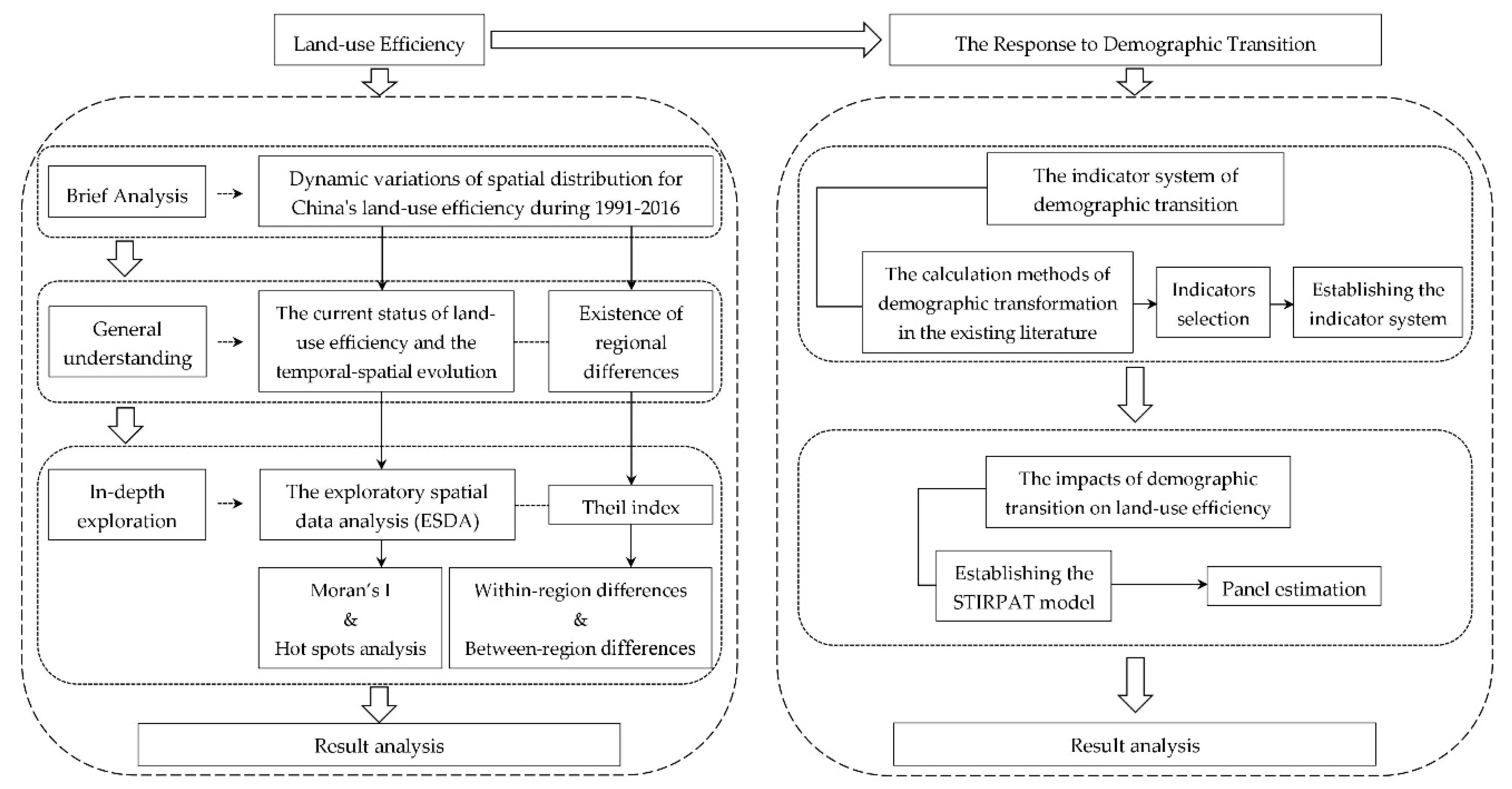
2. An Analytical Framework

Traditional studies on land-use efficiency mostly targeted one of the aspects only, such as the development status, temporal and spatial distribution, regional disparity, or influence factors of land-use efficiency; a few consider two or three aspects. Among them, they were either limited to one province or one region and were not extended to the whole country, or the research period was relatively short and only studied the land-use efficiency for several years [19,24,25,26,27]. In addition, among studies on the influence factors of land-use efficiency, there is still a lack of researches that focuses on the perspective of demographic transition. To sum up, this paper takes the land-use efficiency in China from 1991 to 2016 as the research object, and undertakes an intensive discussion on its current situation, temporal and spatial evolution characteristics, regional disparity, and the response to demographic transition. Figure 1 shows a specific analytical framework for the paper.

3. Methodology

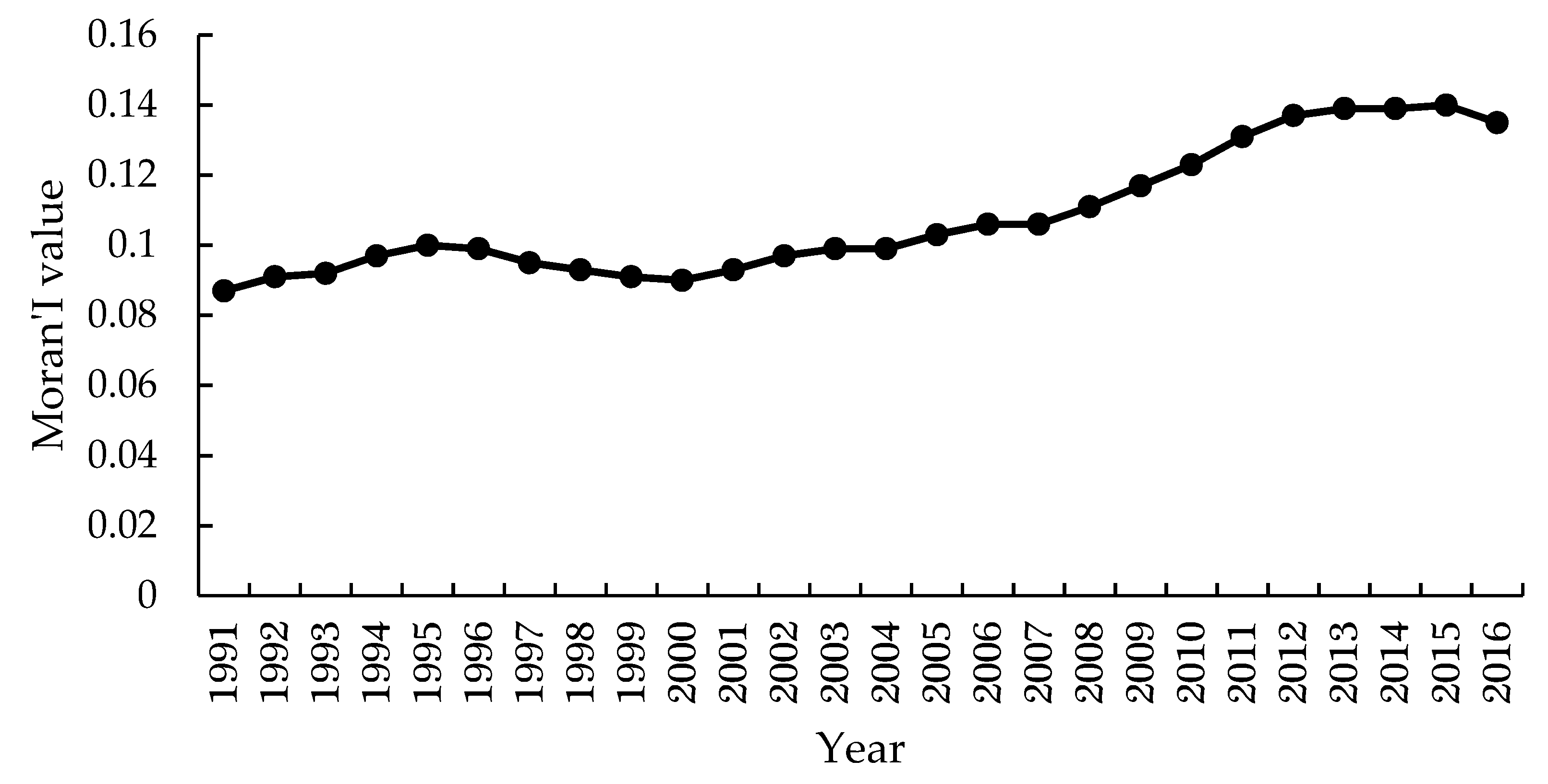
3.1. Exploratory Spatial Data Analysis (ESDA)

In order to study the land-use efficiency in China from the spatial perspective and uncover the spatial-temporal evolution and trend of land-use efficiency, exploratory spatial data analysis (ESDA) was used to study the spatial agglomeration model, evolution trend and hot spot distribution of the land-use efficiency. Since the 1990s, ESDA has developed rapidly [28]. The detection of ESDA was represented by global statistics and local statistics. In the existing literature related to spatial analysis, the commonly used global statistics are global Moran’s I and Getis’s C (Geary’s Contiguity Ratio); local statistics include local Moran’s I, Anselin’s LISA and Getis-Order G_i* [29,30,31,32]. Therefore, global Moran’s I and Getis-Order G_i* were selected to accomplish the exploration of the spatial agglomeration pattern in regard to land-use efficiency.

Global Moran’s I can be calculated from the following equation:

$$I=\frac{n{{\displaystyle \sum }}_{i=1}^n{{\displaystyle \sum }}_{j=1}^n{w}_{ij}\left(x_i-\overline{x}\right)\left(x_j-\overline{x}\right)}{{{\displaystyle \sum }}_{i=1}^n{{\displaystyle \sum }}_{j=1}^n{w}_{ij}{{\displaystyle \sum }}_{i=1}^n{\left(x_i-\overline{x}\right)}^2}, i\ne j$$

(1)

where n is the number of study spaces; x_i and x_j respectively represent the observed values of variable x on the spaces i and j; w is the spatial weight, which is the relationship between the spaces i and j, if two spaces are adjacent, w_ij = 1, or w_ij = 0; and $\overline{x}$ denotes the average of all observed values. Because Moran’s I statistics obey random distribution or approximate normal distribution, the significance test can be transformed into the calculation of Z-score, and the formula is as follows:

$$Z=\frac{I-E\left(I\right)}{\sqrt{VAR\left(I\right)}}$$

(2)

where E(I) denotes the expectation of Moran’s I; and VAR(I) is the variance of Moran’s I.

Global Moran’s I is the analysis of spatial distribution in the entire study space and will hide the local instability in a small range. However, using local spatial autocorrelation statistics can more accurately reveal the heterogeneity of spatial elements [33,34]. Therefore, we use Getis-Order G_i* to detect the heterogeneous characteristics of the spatial distribution of land-use efficiency. The formula is as follows:

$$G_i^{*}=\frac{{{\displaystyle \sum }}_{i=1}^n{{\displaystyle \sum }}_{j=1}^n{w}_{ij}{x}_j}{{{\displaystyle \sum }}_{j=1}^n{x}_j}, i\ne j$$

(3)

The meaning of each variable in Equation (3) is consistent with those of Equation (1).

To better reflect and explain the cluster degree or difference of extremely high or extremely low value elements in the whole study area, G_i* can be standardized by the following equation:

$$Z\left(G_i^{*}\right)=\frac{G_i^{*}-E\left(G_i^{*}\right)}{\sqrt{VAR\left(G_i^{*}\right)}}$$

(4)

where E(G_i*) means the expectation of G_i*; and VAR(G_i*) is the variance of G_i*.

3.2. Theil Index

Because the Theil index has additivity and decomposability, it has become an important method to measure inequality and difference [35], and it has been applied to many fields such as economic development inequality [36,37], household income inequality [38,39,40], regional energy consumption differences [41], CO₂ emission regional inequality [42,43,44] and so on. Thus, we employed the Theil index to measure the gaps in land-use efficiency among various regions and provinces in order to observe the changes in research gaps over time.

The Theil index T established in this study can be described by the following equation:

$$\mathrm{T}={\displaystyle \sum }_i{\displaystyle \sum }_j\left(\frac{Y_{ij}}{Y}\right)\log \left(\frac{Y_{ij}/Y}{S_{ij}/S}\right)$$

(5)

where Y_ij and S_ij denote the GDP and land area in province j of region i, respectively; so $Y={\displaystyle \sum }_i{\displaystyle \sum }_j{Y}_{ij}$ and $S={\displaystyle \sum }_i{\displaystyle \sum }_j{S}_{ij}$ are the total GDP and total land area of all provinces, respectively.

$$T_p={\displaystyle \sum }_j\frac{Y_{ij}}{Y_i}\log \left(\frac{Y_{ij}/Y_i}{S_{ij}/S_i}\right)$$

(6)

Equation (6) represents the gap in land-use efficiency among the provinces in region i. Hence, Equation (7) can be expressed as below:

$$\mathrm{T}={\displaystyle \sum }_i\left(\frac{Y_i}{Y}\right)T_p+{\displaystyle \sum }_i\left(\frac{Y_i}{Y}\right)\log \left(\frac{Y_i/Y}{S_i/S}\right)=T_{WG}+T_{BG}$$

(7)

where T_WG is the intraregional gaps, called the within-region differences; and T_BG denotes the regional gaps, called the between-region differences. They are shown as below:

$$T_{WG}={\displaystyle \sum }_i\left(\frac{Y_i}{Y}\right)T_p={\displaystyle \sum }_i{\displaystyle \sum }_j\left(\frac{Y_i}{Y}\right)\left(\frac{Y_{ij}}{Y_i}\right)\log \left(\frac{Y_{ij}/Y_i}{S_{ij}/S_i}\right)$$

(8)

$$T_{BG}={\displaystyle \sum }_i\left(\frac{Y_i}{Y}\right)\log \left(\frac{Y_i/Y}{S_i/S}\right)$$

(9)

In addition, $T_{WG}/T$ and $T_{BG}/T$ represent the contribution of within-group and between-region differences to the national gap, respectively.

3.3. The Indicator System of Demographic Transition

The researches on demographic transition in previous studies can be roughly divided into three aspects according to the focuses and research contents: transition of population size, transition of population structure and transition of population quality. For the transition of population size, scholars usually use the birth rate (including fertility rate), mortality rate, or population density as measurement indicators [45,46,47], and many scholars directly reflect the variation trend of demographic transition through the natural growth rate of the population [48,49].

For the transition of population structure, many studies are concerned with the changes of population age structure in different social environments, in which the population age is often expressed by the average life expectancy, expectation of life, the working-age population ratio, or the dependency ratio [45,50,51,52]. Meanwhile, with the development of urbanization in China, the transition of the urban–rural population structure has become a research hotspot for scholars, and is measured intuitively by the urbanization rate [53,54]. In addition, some scholars believe that the proportion of employment in the tertiary industry, and nonfarm payrolls ratio can also reflect the changes in urban–rural population structure to a certain extent [55,56].

In recent years, the transition of population quality has been the focus of discussions in academic circles, mainly from the perspective of the population education level and economic development degree as the starting point. The education level of the population is mostly measured by per capita years of education and the teacher-student ratio in primary education [57], while the degree of economic development is mainly determined by per capita GDP and per capita income [46].

Based on the actuality of demographic transition in China, combined with the research results from the numerous papers mentioned above, and considering the accessibility of the data, this paper selected some indicators which can represent China’s demographic transition, and constructed an indicator system of demographic transition (

Table 1. Indicator system of China’s demographic transition.

Synthetic Index	Type	Indicator (Variable)	Definition	Unit of Measurement
Demographic transition	Quantity transition	Population (P)	Total population at the end of the year	104 Person
	Structure transition	Working-age population ratio (WAP)	The ratio of people over 14 and under 65 years old in the total population	Percent
		Urbanization (URB)	The ratio of the urban population in the total population	Percent
		Nonfarm payrolls ratio (NFP)	The ratio of the nonfarm payrolls in the total working population	Percent
		Employment structure 2 (ES2)	Employment population of the secondary industry	104
		Employment structure 3 (ES3)	Employment population of the tertiary industry	104
	Quality transition	Per capita education (PEDU)	The average of the total number of years of education	Year
		Per capita GDP (PGDP)	GDP divided by the population at the end of the year	Yuan
		Land-use efficiency (LUE)	GDP divided by the area of land at the end of the year	108 Yuan/km2

). With this, we hoped to explore the driving factors of land-use efficiency in terms of population more systematically and comprehensively, and to provide a good scientific and theoretical basis for further improving the land-use efficiency.

3.4. STIRPAT Model

The STIRPAT model is often used to analyse the disproportionate impact of human factors on the environment. It is a research model that has been widely used in a large amount of literature, especially in papers on carbon emission and energy consumption [58,59,60,61], but its effect in land-use efficiency has not been well discussed. As we all know, land as a kind of natural resource that has a profound impact on the environment through its utilization mode and efficiency. Hence, in this paper, the STIRPAT model was used to study the influence of demographic transition on land-use efficiency. Initially, Ehrlich and Holdren [62] developed the IPAT model which was considered as a theoretical framework for analyzing the impacts of population, affluence and technological factors. The general IPAT model is demonstrated in the following equation:

$$I=P·A·T$$

(10)

where $I$ indicates the environmental impact; $P$is the population size; $A$denotes the level of affluence and economic development; and $T$is a technological factor. Dietz and Rosa [63] improved on the primary IPAT model and established the STIRPAT model. Subsequently, the STIRPAT model was further transformed by York et al. [64], and merged with other accessional factors, such as the nonfarm payrolls ratio and urbanization. Hence, the STIRPAT model combined social, economic and technical factors can be widely used to solve practical problems [65]. The general STIRPAT model can be expressed as below:

$$I_{it}=a{P}_{it}^b{A}_{it}^c{T}_{it}^d{e}_{it}$$

(11)

Then, Equation (11) takes the following form after taking logarithms:

$$\ln \left(I_{it}\right)=a+b\ln \left(P_{it}\right)+c\ln \left(A_{it}\right)+d\ln \left(T_{it}\right)+e_{it}$$

(12)

where $a$is a constant term; $P$, $A$ and $T$ are the same as in Equation (10); $b$, $c$ and $d$ are the coefficients of the impacts for $P$, $A$ and $T$, respectively; the suffixes $i$ and $t$ denote the region and time, respectively; and $e$ refers to the error term.

Some appropriate factors can be added to the STIRPAT model to evaluate their influences on the dependent variable. Therefore, to obtain a deeper understanding and comprehensively analyze the effects of China’s demographic transition on land-use efficiency, we expanded the STIRPAT model by introducing variables from the previously constructed demographic transition indicator system. Moreover, we introduced squared terms for population size, urbanization, the population employed in the secondary and tertiary industries, and per capita GDP to investigate whether there is a Kuznets relationship between these variables and land-use efficiency. The modified form of the complete STIRPAT model can be demonstrated as follows:

$$\begin{array}{ll}\ln \left(LU{E}_{it}\right)=& a_0+a_1\ln \left(P_{it}\right)+a_2{\left[\ln \left(P_{it}\right)\right]}^2+a_3\ln \left(WA{P}_{it}\right)+a_4\ln \left(UR{B}_{it}\right)+ a_5{\left[\ln \left(UR{B}_{it}\right)\right]}^2\\ & +a_6\ln \left(NF{P}_{it}\right)+a_7\ln \left(ES{2}_{it}\right)+a_8{\left[\ln \left(ES{2}_{it}\right)\right]}^2+ a_9\ln \left(ES{3}_{it}\right)+a_{10}{\left[\ln \left(ES{3}_{it}\right)\right]}^2\\ & + a_{11}\ln \left(PED{U}_{it}\right)+a_{12}\ln \left(PGD{P}_{it}\right)+a_{13}{\left[\ln \left(PGD{P}_{it}\right)\right]}^2+e_{it}\end{array}$$

(13)

4. Data Source

In order to ensure that our data was complete and available, a balanced panel dataset was collected. Our data was acquired from the China Statistical Yearbook (1991–2016) and the Statistical Yearbook of all provinces (1991–2016). The real GDP was measured based on constant prices. The working-age population was measured using the ratio of people over 14 and under 65 years old in all provinces. The urbanization rate was calculated by the ratio of the urban population to the total population. The nonfarm payrolls ratio was calculated according to the proportion of the nonfarm payrolls in the whole working population. Per capita education was measured based on the formula given by Yuan and Huang [48]. Land-use efficiency was calculated by dividing the area of land in each province by its GDP at the end of the year.

As the research aim of this paper includes exploring regional disparities in terms of the spatial distribution of land-use efficiency and its driving factors, we classified the 31 provinces of China into three regions: the eastern, central and western regions (

Table A1. Distribution of the 31 provinces in the three regions of China.

Regions	Provinces
Eastern	Liaoning, Shanghai, Jiangsu, Zhejiang, Tianjin, Fujian, Shandong, Hebei, Guangdong, Hainan, Beijing
Central	Shanxi, Jilin, Heilongjiang, Anhui, Jiangxi, Henan, Hubei, Hunan
Western	Sichuan, Chongqing, Guizhou, Yunnan, Shaanxi, Gansu, Ningxia, Inner Mongolia, Qinghai, Xizang, Xinjiang, Guangxi

in Appendix A).

5. Results

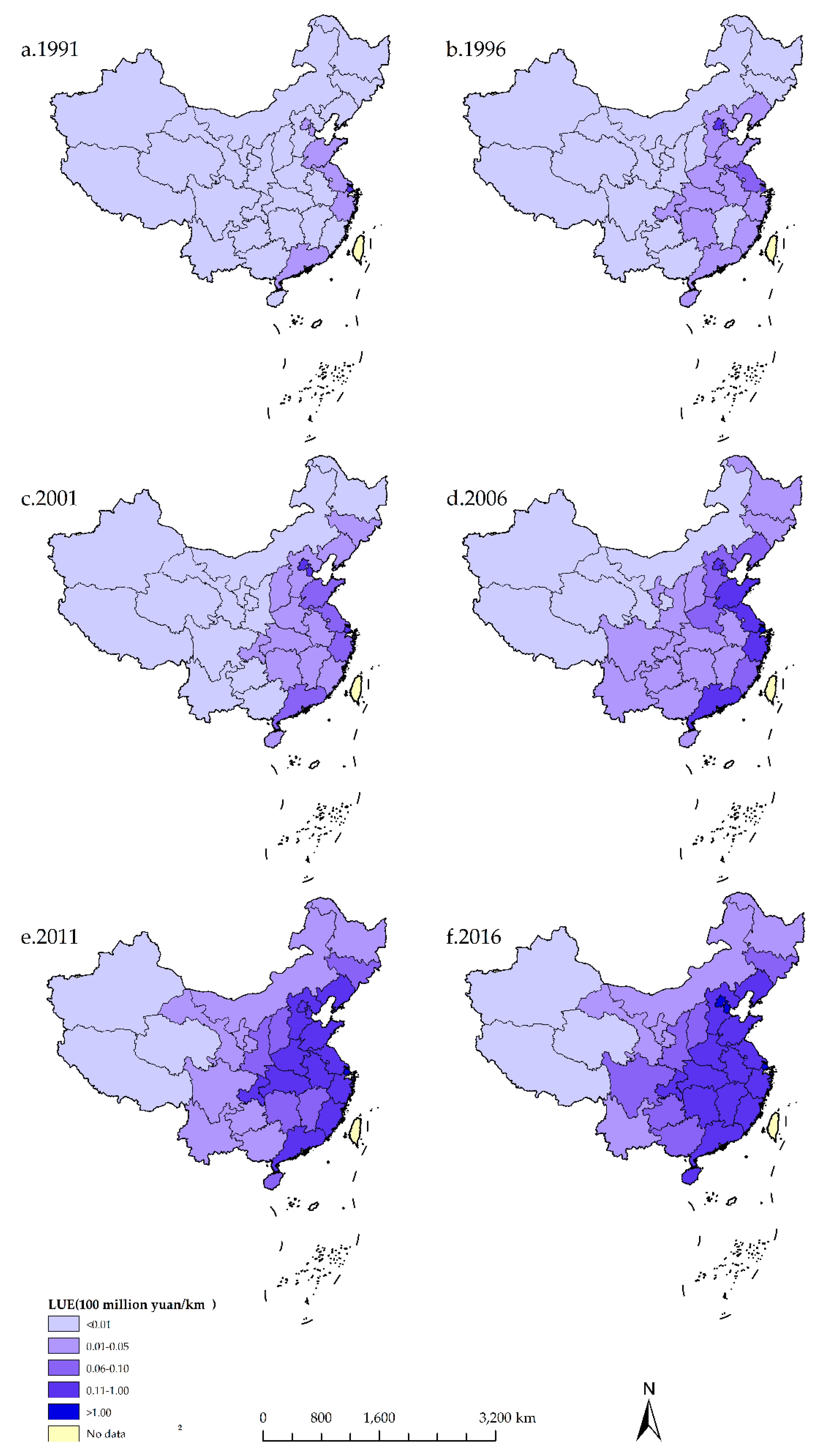
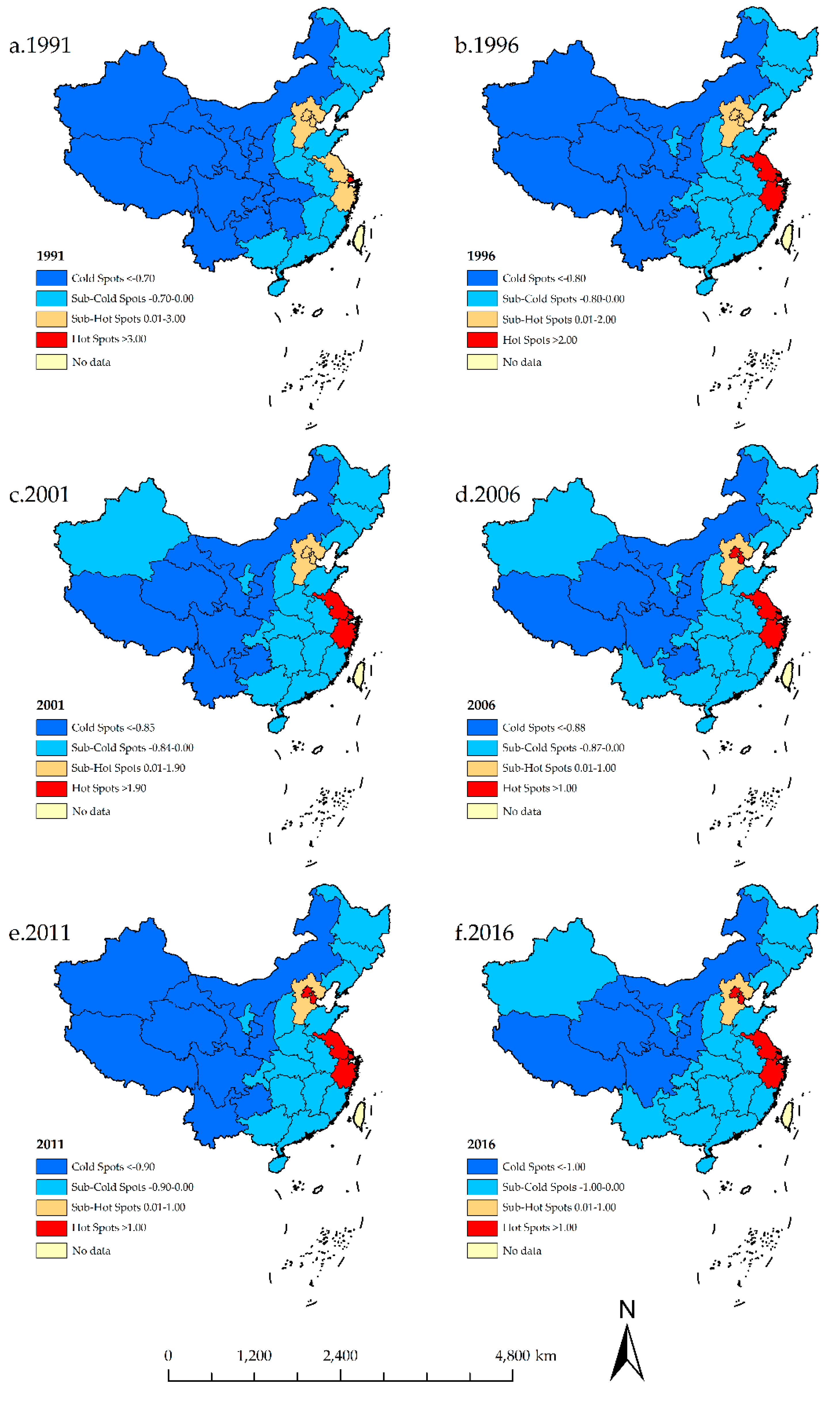
5.1. Dynamic Evolution of Spatial Distribution for Land-Use Efficiency

As shown in Figure 2, the spatial distribution of land-use efficiency in China has significant regional differences and spatial agglomeration characteristics from 1991 to 2016, which can be summarized into the following two points:

(1)

The land-use efficiency is the highest in the eastern region and the lowest in the western region, and gradually decreases from east to west. Shanghai’s land-use efficiency has been leading the country for 26 years.

(2)

The spatial agglomeration of land-use efficiency is mainly to take some provinces with dense population and developed economies in the eastern region into account as the cluster centers, such as Beijing, Shanghai, Tianjin, Zhejiang, Guangdong and so on. These provinces greatly promote the improvement of land utilization efficiency in their own and their surrounding provinces, forming a number of provincial clusters with higher land-use efficiency, which gradually spread over time. By 2016, the whole eastern and central regions had achieved very high or high land-use efficiency, and some western regions had also been affected, leading to improved land-use efficiency.

Figure A1 and

Table A2. Results and confidence intervals of global Moran’s I statistics.

Year	Moran’I	p-Value	Z-Score
1991	0.087	0.027	2.215
1992	0.091	0.02	2.321
1993	0.092	0.015	2.427
1994	0.097	0.013	2.492
1995	0.100	0.012	2.503
1996	0.099	0.013	2.482
1997	0.095	0.015	2.433
1998	0.093	0.017	2.384
1999	0.091	0.019	2.34
2000	0.090	0.022	2.294
2001	0.093	0.023	2.267
2002	0.097	0.023	2.268
2003	0.099	0.022	2.298
2004	0.099	0.022	2.296
2005	0.103	0.019	2.343
2006	0.106	0.018	2.374
2007	0.106	0.017	2.379
2008	0.111	0.016	2.401
2009	0.117	0.018	2.372
2010	0.123	0.016	2.417
2011	0.131	0.015	2.445
2012	0.137	0.015	2.443
2013	0.139	0.015	2.44
2014	0.139	0.015	2.428
2015	0.140	0.015	2.428
2016	0.135	0.016	2.412

show that all of the global Moran’s I statistics are positive, and Z(I) > 1.96, p < 0.05, indicating the land-use efficiency of China from 1991 to 2016 has positive spatial autocorrelation at the significance level of 0.05 and shows convergence. At the same time, the value of Moran’s I showed an overall upward trend, from 0.087 in 1991 to 0.135 in 2016. This indicates the spatial distribution of land-use efficiency is not random, presenting a significant spatial aggregation effect in the adjacent provinces, and this agglomeration characteristic was significantly enhanced.

Using the Hot Analysis tool of ArcGIS 10.2, the provincial administrative region was used as the evaluation unit to carry out the cold and hot spots analysis of land-use efficiency in China from 1991 to 2016. The results show that the spatial clustering differentiation degree of the land-use efficiency differs greatly in China (Figure 3). The values of Z(G_i*) are divided from low to high into four differentiation types, called Cold Spots, Sub-Cold Spots, Sub-Hot Spots, and Hot Spots, in turn. These four differentiation types reflect the spatial agglomeration degree of land-use efficiency in different regions. From the spatial perspective, the spatial distribution of cold and hot spot presents significant regional differences. Hot spots and sub-hot spots are mainly distributed in the Jiangsu-Zhejiang-Shanghai Region as well as the Beijing-Tianjin-Hebei Region. The cold spots are concentrated in the western region, and the sub-cold spots are concentrated in the central region. From the perspective of temporal evolution, regions with hot spots distribution have gradually grown from 1 in 1991 to 5 in 2016. Except for Shanghai, which has remained a hot spot, the others have been transformed from provinces where sub-hot spots were located in 1991. The provinces with cold spots distributions gradually reduced from 13 in 1991 to 6 in 2016, and the reduced 7 provinces were gradually turned into the sub-cold spot distribution regions, which increased the number of provinces with sub-cold spots distributions from 12 in 1991 to 19 in 2016.

5.2. Regional Disparities of Land-Use Efficiency

It can be seen from the spatial analysis that, significant regional difference of spatial distribution exists in the field of land-use efficiency in China, such that the development and changes of regional differences during the period of 1991–2016 needs to be studied further. The analysis and calculation of the Theil index was carried out under this context.

Table 2. Calculation results of Theil index.

Year	Theil Index						Contribution (%)
	Overall	Between-Region Differences	Within-Region Differences	Within-Region Differences in Three Regions			Between-Region Differences	Within-Region Differences	Within-Region Differences in Three Regions
				Eastern Region	Central Region	Western Region			Eastern Region	Central Region	Western Region
1991	0.41901	0.29345	0.15535	0.05409	0.00997	0.09128	70.03	37.07	12.91	2.38	21.79
1992	0.42910	0.30429	0.15365	0.05453	0.01028	0.08883	70.91	35.81	12.71	2.40	20.70
1993	0.44112	0.31787	0.15108	0.05378	0.01032	0.08697	72.06	34.25	12.19	2.34	19.72
1994	0.44488	0.32183	0.15060	0.05308	0.01023	0.08730	72.34	33.85	11.93	2.30	19.62
1995	0.45224	0.32499	0.15428	0.05580	0.01180	0.08668	71.86	34.12	12.34	2.61	19.17
1996	0.44982	0.32205	0.15492	0.05508	0.01213	0.08771	71.60	34.44	12.24	2.70	19.50
1997	0.45226	0.32363	0.15565	0.05666	0.01202	0.08697	71.56	34.42	12.53	2.66	19.23
1998	0.45399	0.32412	0.15697	0.05792	0.01222	0.08682	71.39	34.58	12.76	2.69	19.12
1999	0.45796	0.32729	0.15763	0.05989	0.01216	0.08558	71.47	34.42	13.08	2.66	18.69
2000	0.47808	0.34524	0.15835	0.06788	0.01190	0.07857	72.22	33.12	14.20	2.49	16.44
2001	0.47047	0.33494	0.16174	0.06709	0.01294	0.08171	71.19	34.38	14.26	2.75	17.37
2002	0.48508	0.34911	0.16112	0.07180	0.01223	0.07709	71.97	33.22	14.80	2.52	15.89
2003	0.48882	0.35317	0.16057	0.07320	0.01212	0.07526	72.25	32.85	14.97	2.48	15.40
2004	0.49137	0.35272	0.16353	0.07569	0.01311	0.07473	71.78	33.28	15.40	2.67	15.21
2005	0.49384	0.35762	0.16089	0.07492	0.01306	0.07291	72.42	32.58	15.17	2.65	14.76
2006	0.49445	0.35852	0.16071	0.07500	0.01325	0.07246	72.51	32.50	15.17	2.68	14.65
2007	0.49337	0.35584	0.16254	0.07521	0.01399	0.07333	72.12	32.94	15.24	2.84	14.86
2008	0.47417	0.33905	0.16163	0.06843	0.01438	0.07883	71.51	34.09	14.43	3.03	16.62
2009	0.47244	0.33629	0.16298	0.06711	0.01504	0.08083	71.18	34.50	14.20	3.18	17.11
2010	0.46557	0.33190	0.16072	0.06459	0.01491	0.08122	71.29	34.52	13.87	3.20	17.45
2011	0.45204	0.31972	0.16049	0.06042	0.01471	0.08535	70.73	35.50	13.37	3.25	18.88
2012	0.44459	0.31202	0.16154	0.05837	0.01506	0.08811	70.18	36.33	13.13	3.39	19.82
2013	0.44356	0.30932	0.16360	0.05850	0.01555	0.08955	69.73	36.88	13.19	3.51	20.19
2014	0.44422	0.30731	0.16651	0.05921	0.01644	0.09086	69.18	37.48	13.33	3.70	20.45
2015	0.45033	0.30907	0.17072	0.06111	0.01747	0.09213	68.63	37.91	13.57	3.88	20.46
2016	0.45948	0.30827	0.18071	0.06751	0.01884	0.09436	67.09	39.33	14.69	4.10	20.54

shows the calculation results of the Theil index of 31 Chinese provinces during the period of 1991–2016. Obviously, the change of the Theil index is small, and is actually in an ever-rising tendency in general: it increased from 0.41901 in 1991 to 0.45948 in 2016, growing by 8.81%. This shows that the inequality of land-use efficiency in various provinces has been increasingly enlarged.

The Theil index can be decomposed into two parts: within-region differences and between-region differences. The results for these parts are also shown in the Table 2. During 1991–2016, the between-region differences increased by 4.81% while the within-region differences significantly increased from 0.15535 in 1991 to 0.18071 in 2016, which shows a 14.04% increase, larger than that of both the overall and between-region differences. To sum up, the Theil index increase of the research period is the results of the simultaneous rise in within-region differences and between-region differences.

In order to explain the impact of different regions on the overall differences more clearly, the contribution of within-region differences and between-region differences to the Theil index can also be analyzed. As shown in Table 2, the contribution of within-region differences increased from 37.07% in 1991 to 39.33% in 2016, and the contribution of between-region differences decreased from 70.03% to 67.09%, while the average contribution of within-region differences and between-region differences were 34.78% and 71.12%, respectively. Hence, although the contribution of between-region differences to the regional difference tended to decline, it was still the decisive factor affecting the overall disparities. Further, since the launching of the Western Development Strategy in 2006, the within-region differences contribution rate of the western region group has maintained an increasing tendency, showing a rise from 14.65% in 2006 to 20.54% in 2016. Nevertheless, the within-region differences in the eastern and central regions have not changed significantly, remaining at around 12%–15% and 2%–4%, respectively.

5.3. Response of Land-Use Efficiency to Demographic Transition

In this paper, we estimate the panel data of 31 provinces in China from 1991 to 2016 with the STIRPAT model to explore the impact of population transformation on land-use efficiency. First, we use three panel unit root tests to ensure that the variables were effective and stable, namely the Im–Pesaran–Shin (IPS) test, the Fisher Augmented Dicky–Fuller (ADF) test, and the Fisher Phillips–Perron (PP) test. The results (

Table A3. Results of panel unit root tests at the nationwide level.

Unit Root Test	Variable	IPS	Fisher ADF	Fisher PP
Levels	lnP	−2.835 ***	124.895 ***	221.878 ***
	lnWAP	0.078	48.712	38.344
	lnURB	−1.241	69.920	61.693
	lnNFP	1.102	63.538	90.799 **
	lnES2	1.900	42.542	34.908
	lnES3	2.787	94.345 ***	152.944 ***
	lnPEDU	1.692	33.251	40.340
	lnPGDP	−0.991	90.600 **	113.533 ***
	lnLUE	0.801	54.866	97.816 ***
First difference	lnP	−23.536 ***	518.501 ***	537.371 ***
	lnWAP	−22.161 ***	493.191 ***	575.572 ***
	lnURB	−16.058 ***	341.800 ***	359.686 ***
	lnNFP	−12.375 ***	266.586 ***	279.100 ***
	lnES2	−11.949 ***	258.703 ***	277.294 ***
	lnES3	−18.570 ***	408.794 ***	424.017 ***
	lnPEDU	−30.828 ***	687.972 ***	811.876 ***
	lnPGDP	−6.317 ***	146.169 ***	112.627 ***
	lnLUE	−5.353 ***	135.480 ***	89.779 **

Note: The symbols *, ** and *** denote that p < 0.10, p < 0.05 and p < 0.01, respectively.

,

Table A4. Results of the panel unit root tests in the eastern region.

Unit Root Test	Variable	IPS	Fisher ADF	Fisher PP
Levels	lnP	1.998	16.993	36.890 **
	lnWAP	0.900	11.205	12.105
	lnURB	−1.604 *	29.160	25.741
	lnNFP	0.240	17.218	23.109
	lnES2	1.879	7.680	6.717
	lnES3	1.691	24.820	66.844 ***
	lnPEDU	0.005	17.713	22.281
	lnPGDP	−3.136 ***	65.025 ***	86.239 ***
	lnLUE	−0.910	32.036 *	67.598 ***
First difference	lnP	−16.401 ***	211.872 ***	216.456 ***
	lnWAP	−11.017 ***	146.206 ***	166.406 ***
	lnURB	−8.693 ***	109.274 ***	111.074 ***
	lnNFP	−5.453 ***	67.717 ***	61.697 ***
	lnES2	−5.749 ***	72.908 ***	74.946 ***
	lnES3	−10.639 ***	140.855 ***	119.799 ***
	lnPEDU	−17.319 ***	230.945 ***	267.447 ***
	lnPGDP	−3.904 ***	48.723 ***	45.641 ***
	lnLUE	−3.416 ***	48.808 ***	44.350 ***

Note: The symbols *, ** and *** denote that p < 0.10, p < 0.05 and p < 0.01, respectively.

,

Table A5. Results of the panel unit root tests in the central region.

Unit Root Test	Variable	IPS	Fisher ADF	Fisher PP
Levels	lnP	−2.803 ***	34.434 ***	45.985 ***
	lnWAP	−1.313	21.368	10.376
	lnURB	−0.286	13.055	13.675
	lnNFP	1.738	8.107	23.231
	lnES2	−0.220	17.301	15.030
	lnES3	0.285	32.389 ***	31.888 **
	lnPEDU	0.978	7.755	12.099
	lnPGDP	−0.077	13.057	14.865
	lnLUE	0.921	9.402	16.556
First difference	lnP	−12.505 ***	139.295 ***	139.468 ***
	lnWAP	−11.166 ***	126.031 ***	160.043 ***
	lnURB	−7.531 ***	80.748 ***	80.836 ***
	lnNFP	−4.725 ***	51.479 ***	59.174 ***
	lnES2	−5.065 ***	53.559 ***	52.214 ***
	lnES3	−8.239 ***	93.263 ***	102.663 ***
	lnPEDP	−14.729 ***	167.376 ***	207.988 ***
	lnPGDP	−4.213 ***	46.903 ***	46.738 ***
	lnLUE	−5.167 ***	57.552 ***	41.854 ***

Note: The symbols *, ** and *** denote that p < 0.10, p < 0.05 and p < 0.01, respectively.

and

Table A6. Results of the panel unit root tests in the western region.

Unit Root Test	Variable	IPS	Fisher ADF	Fisher PP
Levels	lnP	−4.200 ***	73.468 ***	139.004 ***
	lnWAP	0.345	16.139	15.863
	lnURB	−0.225	27.706	22.277
	lnNFP	0.144	38.213 **	44.459 ***
	lnES2	1.425	17.562	13.161
	lnES3	2.625	37.136 **	54.213 ***
	lnPEDU	1.987	7.782	5.960
	lnPGDP	1.628	12.519	12.430
	lnLUE	1.463	13.428	13.662
First difference	lnP	−11.934 ***	167.335 ***	181.448 ***
	lnWAP	−15.988 ***	220.954 ***	249.123 ***
	lnURB	−11.337 ***	151.778 ***	167.777 ***
	lnNFP	−10.840 ***	147.390 ***	158.229 ***
	lnES2	−9.580 ***	132.236 ***	150.135 ***
	lnES3	−12.928 ***	174.675 ***	201.555 ***
	lnPEDP	−20.973 ***	289.652 ***	336.441 ***
	lnPGDP	−4.651 ***	62.194 ***	56.576 ***
	lnLUE	−3.658 ***	54.204 ***	42.189 **

Note: The symbols *, ** and *** denote that p < 0.10, p < 0.05 and p < 0.01, respectively.

) show that many variables are nonstationary sequences. Nevertheless, when we looked at first-order difference for all data, every sequence was steady. Thus, the relationship between all variables could be further examined using the co-integration test. We carried out the co-integration test by Kao [66]. As is shown in

Table A7. Results of Kao panel cointegration test.

Cointegration Test	All Provinces	Eastern Region	Central Region	Western Region
ADF stat	−13.723 ***	−9.075 ***	−9.922 ***	−12.921 ***
Residual variance	0.000303	0.000223	0.000133	0.000450
HAC variance	0.000157	0.000156	0.0000869	0.000172

Note: The symbols *, ** and *** denote that p < 0.10, p < 0.05 and p < 0.01, respectively.

, we proved a long-term co-integrated relationship exists among all the variables for the nationwide level and for the three regions during the period of our study. Next, robust Hausman and likelihood ratio tests were employed to determine which panel estimation model should be selected. The results indicated that these two tests rejected the null hypothesis, and the FE model was selected (

Table A8. Panel data model selection.

	All Province	Eastern Region	Central Region	Western Region
Hausman test	63.772 ***	51.713 ***	12.459 ***	43.452 ***
Likelihood ratio test	64.827 ***	50.667 ***	67.674 ***	43.375 ***
Model type	FE	FE	FE	FE

Note: The symbols *, ** and *** denote that p < 0.10, p < 0.05 and p < 0.01, respectively.

). In addition, we explored the autocorrelation by employing the Wooldridge test [67]. The Wald test [68] was adopted to inspect groupwise heteroscedasticity. For the nationwide sample, we employed the CD test [69] to explore cross-sectional dependence. In the three regions, the Breusch–Pagan LM test [68] was used to examine the cross-sectional dependence of all sequences. Based on these tests, we confirmed that groupwise heteroscedasticity and cross-sectional dependence existed in all datasets. However, with the exception of the eastern region, we found that autocorrelation did not exist. Because of the test results above, our regression estimation used four regression approaches, FE, FGLS, PCSE and DK.

5.3.1. The Analysis of Response in the Whole Country

Table 3. Estimation results for the land-use efficiency models.

Variable	The Whole Sample				Eastern Region
	FE(1)	FGLS(2)	PCSE(3)	DK(4)	FE(5)	FGLS(6)	PCSE(7)	DK(8)
lnP	1.574 ***	1.901 ***	1.963 ***	1.574 **	1.516 ***	1.708 ***	1.839 ***	1.516 **
(lnP) *	−0.0849 ***	−0.0993 ***	−0.102 ***	−0.0849 **	−0.0804 ***	−0.0856 ***	−0.0934 ***	−0.0804 *
lnWAP	−0.00712	−0.0210 ***	−0.0272	−0.00712	0.0630	0.0155	0.0270	0.0630
lnURB	0.00435	0.00369 ***	0.00640	0.00435	0.00409	0.00184	0.00948	0.00409
(lnURB) *	−0.000166	0.000289	0.00162	−0.000166	0.00593	0.00421	0.00919	0.00593
lnNFP	−0.00892	−0.0251 ***	−0.0374	−0.00892	0.0549	0.000719	−0.0480	0.0549
lnES2	−0.0221	−0.0381 ***	−0.050 3 **	−0.0221	0.0161	−0.153 **	−0.119	0.0161
(lnES2) *	0.00502	0.00612 ***	0.00764 ***	0.00502	0.00205	0.0131 ***	0.0124	0.00205
lnES3	0.126 *	0.0756 ***	0.0845	0.126	−0.114	0.105	0.110	−0.114
(lnES3) *	−0.00973	−0.00468 ***	−0.00498	−0.00973	0.00958	−0.00716	−0.00639	0.00958
lnPEDU	0.0121	0.0181 ***	0.0149	0.0121	0.0546 *	0.0380 ***	0.0649 *	0.0546 *
lnPGDP	1.147 ***	1.072 ***	1.070 ***	1.147 ***	1.096 ***	1.069 ***	1.042 ***	1.096 ***
(lnPGDP) *	−0.0121 ***	−0.00797 ***	−0.00765 *	−0.0121 *	−0.00771 **	−0.00508 ***	−0.00417	−0.00771
Constant	0.0156 ***	0.0143 ***	0.0136 ***	0.0156 **	0.0137 ***	0.00929 ***	0.0108 ***	0.0137 **
R*	0.947		0.943		0.971		0.966
Autocorrelation test	F(1,30) = 0.006				F(1,10) = 5.492 **
Cross-sectional dependence test	16.256 ***				209.157 ***
dependence test
Heteroscedasticity test	χ * (31) = 10136.37 ***				χ * (11) = 434.25 ***
Observations	775	775	775	775	275	275	275	275
Variable	Central Region				Western Region
	FE(9)	FGLS(10)	PCSE(11)	DK(12)	FE(13)	FGLS(14)	PCSE(15)	DK(16)
lnP	3.187	4.120 ***	4.235 ***	3.187 *	0.463	0.844 ***	0.729	0.463
(lnP) *	−0.181	−0.235 ***	−0.242 ***	−0.181 *	−0.0203	−0.0376 ***	−0.0338	−0.0203
lnWAP	−0.0343	−0.0380	−0.0299	−0.0343	−0.0352	−0.0169	−0.0374	−0.0352
lnURB	0.0225	0.0261 ***	0.0228 *	0.0225	0.00775	0.0101	0.00851	0.00775
(lnURB) *	0.00340	0.00636	0.00338	0.00340	0.00126	0.00345	0.00201	0.00126
lnNFP	−0.0350	−0.0254	−0.0212	−0.0350	0.00356	−0.0180	−0.0129	0.00356
lnES2	−0.291	−0.131	−0.194	−0.291	−0.00363	0.0166	−0.00899	−0.00363
(lnES2) *	0.0275	0.0121 *	0.0191	0.0275	0.00307	−0.000383	0.00353	0.00307
lnES3	0.113	0.134	0.237	0.113	0.231 *	0.131 ***	0.230 ***	0.231
(lnES3) *	−0.00992	−0.0100	−0.0201	−0.00992	−0.0204 *	−0.0107 ***	−0.0193 ***	−0.0204
lnPEDU	0.0307	0.0203	0.0329	0.0307	−0.00323	0.000613	−0.00417	−0.00323
lnPGDP	1.162 ***	1.156 ***	1.144 ***	1.162 ***	1.160 ***	1.095 ***	1.128 ***	1.160 ***
(lnPGDP) *	−0.0114 ***	−0.00976 ***	−0.0104***	−0.0114 **	−0.0159 ***	−0.00863 ***	−0.0140*	−0.0159 *
Constant	0.00930 ***	0.00545 ***	0.00965 ***	0.00930 **	0.0225 ***	0.0130 ***	0.0216 ***	0.0225 *
R*	0.975		0.975		0.905		0.904
Autocorrelation test	F(1,7) = 0.295				F(1,11) = 0.001
Cross-sectional dependence test	52.163 ***				385.329 ***
dependence test
Heteroscedasticity test	χ * (8) = 348.91 ***				χ * (12) = 2700.80 ***
Observations	200	200	200	200	300	300	300	300

Note: The symbols *, ** and *** denote that p < 0.10, p < 0.05 and p < 0.01, respectively.

shows the results of the panel estimation. Model 4 is relevant for the national level. The effects of lnP and its squared term on land-use efficiency, which reflect the transformation of the population size, are both significant at the 5% level. It is worthwhile to note that the coefficient of lnP is 1.574, and the squared term of lnP is −0.0849, so we identified an inverted U-curve relationship between land-use efficiency and population growth. Land-use efficiency first increases up to the population threshold of 10,611.877 × 10⁴, then efficiency decreases as the population grows. The overall average population in the whole country is 4117.753 × 10⁴, which is smaller than the identified threshold. Per capita GDP has significant influence on land-use efficiency at the 1% level, and it increases land-use efficiency with an elasticity of 1.147. The squared term of lnPGDP is also statistically significant and decreases land-use efficiency with an elasticity of −0.0121. Thus, we confirmed a Kuznets curve relationship between land-use efficiency and per capita GDP.

For the three regions, the cross-sectional dimensions are smaller than the time dimensions. Thus, we focused on models 6, 10 and 14.

5.3.2. The Analysis of Response in the Eastern Region

For the eastern region, the cross-sectional dimensions are smaller than the time dimensions. Thus, we focused on model 6. The result shows that the elasticities of lnP and its squared term are 1.708 and −0.0856, respectively, and they were all significant at the 1% level. Hence, we demonstrated there is an inverted U-curve relationship between land-use efficiency and population in the eastern region. In particular, land-use efficiency increases up to the population threshold of 21,517.794 × 10⁴, while the overall average level of the population in the eastern region is 4568.902 × 10⁴, which means that it is smaller than the identified threshold. Therefore, land-use efficiency will increase up to the threshold for the development of population size, then decrease as the population increases. The first term of lnES2 is significant at the 5% level. Furthermore, the elasticity for the first term of lnES2 is −0.153, and the coefficient of the squared term is 0.0131, which proves a U-shaped curve relationship between the population employed in secondary industries and land-use efficiency in the eastern region. Land-use efficiency decreases down to the ES2 threshold of 343.674 × 10⁴ for the eastern region, whereas the overall average ES2 is 874.976 × 10⁴, indicating that this region has reached the turning point where land-use efficiency will improve as the population employed in secondary industries increases. Per capita education increases land-use efficiency with an elasticity of 0.0380, which has a significantly positive effect on the dependent variable at the 1% level. The coefficients for lnPGDP and its squared term are 1.069 and −0.00508, respectively, and they have significant influences at the 1% level. Hence, we confirmed a Kuznets curve relationship between land-use efficiency and per capita GDP in the eastern region.

5.3.3. The Analysis of Response in the Central Region

For the central region, we focused on model 10. The result shows that the coefficient of lnP is the largest (4.120) and significant at the 1% level, which suggests that population size is a major factor for land-use efficiency. However, the elasticity of the squared term has a significantly negative (−0.235) influence on the dependent variable. That means there is an inverted U-curve relationship between land-use efficiency and population size. Land-use efficiency increases up to the population threshold of 6412.198 × 10⁴, but the overall average population size in the central region is 5217.413 × 10⁴. Thus, for central region provinces, land-use efficiency will increase nonmonotonically with an increasing population. The first and squared terms of urbanization are both positive (0.0261 and 0.00636, respectively), so we cannot identify a Kuznets curve relationship between land-use efficiency and the degree of urbanization. The elasticities of per capita GDP and its squared term are 1.156 and −0.00976, respectively, and they are statistically significant. That indicates an inverted U-curve relationship between land-use efficiency and per capita GDP. The squared term of lnES2 increases land-use efficiency with a coefficient of 0.0121.

5.3.4. The Analysis of Response in the Western Region

For the western region, the cross-sectional dimensions are smaller than the time dimensions. Thus, we focused on model 14. The result shows that the elasticities of population size and its squared term are 0.844 and −0.0376, and they have significant influences on land-use efficiency at the 1% level. Hence, we identified that an inverted U-curve relationship exists between land-use efficiency and population growth. Furthermore, land-use efficiency increases up to the population threshold of 74,862.191 × 10⁴. The overall average population of the western region is 2971.093 × 10⁴, which is smaller than the identified threshold. The first term for ES3 has a significant and positive (0.131) impact at the 1% level, while the squared term is statistically significant but negative (−0.0107). Thus, we confirmed a Kuznets curve relationship between the population employed in tertiary industries and land-use efficiency in the western region. Land-use efficiency increases up to the ES3 threshold of 455.545 × 10⁴, and then decreases with an increasing population employed in tertiary industries, whereas the overall average ES3 in the western region is 415.97 × 10⁴, which is smaller than the identified threshold. The first and squared terms of per capita GDP have significant influences on land-use efficiency at the 1% level, with elasticities of 1.095 and −0.00863. Therefore, we confirmed a Kuznets curve relationship between land-use efficiency and per capita GDP in the western region.

6. Discussion

6.1. Temporal-Spatial Distribution Characteristics and Regional Disparities of Land-Use Efficiency

Based on the above explanation of spatial analysis results, the spatial distribution of land-use efficiency in China has a significant agglomeration effect and regional disparities. During 1991–2016, although China’s overall land-use efficiency increased significantly, the spatial pattern of the overall distribution has not changed significantly, and its characteristics are mainly reflected in two aspects. First, the more developed the regions are in socio-economic and other aspects, the better the land-use efficiency. Second, the average level of land-use efficiency presents a huge east-west disparity. This is mainly because the eastern region has more prominent superiorities over other regions in terms of geographical location, transportation and resources, and so on, which has enabled this region to attract a large amount of capital investment in the wake of the reform and opening up, thus greatly promoting the land-use efficiency and leading to this region becoming the hot spot concentration area of land-use efficiency.

6.2. Response of Land-Use Efficiency to Demographic Quantity Transition

For all indicators, the quantity transition of population is statistically significant for the whole country and the three regions. Population size is a comprehensive reflection of the economic development level, the environmental capacity, and the land-use status, and it has a strong explanatory power regarding land-use efficiency for the nationwide level and for the three regions. Population size is the main demographic factor affecting land-use efficiency, which is consistent with the conclusions of most existing research. Furthermore, a Kuznets curve relationship exists between land-use efficiency and population in all samples. The reason is that land-use tends to be relatively extensive in the initial stage of population growth. As the population size expands, land-use will develop in an intensive direction. Thus, the land-use efficiency improves. However, when the population increases beyond a certain threshold, there may be problems of congestion and inefficiency in functional areas. These problems indicate a decrease in land-use efficiency, as represented by the decline of the older urban areas. At present, the land-use efficiency at the national level and in the three individual regions is continuing to experience an upward trend as the population becomes more concentrated in urban areas. This is because the government has implemented many urban planning and construction projects, greatly improving the functions and efficiency of the land.

6.3. Response of Land-Use Efficiency to Demographic Structure Transition

In the indicators reflecting the demographic structure transition, the results showed that the urbanization degree has strong explanatory power in relation to land-use efficiency in the central region. Furthermore, China is now in a period where land-use efficiency will improve as the urbanization rate increases. On the one hand, cities are constantly expanding outward in the process of urbanization, and the demand for construction land is increasing correspondingly. However, because total land resources are limited, land-use has evolved spontaneously from the original scattered distribution pattern to a clustering pattern. This has gradually improved land-use efficiency and alleviated the increasingly acute contradictions between supply and demand of urban construction land. On the other hand, the development of urbanization will directly promote economic development [70], which means that an increase in land-use inputs and the optimization of this input structure will facilitate the promotion of land-use efficiency [71].

The population employed in secondary industries and per capita education have significant influences on land-use efficiency in the eastern region. What is more, the empirical results confirmed a U-shaped curve relationship between the population employed in secondary industries and land-use efficiency. This is because the secondary industries of the eastern region took the lead in the process of national economic development. In the early years, the rapid expansion and extensive management of the secondary industries reduced land-use efficiency. However, following improvements in the level of land marketization and a rise of land prices, the industrial sector has gradually adopted scale management [72], which has enhanced land-use efficiency. At the same time, a Kuznets curve relationship exists between the population employed in tertiary industries and land-use efficiency in the western region, and the former could improve the latter at the current stage of development. The existing literature reveals that promoting the flow of labor factor inputs to tertiary industry is the major means for improving the land-use efficiency [73]. This is because, compared with primary and secondary industries, tertiary industry has the advantage of requiring less land and yielding higher profits. As the tertiary industry is growing and developing in the western region, high-quality laborers are shifting to the new service industries, especially the upmarket service industries. The establishment and perfection of the urban modern service system and the optimization and upgrading of the industrial structure not only optimizes the allocation of labor, it also raises the land-use efficiency. Nevertheless, when the population employed in tertiary industries has risen to a certain point, excessive inputs by tertiary industry practitioners will reduce the efficiency of land inputs and outputs in this industry. Redundancy will also occur in the investment in assets and construction land by tertiary industry [74], leading to a decline in the land-use efficiency.

6.4. Response of Land-Use Efficiency to Demographic Quality Transition

The improvement of human capital level, which represents the demographic quality transition, plays an important role in advancing land-use efficiency in the eastern region. Compared with the other two regions, the eastern region has the strongest human capital levels. Beijing, Shanghai, Guangdong, Jiangsu and other eastern regional provinces possess the highest comprehensive human capital scores in the whole country [75]. This means that there are greater challenges involved in the allocation of human resources, but this process will boost the improvement of land-use efficiency.

Per capita GDP is an important indicator that represents residential affluence and transitions in income levels. We proved that it has a significant influence on the dependent variable in the nationwide sample, and for the three regions. Further, land-use efficiency will improve nonmonotonically as per capita GDP increases. With increases in economic growth and people’s living standards, tertiary industries have continued to increase their demands for land. The contribution of tertiary industries to increases in GDP has been rising on a yearly basis; in 2016, tertiary industries accounted for to 58.2% of GDP growth, up from 39% in 2010. In line with this, land-use by tertiary industry increased gradually, enhancing land-use efficiency. However, these impacts will reach a threshold value after the economy reaches a certain development point. Thus, other factors are required to enhance land-use efficiency in the future.

7. Conclusions and Implications

According to the exploration of the spatial distribution pattern of land-use efficiency in China from 1991 to 2016, we found land-use efficiency has a significant and positive spatial autocorrelation, indicating that there exists a spatial agglomeration effect, and most of the cluster centers are areas with a dense population and developed economy. Meanwhile, we undertook a furtherer study on the inequal distribution of land-use efficiency reflected by spatial analysis. The results suggested that the regional differences in land-use efficiency have a gradual upward trend in general, and between-region differences are the decisive factor affecting the overall regional disparity.

We took China’s demographic transition as the entry point to analyze the driving forces of land-use efficiency. In the whole country, transition of population size and transition of income levels are double-edged swords for land-use efficiency. When they grow too high, land-use efficiency will decline, and transition of population size and transition of income levels are also the primary cause for regional differences in the spatial distribution of land-use efficiency. Further research has shown that the impacts of demographic transition on land-use efficiency varied greatly across regions. In the eastern region, a U-curve relationship was confirmed between the population employed in secondary industry and land-use efficiency, and the transition of the human capital level had a significantly positive influence on land-use efficiency. Transitions in the population structure between rural and urban areas increased land-use efficiency in the central region. Moreover, the results suggested that a Kuznets curve relationship exists between the population employed in tertiary industries and land-use efficiency in the western region. These results provide some implications for policymakers wishing to enhance land-use efficiency in future:

• Properly handle the trends in population growth and strengthen the accumulation of human capital. The law of population development in developed countries shows that during the process of a country’s social and economic development, high-level human capital and high population growth will not appear at the same time. Our research results also found that continuous expansion of the population will have a negative impact on land-use efficiency in the later stages, while human capital will always promote land-use efficiency. Since China began implementing the two-child policy in 2015, its population has steadily grown, which has eased the aging crisis China faces to some extent. But at the same time, we should pay more attention to improving the Chinese population’s quality and accumulating human capital. Especially in some provinces where educational resources are scarce, more attention should be paid to the construction of basic educational infrastructure and the cultivation of high-quality educational resources. Therefore, the government should pay attention to population quality construction and improve human capital level while handling the population growth reasonably, and finally propelling the transformation of the population from growth in quantity to growth in quality.
• Improve the employment structure and upgrade the industrial structure. The government and other relevant sectors should further optimize the industrial and employment structures, promote upgrades of the industrial structure, relieve the pressure of economic development on China’s land resources, and improve the intensity of land-use. At the same time, with the gradual increase in the proportion of high-tech industries driven by human capital in the eastern region of China and the deepening of China’s industrialization and globalization, on the one hand, we should pay attention to the introduction of overseas high-level talents while cultivating domestic high-level personnel. On the other hand, we should give more support to innovative enterprises and actively build innovative industrial clusters to provide impetus for economic development and lay a solid foundation for the efficient use of land resources.
• Promote urbanization and standardize the construction of land markets. With the Belt and Road Initiative and the shift of the manufacturing industry to the central and western regions, driven by the development of the Yangtze River Economic Belt, China’s central and western regions will experience a faster urbanization rate to absorb population increases. In the meantime, the urbanization process will definitely be an acid test for land market mechanisms. Therefore, on the one hand, there should be an increased focus on the degree of urbanization of the central and western regions and the interrelation between land-use and urbanization should be strengthened. On the other hand, governments should increase the rationalization of land supply for urban construction, focus on the development and utilization of idle lands, strengthen the market mechanisms in regard to land and construction, and promote coordinated sustainable development of urbanization and land resources.

This is a preliminary study and it has some limitations; for instance, the spatial analysis of land-use efficiency could be deeper. We leave further study of this subject to be investigated in the future.

References

1. Choudhry, M.T.; Elhorst, J.P. Demographic transition and economic growth in China, India and Pakistan. Econ. Syst. 2010, 34, 218–236. [Google Scholar] [CrossRef] [Green Version]
2. Sato, Y.; Yamamoto, K. Population concentration, urbanization, and demographic transition. J. Urban Econ. 2005, 58, 45–61. [Google Scholar] [CrossRef]
3. Tamura, R. From decay to growth: A demographic transition to economic growth. J. Econ. Dyn. Control 1996, 20, 1237–1261. [Google Scholar] [CrossRef]
4. Brezis, E.S. Social classes, demographic transition and economic growth. Eur. Econ. Rev. 2001, 45, 707–717. [Google Scholar] [CrossRef]
5. Wang, F. World Population in the Era of Globalization and China’s Choice. Int. Econ. Rev. 2010, 6, 70–80. [Google Scholar]
6. Chen, Y.; Fang, Z. Industrial electricity consumption, human capital investment and economic growth in Chinese cities. Econ. Model. 2018, 69, 205–219. [Google Scholar] [CrossRef]
7. Fang, Z.; Chen, Y. Human capital and energy in economic growth – Evidence from Chinese provincial data. Energy Econ. 2017, 68. [Google Scholar] [CrossRef]
8. Li, Y.; Shu, B.; Wu, Q. Urban land use efficiency in China: Spatial and temporal characteristics, regional difference and influence factors. Econ. Geogr. 2014, 34, 133–139. [Google Scholar] [CrossRef]
9. Zhong, T.; Chen, Y.; Huang, X. Impact of land revenue on the urban land growth toward decreasing population density in Jiangsu Province, China. Habitat Int. 2016, 58, 34–41. [Google Scholar] [CrossRef]
10. Wang, L.; Li, H.; Shi, C. Urban land-use efficiency, spatial spillover, and determinants in China. Acta Geogr. Sin. 2015, 70, 1788–1799. [Google Scholar]
11. Garg, V.; Nikam, B.R.; Thakur, P.K.; Aggarwal, S.P.; Gupta, P.K.; Srivastav, S.K. Human-induced land use land cover change and its impact on hydrology. HydroResearch 2019, 1, 48–56. [Google Scholar] [CrossRef]
12. Belay, T.; Mengistu, D.A. Land use and land cover dynamics and drivers in the Muga watershed, Upper Blue Nile basin, Ethiopia. Remote Sens. Appl. Soc. Environ. 2019, 15, 100249. [Google Scholar] [CrossRef]
13. Yang, Y.; Lang, Y. Impacts of urbanization on land use efficiency and its regional difference in inland area of China regarding the opening reform. China Land Sci. 2011, 25, 19–26. [Google Scholar] [CrossRef]
14. Wu, C.; Wei, Y.D.; Huang, X.; Chen, B. Economic transition, spatial development and urban land use efficiency in the Yangtze River Delta, China. Habitat Int. 2017, 63, 67–78. [Google Scholar] [CrossRef]
15. Chen, Z.; Li, J.; Li, J. The influencing factors and spatial spillover effect of urban land use efficiency in China. Econ. Surv. 2017, 34, 25–30. [Google Scholar] [CrossRef]
16. Xie, H.; Chen, Q.; Lu, F.; Wu, Q.; Wang, W. Spatial-temporal disparities, saving potential and influential factors of industrial land use efficiency: A case study in urban agglomeration in the middle reaches of the Yangtze River. Land Use Policy 2018, 75, 518–529. [Google Scholar] [CrossRef]
17. Chen, W.; Shen, Y.; Wang, Y.; Wu, Q. The effect of industrial relocation on industrial land use efficiency in China: A spatial econometrics approach. J. Clean. Prod. 2018, 205, 525–535. [Google Scholar] [CrossRef]
18. Kytzia, S.; Walz, A.; Wegmann, M. How can tourism use land more efficiently? A model-based approach to land-use efficiency for tourist destinations. Tour. Manag. 2011, 32, 629–640. [Google Scholar] [CrossRef]
19. Liu, S.; Ye, Y.; Li, L. Spatial–Temporal Analysis of Urban Land-Use Efficiency: An Analytical Framework in Terms of Economic Transition and Spatiality. Sustainability 2019, 11, 1839. [Google Scholar] [CrossRef]
20. Huang, Z.; He, C.; Wei, Y.H.D. A comparative study of land efficiency of electronics firms located within and outside development zones in Shanghai. Habitat Int. 2016, 56, 63–73. [Google Scholar] [CrossRef]
21. Cegielska, K.; Noszczyk, T.; Kukulska, A.; Szylar, M.; Hernik, J.; Dixon-Gough, R.; Jombach, S.; Valánszki, I.; Filepné Kovács, K. Land use and land cover changes in post-socialist countries: Some observations from Hungary and Poland. Land Use Policy 2018, 78, 1–18. [Google Scholar] [CrossRef]
22. Betru, T.; Tolera, M.; Sahle, K.; Kassa, H. Trends and drivers of land use/land cover change in Western Ethiopia. Appl. Geogr. 2019, 104, 83–93. [Google Scholar] [CrossRef]
23. Sylvester, K.M.; Brown, D.G.; Deane, G.D.; Kornak, R.N. Land transitions in the American plains: Multilevel modeling of drivers of grassland conversion (1956–2006). Agric. Ecosyst. Environ. 2013, 168, 7–15. [Google Scholar] [CrossRef] [PubMed]
24. Huang, H.; Wang, Z. Evaluation and improvement of agricultural land resource utilization efficiency: A case study of Jiangxi Province. Chin. J. Eco-Agric. 2019, 27, 803–814. [Google Scholar] [CrossRef]
25. Li, C.; Miao, M. Urban land use efficiency measurement of city group in middle reaches of Yangtze River:reality mechanism and spatiotemporal diversities. China Popul. Resour. Environ. 2017, 27, 157–164. [Google Scholar]
26. Zhu, M.; Fu, X. Spatial-temporal Evolution of Urban Land Use Efficiency in the Guangdong-Hong Kong-Macao Greater Bay Area. Trop. Geogr. 2017, 37, 814–823. [Google Scholar] [CrossRef]
27. Gao, X.; Liu, H.; Zhang, Y.; Lv, Y.; Liu, X. Spatio-temporal patterns of urban expansion in the Yangtze River Delta Megalopolis from 1990 to 2010. Nat. Sci. 2016, 52, 645–650. [Google Scholar] [CrossRef]
28. O’Sullivan, D.; Unwin, D. Geographic Information Analysis, 2nd ed.; Wiley: Hoboken, NJ, USA, 2003. [Google Scholar]
29. Ertur, C.; Koch, W. Regional Disparities in the European Union and the Enlargement Process: An Exploratory Spatial Data Analysis, 1995–2000. Ann. Reg. Sci. 2006, 40, 723–765. [Google Scholar] [CrossRef]
30. Anselin, L. Local Indicators of Spatial Association—ISA. Geogr. Anal. 2010, 27, 93–115. [Google Scholar] [CrossRef]
31. Geary, C.R. The Contiguity Ratio and Statistical Mapping. Inc. Stat. 1954, 5, 115–145. [Google Scholar] [CrossRef]
32. Getis, A.; Ord, K. The Analysis of Spatial Association by Use of Distance Statistics. Geogr. Anal. 1992, 24, 189–206. [Google Scholar] [CrossRef]
33. Cliff, D.A.; Ord, K. Spatial Autocorrelation: A Review of Existing and New Measures with Applications. Econ. Geogr. 1970, 46, 269–292. [Google Scholar] [CrossRef]
34. Anselin, L. Spatial Econometrics: Methods and Models; Kluwer Academic: Boston, MA, USA, 1988. [Google Scholar]
35. Shorrocks, A.F. The Class of Additively Decomposable Inequality Measures. Econometrica 1980, 48, 613–625. [Google Scholar] [CrossRef]
36. Liu, B.; Xu, M.; Wang, J.; Xie, S. Regional disparities in China’s marine economy. Mar. Policy 2017, 82, 1–7. [Google Scholar] [CrossRef]
37. Yue, W.; Zhang, Y.; Ye, X.; Cheng, Y.; Leipnik, M.R. Dynamics of Multi-Scale Intra-Provincial Regional Inequality in Zhejiang, China. Sustainability 2014, 6, 5763–5784. [Google Scholar] [CrossRef] [Green Version]
38. Chongvilaivan, A.; Kim, J. Individual Income Inequality and Its Drivers in Indonesia: A Theil Decomposition Reassessment. Soc. Indic. Res. 2016, 126, 79–98. [Google Scholar] [CrossRef]
39. Akita, T. Decomposing Regional Income Inequality in China and Indonesia Using Two-stage Nested Theil Decomposition Method. Ann. Reg. Sci. 2003, 37, 55–77. [Google Scholar] [CrossRef]
40. Paredes, D.; Iturra, V.; Lufin, M. A Spatial Decomposition of Income Inequality in Chile. Reg. Stud. 2014, 49, 771–789. [Google Scholar] [CrossRef]
41. Bianco, V.; Cascetta, F.; Marino, A.; Nardini, S. Understanding energy consumption and carbon emissions in Europe: A focus on inequality issues. Energy 2019, 170, 120–130. [Google Scholar] [CrossRef]
42. Padilla, E.; Duro, J.A. Explanatory factors of CO2 per capita emission inequality in the European Union. Energy Policy 2013, 62, 1320–1328. [Google Scholar] [CrossRef]
43. Padilla, E.; Serrano, A. Inequality in CO2 emissions across countries and its relationship with income inequality: A distributive approach. Energy Policy 2006, 34, 1762–1772. [Google Scholar] [CrossRef]
44. Cantore, N.; Padilla, E. Equality and CO2 emissions distribution in climate change integrated assessment modelling. Energy 2010, 35, 298–313. [Google Scholar] [CrossRef]
45. Meyfroidt, P.; Schierhorn, F.; Prishchepov, A.V.; Müller, D.; Kuemmerle, T. Drivers, constraints and trade-offs associated with recultivating abandoned cropland in Russia, Ukraine and Kazakhstan. Glob. Environ. Chang. 2016, 37, 1–15. [Google Scholar] [CrossRef]
46. Hang, F.; Guo, J. Demographic Transition and the Evolution of Economic Development Stage. Northwest Popul. J. 2016, 37, 8–13. [Google Scholar] [CrossRef]
47. Liu, W.; Li, L. Re-thinking on Urbanization: Demographic Transition Perspective. Soc. Sci. Chin. High. Educ. Inst. 2014, 5, 102–115. [Google Scholar] [CrossRef]
48. Yuan, B.; Huang, W. Effect of the population and labor aging on the economic growth during demographic transition. China Labor 2016, 24, 55–58. [Google Scholar] [CrossRef]
49. Wu, K.; Cheng, W.; Feng, F. Influence of Demograpjic Transition on Economic Growth Fluctuation in China. China J. Econ. 2016, 3, 186–202. [Google Scholar] [CrossRef]
50. Guo, X.; Duan, Y. Demographic Transition and Economic Growth in Middle-income Stage. Financ. Econ. 2017, 3, 27–39. [Google Scholar]
51. Duan, B. Dynamic Evolution of All Ages Life Expectancies in China. Popul. Econ. 2015, 1, 49–63. [Google Scholar] [CrossRef]
52. Zhang, L.; Wang, G. Problems of Population Age Structure under the Two—Children Policy—A Theoretical Thinking Based on the Stable Population Theory. Soc. Sci. Ed. 2018, 32, 21–27. [Google Scholar] [CrossRef]
53. Li, T.; Long, H. Analysis of Rural Transformation Development from the Viewpoint of “Population-Land-Industry”: The Case of Shandong Province. Econ. Geogr. 2015, 35, 149–155. [Google Scholar] [CrossRef]
54. Min, J.; Yang, W.; Wang, J. Spatial Pattern of Rural Transition in The Three Gorges Reservoir Area of Chongqing. Nat. Sci. 2017, 34, 42–48. [Google Scholar]
55. Tang, L.; Liu, Y.; Tang, X. Temporal Characteristics and Coupling of Urban-rural transformation and Rural Regional Multifunction in Beijing: From 1978 to 2012. Hum. Geogr. 2016, 31, 123–129. [Google Scholar] [CrossRef]
56. Li, H.; Wei, Y.D.; Liao, F.H.; Huang, Z. Administrative hierarchy and urban land expansion in transitional China. Appl. Geogr. 2015, 56, 177–186. [Google Scholar] [CrossRef]
57. Mu, H. On Farmers’ Income and its Determinants. Popul. Dev. 2016, 22, 64–71. [Google Scholar] [CrossRef]
58. Wang, Y.; Zhao, T. Impacts of urbanization-related factors on CO2 emissions: Evidence from China’s three regions with varied urbanization levels. Atmos. Pollut. Res. 2018, 9, 15–26. [Google Scholar] [CrossRef]
59. Xu, B.; Lin, B. Investigating the role of high-tech industry in reducing China’s CO2 emissions: A regional perspective. J. Clean. Prod. 2018, 177, 169–177. [Google Scholar] [CrossRef]
60. He, Z.; Xu, S.; Shen, W.; Long, R.; Chen, H. Impact of urbanization on energy related CO2 emission at different development levels: Regional difference in China based on panel estimation. J. Clean. Prod. 2017, 140, 1719–1730. [Google Scholar] [CrossRef]
61. Wang, Y.; Kang, Y.; Wang, J.; Xu, L. Panel estimation for the impacts of population-related factors on CO2 emissions: A regional analysis in China. Ecol. Indic. 2017, 78, 322–330. [Google Scholar] [CrossRef]
62. Ehrlich, P.R.; Holdren, J.P. Impact of population growth. Science 1971, 171, 1212–1217. [Google Scholar] [CrossRef]
63. Dietz, T.; Rosa, E.A. Effects of population and affluence on CO2 emissions. Proc. Natl. Acad. Sci. USA 1997, 94, 175–179. [Google Scholar] [CrossRef] [PubMed]
64. York, R.; Rosa, E.A.; Dietz, T. STIRPAT, IPAT and ImPACT: Analytic tools for unpacking the driving forces of environmental impacts. Ecol. Econ. 2003, 46, 351–365. [Google Scholar] [CrossRef]
65. Fu, B.; Wu, M.; Che, Y.; Wang, M.; Huang, Y.; Bai, Y. The strategy of a low-carbon economy based on the STIRPAT and SD models. Acta Ecol. Sin. 2015, 35. [Google Scholar] [CrossRef]
66. Kao, C. Spurious regression and residual-based tests for cointegration in panel data. J. Econ. 1999, 90, 1–44. [Google Scholar] [CrossRef]
67. Wooldridge, J.M. Econometric Analysis of Cross Section and Panel Data; MIT Press: Cambridge, MA, USA, 2002. [Google Scholar]
68. Greene, W.H. Econometric Analysis, 6th ed.; Prentice Hall: Upper Saddle River, NJ, USA, 2003. [Google Scholar]
69. Pesaran, M.H. General Diagnostic Tests for Cross Section Dependence in Panels. J. Econ. 2004, 69, 1–42. [Google Scholar] [CrossRef]
70. Long, H.; Liu, Y.; Hou, X.; Li, T.; Li, Y. Effects of land use transitions due to rapid urbanization on ecosystem services: Implications for urban planning in the new developing area of China. Habitat Int. 2014, 44, 536–544. [Google Scholar] [CrossRef]
71. Zhao, D.; Hu, Y. Analysis of coordinative and harmonious degree between urban land use efficiency and urbanization-A case study on 285 cities at prefecture level or above. Res. Soil Water Conserv. 2017, 24, 291–297. [Google Scholar] [CrossRef]
72. Guo, G.; Xiong, Q. Study on the urban industrial land use efficiency and its influencing factors in China. China Land Sci. 2014, 28, 45–52. [Google Scholar] [CrossRef]
73. Li, G. China urban land use average efficiency: Measure, evolution mechanism and influencing factors. J. Financ. Econ. Theory 2015, 3, 33–38. [Google Scholar] [CrossRef]
74. Wu, D.; Mao, H.; Zhang, X.; Huang, J. Assessment of urban land use efficiency in China. Acta Geogr. Sin. 2011, 66, 1111–1121. [Google Scholar] [CrossRef]
75. Wang, X.; Meng, W. Measurement and analysis of the provincial regions’ human capital in China: Based on a Multivariate Complex-approach. Popul. Econ. 2014, 4, 3–13. [Google Scholar]
Figure 1. The theoretical framework for analyzing the land-use efficiency.
Sustainability 11 04756 g001
Figure 2. The spatial distribution of land-use efficiency in China.
Sustainability 11 04756 g002
Figure 3. Temporal and spatial changes in the hot spot distribution of land-use efficiency.
Sustainability 11 04756 g003