The Link between Economic Complexity and Carbon Emissions in the European Union Countries: A Model Based on the Environmental Kuznets Curve (EKC) Approach

Abstract

The aim of the paper is to apply the Environmental Kuznets Curve (EKC) model in order to explore the link between economic complexity index (ECI) and carbon emissions, in 25 selected European Union (EU) countries from 1995–2017. The study examines a cointegrating polynomial regression (CPR) for a panel data framework as well as for simple time series of individual countries. In the model is also included the variable ‘energy intensity’ as main determinant of carbon emissions. Depending on economic complexity, the CO₂ emissions pattern was found to exhibit an inverted U-shaped curve: in the initial phase, pollution increases when countries augment the complexity of the products they export using and after a turning point the rise of economic complexity suppress the pollutant emissions. The panel cointegration test indicates a long-run relationship between economic complexity, energy intensity and carbon emissions. It was also found that a rise of 10% of energy intensity would lead to a 3.9% increase in CO₂ emissions. The quadratic model incorporating ECI is validated for the whole panel as well as for six countries (Belgium, France, Italy, Finland, Sweden and the United Kingdom). The graphical representation of the EKC in these countries is discussed. Policy implications are also included.

1. Introduction

Under the European Union (EU)’s general energy policy, member states are struggling to reach the assumed national targets regarding energy efficiency, carbon emissions abatement, renewable sources and a decarbonised economy. Tempted to increase the competitiveness of their products in order to ensure a sustained economic growth rate, EU countries are interested in creating new, sophisticated, knowledge-intensive products. Higher complexity of products is a demand in order to face the challenge of the today’s severe world competition. However, more complex and sophisticated exported products may imply an increased energy demand leading to, inevitably, a rise in energy intensity and more pollution. To slow down the growth of energy consumption and increase resources’ efficiency, priority has to be given to large public support for investment in clean energy technologies, development of alternative energy sources (i.e., renewable, nuclear); development of knowledge-intensive sectors of the economy, through investments in fixed capital, and in highly skilled human capital, investments in research and development (R&D) activities and implementation of new energy technologies (i.e., smart grids, carbon capture and storage, carbon capture and use).

The present paper uses the Environmental Kuznets Curve (EKC) model by replacing the variable “income” with “economic complexity” in order to examine the relationship between carbon emissions and economic complexity in the EU countries.

The complexity of an economy is given by the multiplicity of useful knowledge embedded in it. The composition of a country’s productive output and the structure that emerges to hold and combine knowledge are substantiating this concept [1,2,3]. Complex economies are those that can manage relevant knowledge across large networks of people, to generate a diverse mix of knowledge-intensive products, while simpler economies possess a narrow basis of productive knowledge and produce fewer and simpler products, requiring smaller networks for interaction [3], p. 18.

The advance of complexity in the economy is sustained by structural transformations and shifts: diversification, specialisation and sophistication of industries, technologies, knowledge, products and services [4,5]. Several studies were focused on topics related to products, exports and economic and product complexity, such as: constructing an index of “the income level of a country’s export” [6], explaining why poor countries are not able to develop more competitive exports and fail to converge to income levels of rich countries [7], highlighting the tendency of countries to converge on the level of income imposed by the complexity of their productive structures [8], revealing the evolution of the region’s productive structure by using the concept of a “product space” [9], describing the network structure of economic output by using ecological concepts (“nestedness”) [10], explaining a country’s export flows [11] and dynamics of economic complexity [12], or introduction of metrics of complexity of countries and products [13].

Economic complexity evolves in correlation with economic growth. The level of income of countries reflects their productive knowledge and structure [3,6,7]. If countries tend to converge on a level of income corresponding to the complexity of their productive structure, as suggested by Hidalgo and Hausmann (2009) [8], then they must focus on creating conditions leading to higher complexity in order to generate sustained economic growth. Complexity can explain countries’ trade structure and developed countries have comparative advantages in activities demanding coordination of high skilled human capital [14].

The mix of products that countries make and export has been shown as a driving factor for economic growth [10]. A more complex productive structure may lead to higher productivity and higher growth rates, while increasing exports shares of the most complex products may be positively associated with income increase [15]. The process of learning how to produce and export more complex products could be a good and rational explanation of the process of economic development [7,8]. The new products that a country may develop depend substantially on the existing capabilities of that country. Products that require more capabilities will be accessible to fewer countries (i.e., will be less ubiquitous), while countries that have more capabilities will have what is required to make more products (i.e., will be more diversified) [8].

The country’s mix of products cannot alone predict its pattern of diversification and economic growth, as highlighted above, but also income inequality, as revealed by Hartman et al. (2017) [16].

The economic complexity indicator (ECI) measures how a country can produce and export a complex product. It is a structural measure of the network connecting countries to the products that they export and estimates the amount of productive knowledge embedded in a country. A higher level of ECI reflects a higher capability to produce and to export complex (higher value-added) products [2,3].

The values of ECI in different countries suggest that sophisticated economies are diverse and export products that have low ubiquity on average due to the fact that only a few diverse countries can make sophisticated products and less sophisticated economies are expected to produce a few ubiquitous products [8]. ECI is considered to be an accurate predictor of income per capita growth [2,3,8].

There is a scarcity of bibliographical resources regarding the link between economic complexity and pollution. The study of Can and Gozgor (2017) [17] highlights the impact of economic complexity index on carbon emissions in France. For the first time, the economic complexity (ECI) is introduced in a model testing the Environmental Kuznets validity in France over the period 1964–2014. ECI was found as a factor of suppressing CO₂ emissions. Another recent study (Neagu and Teodoru, 2019) [18] investigates the effect of ECI on greenhouse gas emissions in 25 the European Union countries for 1995–2014. Their findings reveal that the speed of reducing pollutant emissions is higher in countries with higher economic complexity of their products, suggesting that differences in energy efficiency and energy mix composition may introduce variations in the impact of economic complexity on pollution. It is worth mentioning that both studies provide evidence for the linear dependency of pollution on economic complexity.

Countries are tempted to increase the complexity of the products they export, which is a valuable comparative advantage in today’s world market competition. However, more intense economic complexity may lead to environmental degradation due to higher pollution (as highlighted by Neagu and Teodoru, 2019) [18]. Therefore, a discussion of the link between economic complexity and pollution in the EU countries must be framed in the general context of the EU low-carbon strategy, industrial policy and energy technology. A reference paper in the field [19] mentions that larger investments in clean energy technologies combined with a carbon tax revenue recycling mechanism remain a realistic policy option for the 2050 horizon of carbon emissions abatement targets. It is also added that a higher public support for clean technologies will bring larger economic gains in early adoption of challenging reduction targets.

The recent energy technology research provides several viable solutions to reduce CO₂ emissions. One option is represented by Carbon Capture Storage (CCS) technology. Its use leads to a range of possible actions related not only to climate change mitigation, but also to innovation and competitiveness, reduction of energy intensity and raw material consumption [20,21,22,23,24,25,26]. In Carbon Capture and Utilisation (CCUS) technology, the captured CO₂ emissions are further re-used or stored [27,28]. It provides alternatives for geological storage of CO₂ and opportunities for production of fuels, material or chemicals that can supplement or replace fossil fuel based ones [29]. In July 2018 there were 37 CCS and CCUS facilities all over the world, five of them being placed in Europe [30]. An industrial policy responding to the requirements of sustainable development and aligned with energy policy was outlined by Aiginger (2014) [31] and further developments of the idea belong to Ashord and Renda (2016) [32]. They suggest policy options to promote systemic innovation that foster decarbonisation in the EU. In their view, “systemic” innovation means technological, institutional, organisational, new business models, societal transformation. They describe a 10 steps plan for sustainable innovation under the EU policy. Busch et al. (2018) [33] set out the elements of a more systemic low-carbon industrial strategy for the EU: defining and enabling a low-carbon industrial mission, creating and shaping markets demand-pull, stimulating investment, embedding learning approach in governance.

Among the several problems to be explored and analyzed as regards to the low-carbon economy, the pollution generated mainly by the energy production sector, the efficiency of carbon emissions and the role of green investment seem to be placed in the focus of researchers and policy makers.

Advance of economic complexity generates a higher energy demand and one of the main sources of pollution is the energy production sector. For example, in the electricity sector, the reduction of CO₂ emissions can have as sources: emissions intensity of coal and natural gas operations, shifting from coal and fossil fuels to natural gas and renewable energy (as noticed by Palmer et al., 2018 [34] in the US electricity production sector). As an important mitigation measure against pollution and climate change launched in 2005, the European Union Emissions Trading System (EU ETS) [35,36] introduced a complex mechanism linking carbon prices and energy markets. Carbon and energy markets are interconnected and this system strengthened the information and connection between them across the EU. Understanding the price linkage and spillover patterns allow for policy makers to design market mechanisms [37]. Recent studies [37,38] of the ETS highlight the information transmission mechanism and dynamic spillover effect across the two markets and reveal strong information interdependence between carbon price returns and electricity stock returns for companies of this sector.

In the framework of a low-carbon economy, exploring the efficiency of carbon emissions (ratio of inputs to desirable and undesirable outputs) becomes more important. Recent studies explore the role of natural resources abundance as driving factor, among others (e.g., industrial structure) [39,40] of efficiency of carbon emissions. A negative correlation between resources abundance, carbon abatement potential (the excess in undesirable outputs) and carbon emissions efficiency) is identified in the Chinese provinces, and industrial structure plays an important role in emission reduction and improvement of carbon emissions efficiency [39].

Another important issue related to both pollution and economic complexity is green investment, defined by Eyraud et al., 2003 [41] as: (i) investment in renewable technologies (i.e., hydroelectric projects), (ii) selected energy-efficient technologies and (iii) research and development (R&D) in green technologies. Several economic and policy factors (e.g., industry structure, population, GDP, trade openness, energy mix, carbon markets) and channels (e.g., regulations, public appeal) may stimulate or hinder the promotion and return of such investment in economy (i.e., [42]).

The contributions to the existing literature of the present paper are the following. First, the effects of economic complexity on environmental sustainability are rarely discussed in the energy-economics literature (only two papers were identified). Second, to the best of the author’s knowledge, a quadratic dependency of environmental pollution on economic complexity was never investigated before in the literature, meaning in fact the replacement of the variable “income” with “economic complexity” in the EKC approach. Third, the model of cointegrating polynomial regression is tested within a panel data framework and also in 25 individual countries.

The rest of the paper is structured as follows. Section 2 describes materials and methods; Section 3 provides the results; Section 4 includes the discussion of results and Section 5 outlines conclusions and policy implications.

2. Materials and Methods

2.1. Econometric Framework of EKC-A Short Literature Review

The Environmental Kuznets Curve (EKC) hypothesis postulates an inverted U-shaped relationship between economic development or income (proxied by GDP per capita) and pollution. As income increases, pollution increases until it reaches a turning point and then declines [43]. The term of EKC originates from the work of Kuznets (1955) [44] who revealed an inverted U-shaped relationship between the level of economic development and the income inequality. Inspired by the seminal paper of Grossman and Krueger (1995) [45], an impressive amount of studies have performed econometrical analyses regarding the pollution dependency on per capita income.

Panel data techniques were used to analyse the link between environmental degradation and economic growth (e.g., [46,47,48,49]). Due to the impossibility to suggest policy implications for single countries [50], the attention was focused on the analysis of time series for individual economies (e.g., the Netherlands, West Germany, the UK and USA [51]; Spain [52]; China [53]; Canada [54]; Pakistan [55]; Malaysia [56]; Vietnam [57]; India and Croatia [58]; Croatia [59]).

The majority of studies have examined the relationship between CO₂ emissions and income levels (e.g., [48,60,61,62]). Some studies attempted to reveal potential determinants of CO₂ emissions, such as: energy consumption and urbanization [62], industrial structure [63], technological progress [64], foreign trade [65]. Recent studies explore other dependent variables, such as: energy intensity [66] or material use (e.g., [67]).

Many of these studies use unit root and cointegration techniques for powers of logGDP per capita as regressors. As revealed by Müller-Fürstenberger and Wagner (2007) [68], Wagner (2008) [69], Wagner (2015) [70], Wagner and Hong (2016) [71] the main problems of these models are related to: (a) that the powers of an integrated process, included in a nonlinear function, are not themselves integrated process; (b) neglecting the cross-sectional dependence in panel data, and (c) neglecting the characteristics of errors (stationarity and variance ratio). If variables are integrated but stochastically independent, it is possible to result a “spurious regression problem” when they are regressed on each other. To obtain meaningful regression results, it is necessary that variables are cointegrated [68]. According to Wagner (2015) [70], Wagner and Hong (2016) [71] and Stypka et al. (2017) [72] using estimation and inference developed for linear cointegration regression for EKC estimation may overlay the evidence in support of EKC hypothesis validation.

Wagner and Hong (2016) [71] introduced the “cointegrating polynomial regression” (CPR), meaning a regression that include as explanatory variables deterministic variables, integrated processes and integer of integrated processes. In the case of such regression, the errors’ process is assumed to be stationary and following an ergodic martingale difference sequence and the regressors are allowed to be endogenous. The martingale theory framework of Ibragimov and Phillips (2008) [73] was used by Wagner and Hong (2016) [71] in order to test the errors’ dynamics, namely if they behaviour as martingale (i.e., a sequence of random variables for which at a given time, the conditional expectation of the next value in the sequence, given all prior values, is equal to the present value).

In their work, Wagner and Hong (2016) [71] extended the fully modified estimator of Phillips and Hansen (1990) [74], from cointegrating regression to cointegrating polymonial regression and conceived a fully modified ordinary least squares (FMOLS) estimator with a zero-mean Gaussian mixture allowing for standard asymptotic inference. The study of noticeable progress in CPRs was made in further papers. Wagner and Grabarczyk (2016) [75] presented estimation and inference techniques for systems of seemingly unrelated cointegrating polynomial regressions and introduces two fully modified-type estimators and Wald-type hypothesis test based on them. The estimators were tested for seven early-industrialised countries in order to analyze the EKC for CO₂ emissions. Furthermore, Frondel, Grabarczyk and Wagner (2016) [76] developed an integrated modified OLS (IM-OLS) estimator for cointegrating polynomial regression based on Vogelsang and Wagner (2014) [77]. This estimator allows for asymptotically standard inference when using consistent estimators of the long variance. The method was applied to test the EKC for CO₂ emissions over the period from 1870–2009 in 18 early-industrialised countries. Based on results of Wagner and Hong (2016) [71] and Wagner and Grabarczyk (2016) [75], a recent paper of Wagner et al. (2019) [78] extends the estimation and inference results for CPR from the single equation to a general seemingly unrelated regression (SUR) context and develop two fully modified OLS (FMOLS) type estimators, namely seemingly unrelated cointegrating polynomial regressions (SUCPRs). In addition, to permit errors serial correlation and regressors endogeneity, the dynamic cross-sectional correlation via both errors and regressors is allowed. The zero-mean Gaussian mixture limiting distributions of the two estimators form the basis for asymptotic standard inference. The estimators were tested in the analysis of EKC of CO₂ emissions for six industrialized countries.

The present paper uses also a cointegrating polynomial regression (CPR) which is estimated with standard fully modified ordinary least squares (FMOLS) and dynamic ordinary least squares (DOLS) models in a heterogeneous panel data framework as well as for simple time series, with supplementary tests regarding regressors cointegration and errors’ stationarity and variance ratio.

2.2. Model and Data

The present paper follows the quadratic model largely used in the EKC literature [48,55,56,79,80,81,82,83,84].

The EKC model is based on the following nonlinear Equation (1):

$$f(A,B)=\alpha +\beta \cdot A^2+\gamma \cdot B$$

(1)

where EP denotes environmental pollution, Y is the income, $Y^2$ is the squared income, and Z denotes other factors of pollution.

An adapted form of Equation (1) is the following:

$$CO2=f(ECI,EI)$$

(2)

In Equation (2) the following notations are used: CO₂ means carbon emissions (in thousand tonnes, ECI represents the Economic Complexity Index, and EI is the energy intensity of GDP (in kg oil equivalent per thousand euro)). The statistical indicator EI refers to the full spectrum of energy types used in the final consumption. The variable “Energy Intensity” is included also in the model due to the fact that reduction of environmental pollution requires improvements in industrial structure and technological levels [85,86,87,88] which will correspond to a decrease of energy intensity. As an indicator assessing the efficiency of comprehensive energy use in a country, energy intensity was less used in the EKC modeling and, as suggested by Wang et al. (2016) [89], the control of pollution starts with energy intensity decrease.

The study uses a panel of 25 countries from 1995–2017, for a total number of 575 observations. The selection of countries is based on the availability of data. We selected from EUROSTAT database times series of CO₂ emissions [90], energy intensity [91] and GDP [92] for 25 EU countries: Belgium, Bulgaria, Czech Republic, Denmark, Germany, Estonia, Ireland, Greece, Spain, France, Croatia, Italy, Latvia, Lithuania, Hungary, Netherlands, Austria, Poland, Portugal, Romania, Slovenia, Slovak Republic, Finland, Sweden and the United Kingdom. The values of ECI were extracted from the Observatory of Economic Complexity website [93] which includes times series of ECI from 1964 to 2017 for 129 countries. As an expression of the knowledge intensity of the economy, ECI is calculated based on data from COMTRADE database of the United Nations, International Monetary Fund and World Development Indicators.

Descriptive statistics of the considered variables are provided in

Table 1. Descriptive statistics.

	lnCO2	ECI	$\mathit{E}\mathit{C}{\mathit{I}}^2$	lnEI
Mean	2.129378	1.525300	2.427959	8.2009032
Median	2.162120	1.502360	2.257086	8.224595
Maximum	2.657142	2.259420	5.104979	8.872747
Minimum	1.240682	0.700457	0.490640	7.023851
Standard deviation	0.269724	0.318787	0.968594	0.322951
Skewness	−0.372996	−0.105280	0.285279	−0.482214
Kurtosis	2.370171	2.283025	2.294531	3.167515
Observations	495	495	495	495

.

2.3. Statistical Analysis of Economic Complexity Index (ECI)

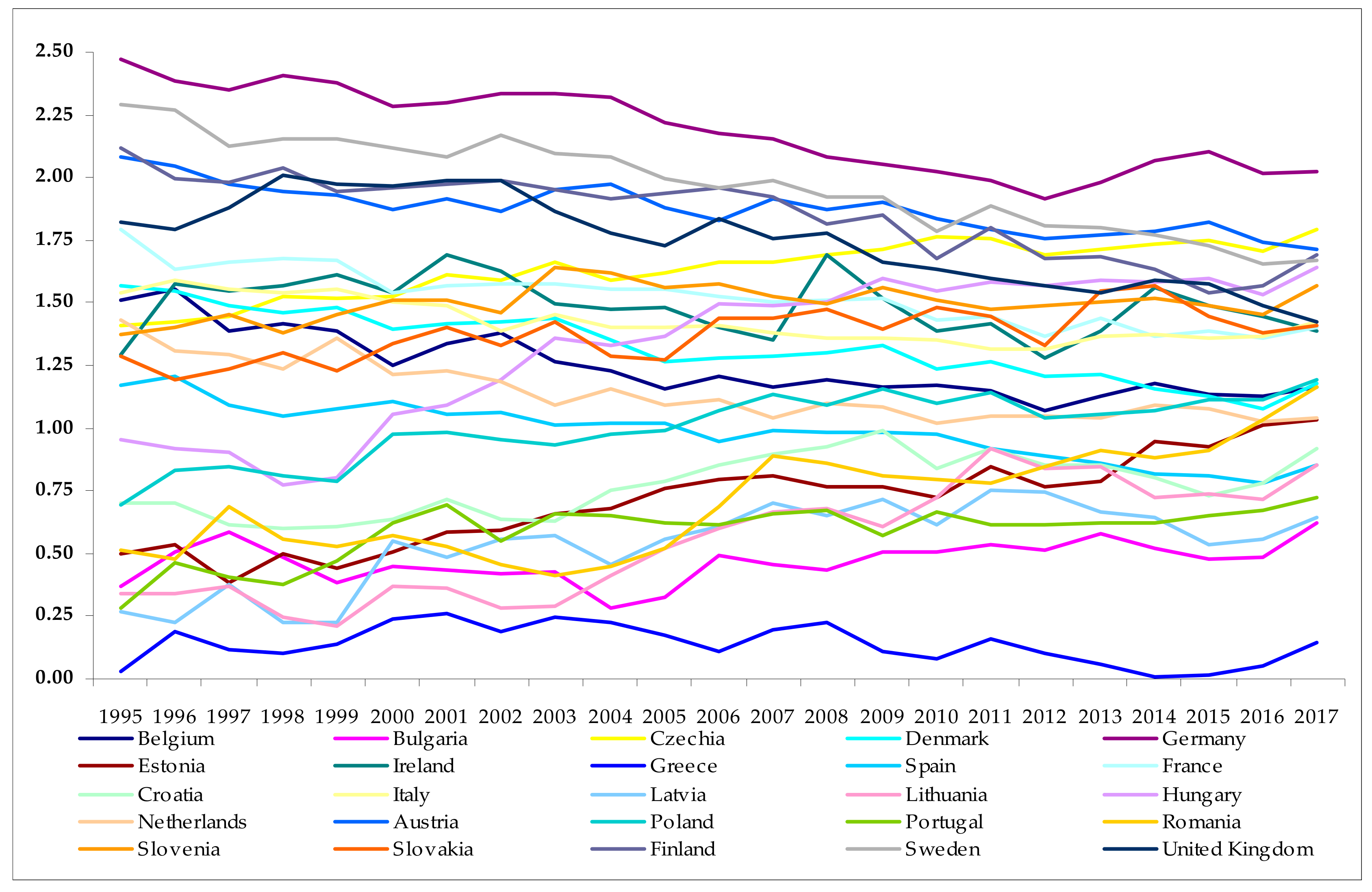
The values of ECI range from 0.093 (Greece) to 2.474 (Germany) in the examined period of time. We notice a group of 11 countries (Germany, Sweden, Finland, Austria, United Kingdom, France, Spain, Denmark, Belgium, Italy and Netherlands), where ECI decreases continuously from 1995 to 2017. The sharpest declines (in 2017 compared to 1995) were registered in Netherlands (27%) and Denmark (25%) and the smallest in Italy (7.2%). These are the most prosperous and largest export economies in the European Union and even in the world. For example, Germany is the 2nd largest exporter in the world and the 3rd most complex economy; Sweden, Finland and Austria are also among the ten most complex economies in the world in 2017 [93]. There is a group of four countries (Ireland, Slovakia, Czech Republic and Slovenia) where ECI ranges from 1.25 to 1.45 in 1995 and the increase of ECI is from 7–14% from 1995–2017. Another group of nine countries, with ECI values of 0.25 to 1 (Hungary, Croatia, Poland, Romania, Estonia, Bulgaria, Lithuania, Portugal and Lithuania), has a strong ascending trend. Portugal recorded the highest increase, with 158.23%, followed by Lithuania (149.70%), Latvia (139.94%), Romania (126.03%) and Estonia (107.11%). Moderate growth can be observed in Hungary (72.32%), Poland (71.76%), Bulgaria (70.40%) and Croatia (30.51%). Greece is a special case, with the lowest level of ECI in the examined period of time and a slight increase (of 11.80%) (Figure 1).

Based on the above assertions, a pattern of ECI dynamics could be identified: countries with higher income and higher start of ECI in 1995 (1.45–2.5) have a decreasing evolution. At a medium level of ECI (1.25–1.4), a slight increasing trend is noticed and when the values of ECI range from 0.25 to 1 the increasing trend is stronger, the growth being higher than in all cases.

According to Hausmann et al. (2011) [2], economic complexity is related to a country’s level of prosperity, it is not only a symptom of prosperity, it is a driver. Moreover, economic complexity can explain differences in the level of income of countries and can predict future economic growth.

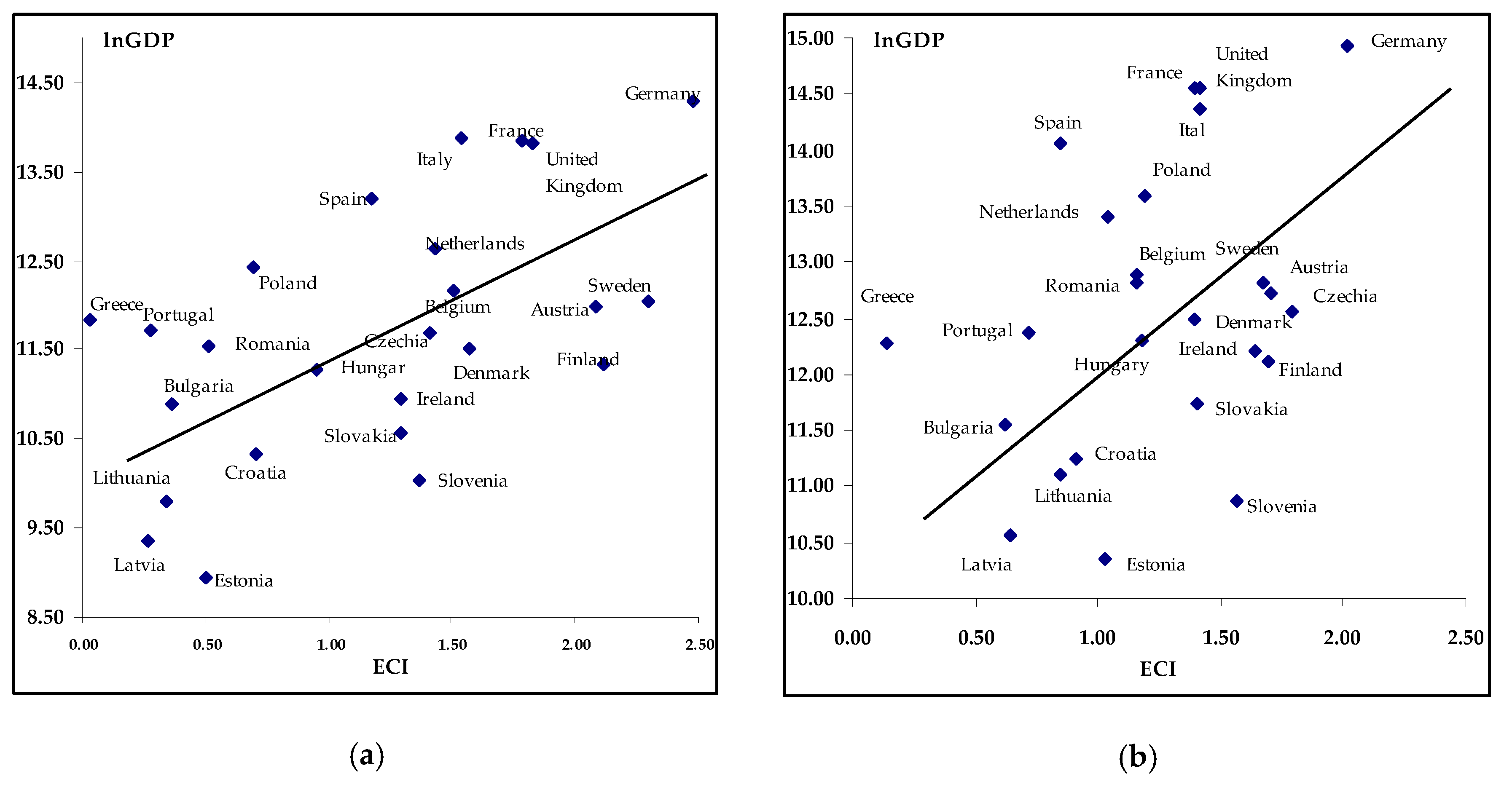
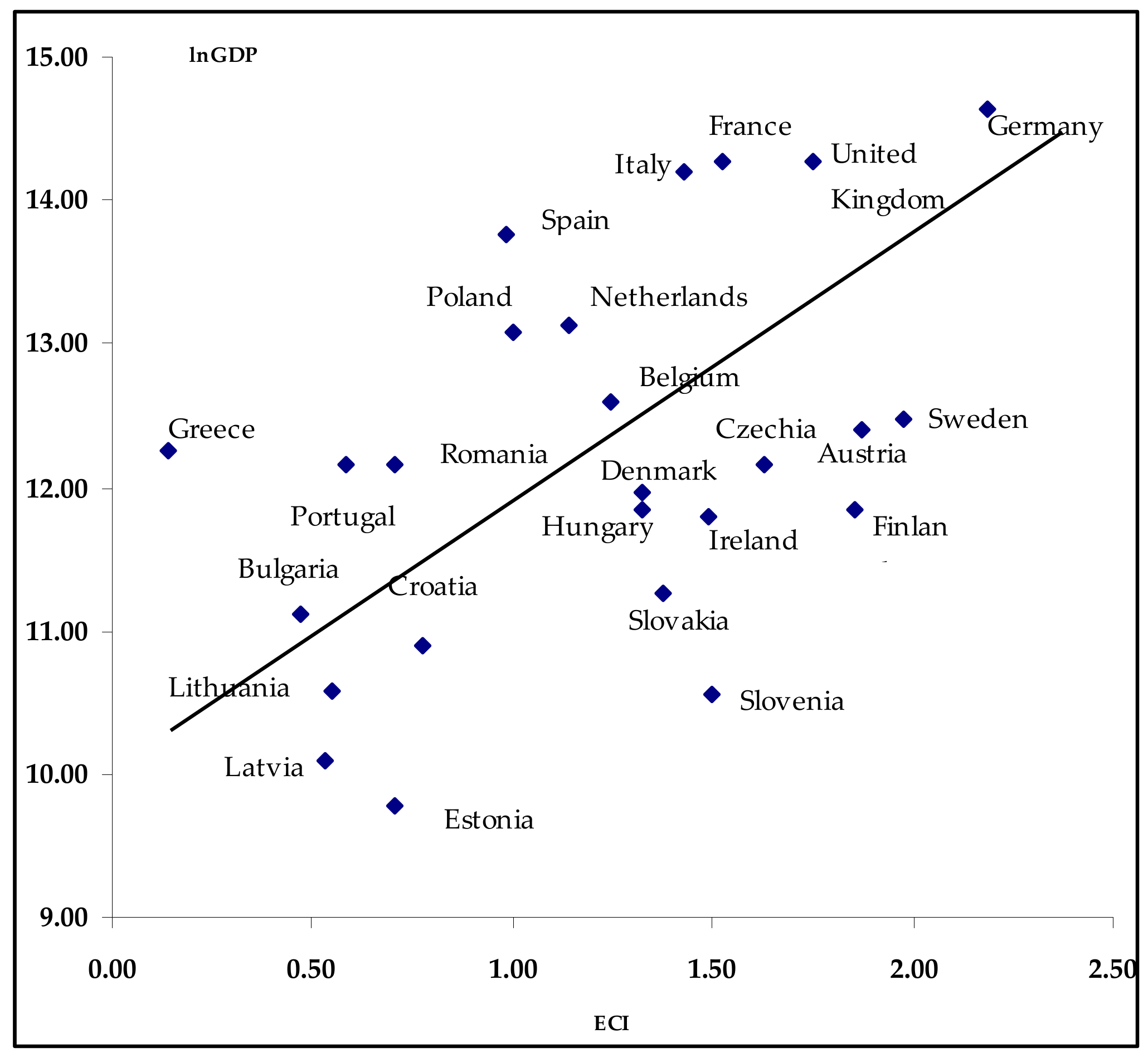
Figure 2 displays the graphical dependency between lnGDP and ECI in the sample of 25 EU economies (average values for 1995–2017). We notice that countries are spread on both sides of the regression line, illustrating the positive correlation between the two variables.

The correlation between lnGDP and ECI is positive and strong to moderate in the time span 1995 to 2017 (Figure 3a,b). In 1995, the correlation coefficient of lnGDP and ECI is 0.56, higher than in 2017 when it is 0.38. This positive association between the two variables indicates us that ECI could be used instead of lnGDP in the EKC model.

2.4. Econometric Specifications

2.4.1. Panel Data

Model

We adopt the following model (Equation (3)) to be tested:

$$\ln CO{2}_{it}={\alpha }_i+\delta \cdot t+{\beta }_{1i}\cdot EC{I}_{it}+{\beta }_{2i}\cdot EC{I}_{it}^2+{\beta }_{3i}\cdot \ln E{I}_{it}+{\mu }_{it}$$

(3)

where t is a linear time trend, ${\beta }_{1i}$${\beta }_{2i}$${\beta }_{3i}$ are elasticities of lnCO₂ as regards to ECI, $EC{I}^2$ and respectively to EI and ${\mu }_{it}$ is the error term. Given that ECI may follow an integrated process integrated of order one, the above relationship (3) is a cointegrating polynomial regression (CPR) if ${\mu }_{it}$ is stationary [69]. Furthermore, given the panel nature of data, it is reasonable to believe that the error terms are heteroskedastic and cross-sectionally dependent.

The following situations are possible: (i) ${\beta }_1={\beta }_2=0$ indicates that CO₂ is not related to ECI (ii) ${\beta }_1$ > 0 and ${\beta }_2=0$ refers to a monotonically increasing relationship between CO₂ and ECI, (iii) ${\beta }_1$ < 0 and ${\beta }_2=0$ reflects a monotonically decreasing relationship between CO₂ and ECI, (iv) ${\beta }_1$ < 0 and ${\beta }_2$ > 0 specifies a U-shaped relationship between CO₂ and ECI and (v) ${\beta }_1$ > 0 and ${\beta }_2$ < 0 expresses an inverted U-shaped relationship between CO₂ and ECI. According to EKC hypothesis, we expect to obtain ${\beta }_1$ > 0 and ${\beta }_2$ < 0. The expected sign of ${\beta }_3$ is positive since energy intensity leads to higher pollution [50,66,94].

The methodology used in this paper consists of the following steps: (1) cross-sectional dependence is tested; (2) stationarity of variables is checked through panel unit root test; (3) the long-run relationship between variables is tested with the panel cointegration method; (4) if the cointegration is confirmed, the regression coefficients are estimated with panel fully modified ordinary least square (FMOLS) and dynamic ordinary least square (DOLS) methods and (5) stationarity, cross-sectional dependence (as suggested by Müller-Fürstenberger and Wagner, 2007) [68] and ratio variance of errors is tested.

Cross-Sectional Dependence

Due to the nature of a panel including 25 EU countries, we may believe that cross-sectional dependence is possible, as a result of the EU membership the EU common policies.

We will test the cross-sectional dependence through the following tests: Breusch–Pagan LM (1980) [95], Pesaran scaled LM and Pesaran CD (2004) [96].

Based on Pesaran’s (2004) [96] assertion, the null hypothesis of no cross-sectional dependence implies that the correlation of disturbances between different cross-sections (countries) is zero, while the alternative states that this correlation is different from zero. According to the Breusch–Pagan (1980) [95] Lagrange Multiplier (LM) test, the LM statistic calculates correlation coefficients obtained from residuals and chi-squared distribution, under a normality assumption of errors. Pesaran (2004) [96] proposed first a standardized version of LM statistic, the scaled LM, appropriate for large number of cross-sections. Furthermore, Pesaran (2004) [96] introduced, an alternative test, called CD statistic, based on the average of the pairwise correlation coefficients. In all cases, when applying these tests, the values of Prob under 0.05 will indicate the rejection of null hypothesis of no cross-section dependence.

Stationarity of Data

To check the stationarity of panel data series we use the tests introduced by Levin, Lin and Chu (LLC) (2002) [97], Im, Pesaran and Shin (IPS) [98] and Maddala and Wu (1999) [99].

In testing the stationarity of panel data, an autoregressive AR (1) process across sections is considered (Equation (4)):

$$y_{it}={\rho }_i{y}_{it-1}+x_{it}{\delta }_i+{\epsilon }_{it}$$

(4)

where i denotes the cross-sections and t the time, y_it is the dependent variable, x_it represent the exogenous variables, ρ_i is the vector of autoregressive coefficients and ε_it represent the errors.

If |ρ_i| = 1, then y_i contains a unit root. If ρ_i = ρ, for all i, then the parameters are common across all cross-section. Under this assumption Levin, Lin and Chu (LLC) (2002) [97] introduced a unit root test based on the following Equation (5).

According to Levin, Lin and Chu (LLC) [97] test, a common and identical unit root process can be identified across cross-sections. The panel unit root tests are based on Equation (5):

$$\Delta y_{it}=\alpha \cdot y_{it-1}+{\displaystyle \sum _{j=1}^{p_i}{\beta }_{ij}}\cdot \Delta y_{it-j}+{X^{\prime }}_{it}\cdot \delta +{\epsilon }_{it}$$

(5)

where α is common for all cross-sections and the lag order for difference terms p_i may vary across cross-sections. The null hypothesis of the presence of the unit root is given by α = 0, while the alternative by α < 0.

The test developed by Im, Pesaran and Shin (2003) [98] allows individual unit root processes, meaning that the parameters can vary across cross-sections and separate regression Equation (5) is conducted in each cross-section. The null hypothesis is the result of α = 0 for all 1, and respectively, the alternative α_i = 0 for i = 1, 2, …, N₁; α < 0 for i = N + 1, N + 2, …, N.

The Fisher-ADF test proposed by Maddala and Wu (1999) [99] combines the p-values from unit root test for each cross-section. The test is given by Equation (6):

$$\lambda =-2{\displaystyle \sum _{i-1}^n{\log }_e}\left(p_i\right) ~{\chi }_{2n(d.f.)}^2$$

(6)

where ${\chi }_{2n(d.f.)}^2$ is the chi-square distribution with 2n degrees of freedom, n is the number of countries in the panel, $p_i$ is the p-value from the ADF unit root test for the section i.

Panel Cointegration Test

We use the panel cointegration test developed by Pedroni (1999, 2004) [100,101] in order to find if the variables are cointegrated in the long run. Within this test, seven different test statistics are run. The null hypothesis of no cointegration (long-run) relationship can be rejected if the number of statistics with values of Prob under the selected significance level (1%, 5% or 10%) is at least 4 of 7. It means that a long-term relationship between the variables is identified.

Estimation of Long-Run Parameters

After identification of a long-run relationship, the cointegration coefficients will be estimated through the panel fully modified ordinary least squares (FMOLS) and the panel dynamic ordinary least squares (DOLS) methods developed by Pedroni (2001) [102,103].

The panel FMOLS Equations (7) and (8) are given by:

$$y_{it}={\alpha }_{it}+{\delta }_{it}t+\beta \cdot x_{it}+{\mu }_{it}$$

(7)

$$x_{it}=x_{it-1}+e_i$$

(8)

where $y_{it}$ is the dependent variable and $x_{it}$ denotes the independent variable, ${\alpha }_{it}$ represents the constant effects, $\beta$ is the long-term cointegration coefficient/vector.

The panel FMOLS estimator is specified in Equation (9):

$${\widehat{\beta }}_{FM}^{\ast }=n^{-1}{\displaystyle \sum _{i=1}^n{\widehat{\beta }}_{FM,i}^{\ast }}$$

(9)

where ${\widehat{\beta }}_{FM}^{\ast }$ is the FMOLS estimator applied to i-th section.

The associated T-statistic ($t_{{\widehat{\beta }}_{FM}^{*}}^{*}$) is calculated by Equation (10):

$$t_{{\widehat{\beta }}_{FM}^{*}}^{*}=n^{-1}{\displaystyle \sum _{i=1}^n{t}_{{\widehat{\beta }}_{FM,i}^{*}}}$$

(10)

The panel DOLS method introduced by Pedroni [104] is specified by Equation (11):

$$y_{it}={\alpha }_i+{\beta }_i{x}_{it}+{\displaystyle \sum _{k=-K_i}^{K_i}{\gamma }_{it}}\Delta x_{it-K}+{\epsilon }_{it}$$

(11)

This equation is estimated for each cross-section of the panel and then the cointegration coefficient for the overall panel is calculated as average of the DOLS coefficients for each section.

The panel DOLS estimator is calculated as in Equation (12):

$${\widehat{\beta }}_D^{\ast }=n^{-1}{\displaystyle \sum _{i=1}^n{\widehat{\beta }}_{D,i}^{\ast }}$$

(12)

The T-statistic follows as in Equation (13):

$$t_{{\widehat{\beta }}_D^{*}}^{*}=n^{-1}{\displaystyle \sum _{i=1}^n{t}_{{\widehat{\beta }}_{D,i}^{*}}}$$

(13)

Errors Tests (Stationarity, Cross-Sectional Dependence and Variance Ratio)

We check the stationarity of errors with LLC (2002) and IPS (2003) tests. The cross-sectional dependence of residuals will be examined with Breusch-Pagan LM [95], Pesaran and Pesaran CD [96] tests. For panel data series, the heterogeneous Lo and MacKinlay (1988, 1989) [104,105] variance ratio test will be performed. It is a variance ratio test for homoskedastic and heteroskedastic random walks of errors, using the asymptotic normal distribution [104] or wild bootstrap [106] to evaluate statistical significance. Lo and MacKinlay (1988, 1989) [104,105] assume that errors are independent and identically distributed (i.i.d) Gaussian with variance (the normality of errors is not strictly necessary), termed as homoskedastic random walk hypothesis. Alternatively, the heteroskedastic random walk hypothesis allows for conditional heteroskedasticity and dependence, termed as the martingale null. Under the assumption that cross-sections are independent, with cross-section heterogeneity of the processes, separate joint variance ratio tests are computed for each cross-section, then the p-values from cross-section are combined under the Fisher approach. When the joint combined Fisher test displays a value of Prob corresponding to the max|z| statistic above the statistical significance threshold (1% or 5%) this indicates the acceptance of the null hypothesis of a martingale sequence of errors. All tests will be run for both equations (FMOLS and DOLS).

2.4.2. Country Data

For individual country data, the following Equation (14) will be estimated:

$$\ln CO{2}_t=c+\delta \cdot t+{\beta }_1\cdot EC{I}_t+{\beta }_2\cdot EC{I}_t^2+{\beta }_3\cdot \ln E{I}_t+{\mu }_t$$

(14)

Both FMOLS and DOLS equations will be estimated for each of 25 examined countries and the statistical validity of coefficients is inspected. For the cases where the coefficients are statistically validated for, at least 5% significance, the cointegrating polynomial regression with ECI and $EC{I}^2$ as regressors is estimated (Equation (15)).

$$\ln CO{2}_t=C+\delta \cdot t+{\lambda }_1\cdot EC{I}_t+{\lambda }_2\cdot EC{I}_t^2+{\mu }_t$$

(15)

The following steps are run: (1) the cointegration of regressors ECI and $EC{I}^2$ is tested; (2) the coefficients of FMOLS and DOLS regressions are estimated and their statistical validity is examined, and (3) stationarity of errors is verified, as well as their variance ratio.

As suggested by Wagner (2015) [70], in a cointegrating polynomial regression, the cointegration of regressors must be checked; the Johansen methodology (1991) [107] will be used in this view.

The FMOLS equation is based on Phillips and Hansen (1990) [108] estimator which employs semi-parametric correction to avoid the problems caused by the long-run correlation between the cointegrating equation and stochastic regressor innovation. The DOLS method involves augmenting the cointegrating regression with lags and leads of differenced regressors and results the orthogonality of error term to the stochastic regressor innovation [109,110].

For testing the errors stationarity, the Philips-Ouliaris (1990) [111] test is employed. It is a residual-based test for cointegration or a simple unit root test applied for residuals obtained from an OLS equation estimation. The null hypothesis of the presence of unit root in the residuals is rejected when the value of Prob is lower than the chosen significance threshold (1% or 5%), while the alternative states the stationarity of the residuals series.

The Lo and MacKinlay (1988, 1989) [104,105] variance ratio test described above will be performed in order to explore the martingale feature of errors in each case, the interpretation of max|z| statistic being similar.

3. Results

3.1. Results Based on Panel Data

3.1.1. Cross-Sectional Dependence Test

Table 2. Cross-sectional dependence test results.

Test	lnCO2		ECI		$\mathit{E}\mathit{C}{\mathit{I}}^2$		lnEI
	Statistic	Prob.	Statistic	Prob.	Statistic	Prob.	Statistic	Prob.
Breusch-Pagan LM	2639.244	0.0000	3311.269	0.0000	3265.325	0.0000	5704.11	0.0000
Pesaran scaled LM	95.499	0.0000	122.934	0.0000	121.058	0.0000	220.621	0.0000
Bias-correctedscaled LM	94.93	0.0000	122.366	0.0000	120.490	0.0000	220.056	0.0000
Pesaran CD	42.20	0.0000	-0.469	0.6332	-0.725	0.4654	75.129	0.0000

presents the results of cross-sectional independence test for the examined variables. As we can notice, the value of Prob is higher than 0.0000 only for two variables (ECI and $EC{I}^2$) for the Pesaran CD test. In other cases the value of Prob is 0.0000, leading us to reject the null hypothesis of cross-sectional independence and indicating the presence of cross-sectional dependence, as expected.

3.1.2. Stationarity of Data

Table 3. Panel unit root test.

Variable	LLC (a)		IPS		Fisher-ADF
	Intercept	Intercept and Trend	Intercept	Intercept and Trend	Intercept	Intercept and Trend
lnCO2	0.083	−2.210 (c)	1.189	0.332	50.073	43.140
ECI	−2.602 (b)	−1.926 (c)	0.402	−1.746 (c)	44.335	67.271 (b)
$EC{I}^2$	−2.551 (b)	−1.672 (c)	0.332	−2.099 (c)	46.464	74.286 (b)
lnEI	−3.040 (b)	−1.641 (c)	2.012	−1.939 (c)	33.657	64.806
ΔlnCO2	−7.178 (b)	−3.793 (b)	−9.569 (b)	−6.940 (b)	190.230 (b)	143.334 (b)
ΔECI	−9.0398 (b)	−6.398 (b)	−14.044 (b)	−11.673 (b)	273.864 (b)	214.388 (b)
Δ$EC{I}^2$	−8.130 (b)	−5.406 (b)	−13.962 (b)	−11.651 (b)	271.901 (b)	214.538 (b)
Δ lnEI	−9.009 (b)	−6.506 (b)	−10.267 (b)	−7.464 (b)	198.341 (b)	142.114 (b)

Notes: (a) Newey-West bandwidth selection with Bartlett Kernel is used for LLC test. (b) Illustrates 1% statistical significance. (c) Illustrates 5% statistical significance.

depicts the panel unit root test results. We notice that the series of variables at level value are not stationary, for all three tests, meaning that they are integrated at the first order for a 1% level of significance.

3.1.3. Panel Cointegration Results

Table 4. Pedroni panel cointegration test.

Test	Statistic	Prob.	Statistic	Prob.
Common AR Coefficients (within-Dimension)
Panel v-statistic	0.390487	0.3481	−0.754742	0.7748
Panel rho-statistic	−1.427714	0.0767	−2.767018	0.0028
Panel PP-statistic	−4.387047	0.0000	−7.327976	0.0000
Panel ADF-statistic	−3.598100	0.0002	−5.145805	0.0000
Individual AR Coefficients (between-Dimension)
Panel rho-statistic	−0.849445	0.1978
Panel PP-statistic	−8.159586	0.0000
Panel ADF-statistic	−4.558682	0.0010

Note: Newey-West Bandwidth selection with Bartlett Kernel is used, under the assumption of deterministic intercept and trend.

exhibits the panel cointegration results. One may observe that 6 out of 7 statistics have their corresponding value of Prob. under 0.05, indicating a valid cointegration relationship between lnCO₂, ECI, $EC{I}^2$ and lnEI.

3.1.4. Estimation of Long-Run Parameters

As we can notice in

Table 5. Panel cointegration coefficients.

	Panel FMOLS (a)			Panel DOLS (a)
	ECI	$\mathit{E}\mathit{C}{\mathit{I}}^2$	lnEI	ECI	$\mathit{E}\mathit{C}{\mathit{I}}^2$	lnEI
Panel	0.552 (b)	−0.124 (b)	0.393 (b)	0.625 (b)	−0.173 (b)	0.372 (b)
	[4.655]	[−2.787]	[10.488]	[3.538]	[−2.596]	[6.713]
R-squared	0.9954			0.9978
Number of observations	575

(a) The values in brackets are t-statistics. (b) Illustrates 1% level of significance.

, the cointegration coefficients are validated within the panel, for both (FMOLS and DOLS) estimations, for a 1% level of significance. A quadratic dependency between lnCO₂ and ECI in the long run is validated, indicating an inverted U-shaped curve. The coefficient of ECI is positive (0.552; 0.625) and of $EC{I}^2$ is negative (−0.124; −0.173). The effect of energy intensity (lnEI) is also positive and statistically significant on lnCO₂; for a rise of 10% of energy intensity, carbon emissions increase with 3.93% (FMOLS estimation), respectively 3.72% (DOLS estimation).

3.1.5. Errors Test (Stationarity, Cross-Sectional Dependence and Variance Ratio)

As decided in the previous section, we check the stationarity of errors in order to obtain a validation of the polynomial regression. According to the results of the unit root tests (

Table 6. Stationarity test for FMOLS and DOLS equations residuals.

	LLC		IPS
	Intercept	Intercept and Trend	Intercept	Intercept and Trend
FMOLS resid	−2.21 (b)	−2.88 (a)	−1.78 (b)	−1.70 (b)
DMOLS resid	−2.27 (b)	−2.53 (b)	−2.23 (a)	−1.29 (b)

(a) Illustrate 1% level of significance. (b) Illustrate 5% level of significance.

), the residuals of FMOLS and DOLS estimated equations follow a stationary trend for a 5% level of significance.

Furthermore, when checking the errors’ cross-correlation with Breusch-Pagan, Pesaran scaled LM and Pesaran CD tests, the results reveal the presence of cross-sectional dependence of residuals (the value of Prob is 0.000) (

Table 7. Cross-section dependence test of panel FMOLS and DOLS equations residuals.

Test	FMOLS		DOLS
	Statistic	Prob	Statistic	Prob
Breusch–Pagan LM	988.197	0.0000	988.151	0.0000
Pesaran scaled LM	28.095	0.0000	27.930	0.0000
Bias-corrected scaled LM	27.526	0.0000	27.272	0.0000
Pesaran CD	3.404	0.0023	18.616	0.0000

).

As one may notice from

Table 8. Variance ratio test of panel FMOLS and DOLS equations’ residuals.

	FMOLS		DOLS
Fisher Combined Test	$\mathbf{max} \left|\mathit{z}\right|$	Prob.	$\mathbf{max} \left|\mathit{z}\right|$	Prob.
asymptotic normal	151.571	0.000	32.483	0.9740
wild bootstrap	73.666	0.000	27.412	0.9961

, the null hypothesis of a martingale residual series is strongly rejected in the case of panel FMOLS equation (Prob is 0.0000) and accepted in for the panel DOLS estimator (Prob is above 5%). This means that error series follows a martingale sequence for DOLS equation, and the expected next value in the errors sequence is equal to the present value.

We may conclude now that within the panel analysis, in the presence of cross-sectional dependence, the cointegrating polynomial regression is validated, according to the findings of Wagner and Hong (2016) [71], and reflects the quadratic dependence of carbon emissions of economic complexity when the variable “energy intensity” is included.

3.2. Results Based on Country Data

As a result of regression coefficients estimation conducted for the 25 individual countries (see Appendix A), the quadratic model is validated only for ten countries: Belgium, Greece, Spain, France, Italy, Hungary, Slovenia, Finland, Sweden and the United Kingdom. In Belgium, France and Italy the coefficients for both FMOLS and DOLS equations are validated for 1% significance. For Hungary only the FMOLS estimation is validated for 1% significance and in Slovenia, only DOLS estimation can be validated for 5% significance. In Finland the coefficients of both estimators are validated and in Sweden, all coefficients are validated for 5% significance level.

As decided above, we test the cointegration of regressors (ECI and $EC{I}^2$) and estimate the cointegrating polynomial regression (15) for the ten countries (see

Table 9. Cointegration test of regressors and estimation of FMOLS and DOLS coefficients for Equation (15).

Country	Johansen Test (Trace Statistics)	FMOLS			DOLS
		ECI	$\mathit{E}\mathit{C}{\mathit{I}}^2$	C	ECI	$\mathit{E}\mathit{C}{\mathit{I}}^2$	C
Belgium	39.356 (a)	6.862 (a)	−2.419 (a)	6.938 (a)	15.675 (a)	−5.886 (a)	1.368 (a)
Greece	14.636 (b)	3.470 (b)	−6.290 (b)	11.173 (a)	5.864 (a)	−14.064 (b)	11.037 (a)
Spain	26.664 (a)	13.874 (a)	−6.993 (a)	5.859 (a)	18.695 (a)	−9.478 (a)	3.546
France	38.504 (a)	11.653 (a)	−3.624 (a)	3.648 (b)	11.946 (a)	−3.697 (a)	3.355 (b)
Italy	19.787 (b)	22.813 (a)	−8.262 (a)	−2.385 (b)	24.699 (a)	−8.909 (a)	−3.702
Hungary	24.674	2.405	−1.119	9.785 (a)	2.137 (a)	−1.101 (a)	9.924 (a)
Slovenia	18.458 (b)	2.851	−1.335	9.214 (b)	15.623 (a)	−6.050 (a)	0.619
Finland	18.356 (b)	9.905 (a)	−2.559 (b)	1.489 (b)	11.961 (b)	−3.113	−0.406
Sweden	18.660 (b)	1.978	−0.364	8.412 (a)	3.448 (b)	−0.743 (b)	6.999 (b)
United Kingdom	20.540 (b)	6.944 (a)	−1.824 (a)	6.704 (a)	8.000 (a)	−2.115 (a)	5.750

(a) Illustrate 1% level of significance. (b) Illustrate 5% level of significance.

). The first column displays the value of trace statistic of Johansen test. One may notice that in all cases, except Hungary, the values of trace statistic, displayed in the first column, indicate at least one cointegration relationship. We also notice from columns 2–7 that in only eight cases the coefficients of regressors (ECI and $EC{I}^2$) are statistically validated. In Belgium, Greece, France and Italy the coefficients of both equations (FMOLS and DOLS) are validated, in Spain, Finland and United Kingdom only those of FMOLS estimator and in Sweden for DOLS estimation.

In the next step of testing stationarity of errors with Phillips-Ouliaris test (first column of

Table 10. Residuals test for the ten EU countries (stationarity and variance ratio test).

Country	Phillips-Ouliaris Test (Tau Statistic)	Variance Ratio Test (Fisher Test)
		FMOLS		DOLS
		$\mathbf{max} \left|\mathit{z}\right|$	Prob.	$\mathbf{max} \left|\mathit{z}\right|$	Prob.
Belgium	−3.980 (b)	1.452	0.4691	0.482	0.9812
Greece	−3.353	1.641	0.3459	1.237	0.6220
Spain	−2.919	0.625	0.9519	1.177	0.6646
France	−5.673 (a)	2.306	0.0817	1.432	0.6885
Italy	−4.852 (b)	0.599	0.9587	1.953	0.099
Hungary	−2.407	1.967	0.182	1.344	0.545
Slovenia	−3.448	1.888	0.215	2.100	0.135
Finland	−4.477 (b)	1.713	0.303	1.355	0.537
Sweden	−5.579 (a)	1.292	0.582	1.773	0.271
United Kingdom	−3.829 (b)	1.753	0.282	1.458	0.464

(a) Illustrate 1% level of significance. (b) Illustrate 5% level of significance.

), Greece, Spain, Hungary and Slovenia are excluded due to the values of tau statistic for 1% or 5 significance level. For the six remained countries (Belgium, France, Italy, Finland, Sweden and United Kingdom) the results of the variance ratio test for FMOLS and DOLS residuals (columns 2–5 of Table 10) indicate that the residuals have characteristics of a martingale sequence. According to Wagner and Hong (2016), the conditions for the validation of a cointegrating polynomial regression in these six cases (cointegration of regressors, stationarity and martingale characterization of errors) are fulfilled.

4. Discussion

The paper validates a model predicting a quadratic dynamics of carbon emissions depending on the economic complexity in a panel of 25 countries through a cointegrating polynomial regression, as defined by Wagner and Hong (2016) [71]. For the first time in the existing literature of EKC, the variable “income” as main determinant of pollution, was replaced by economic complexity in a panel data framework. The model is also tested for simple time series, in 25 individual economies.

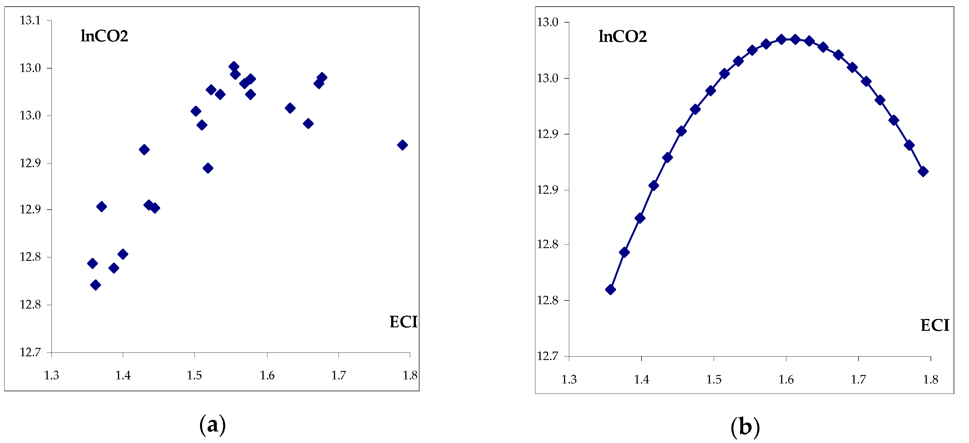
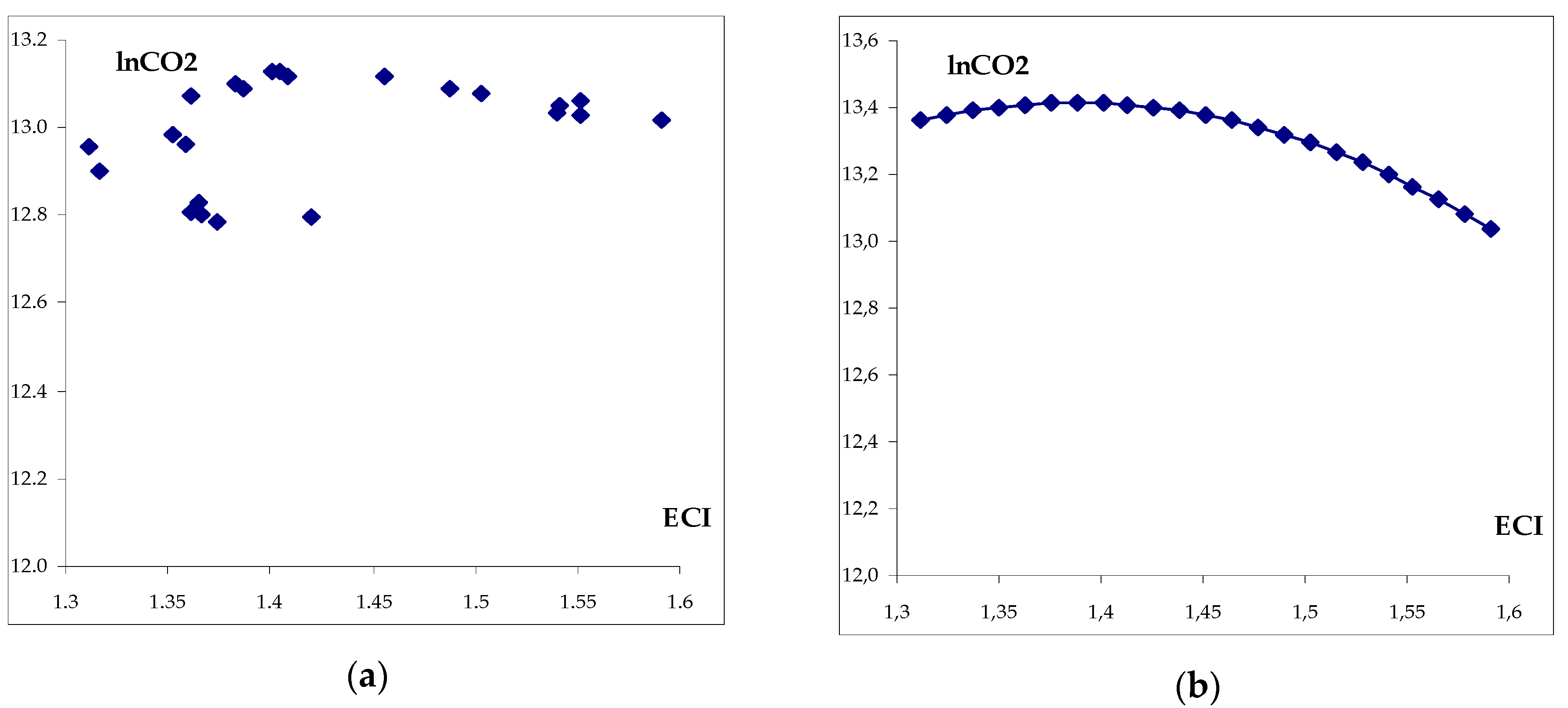
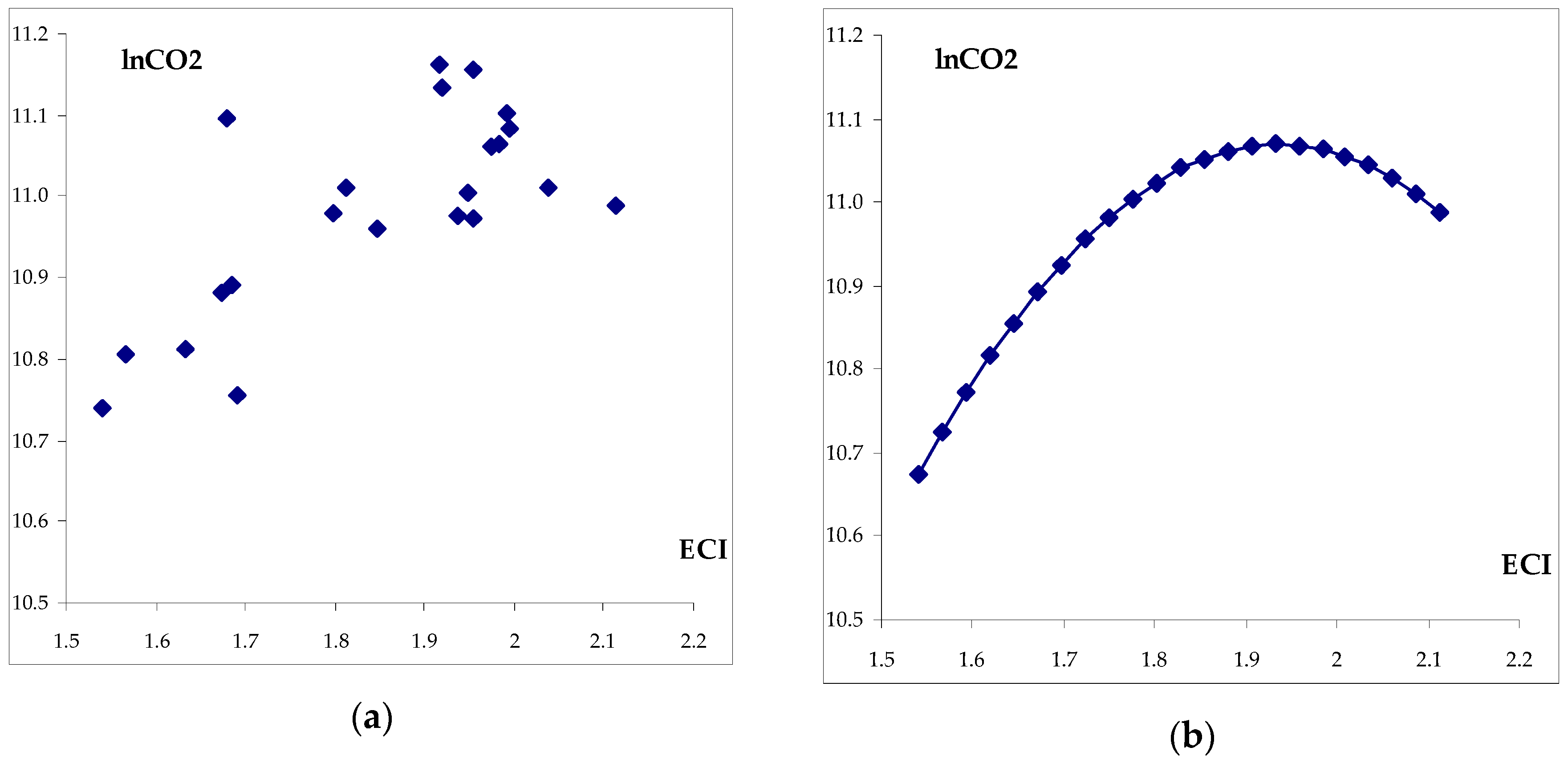
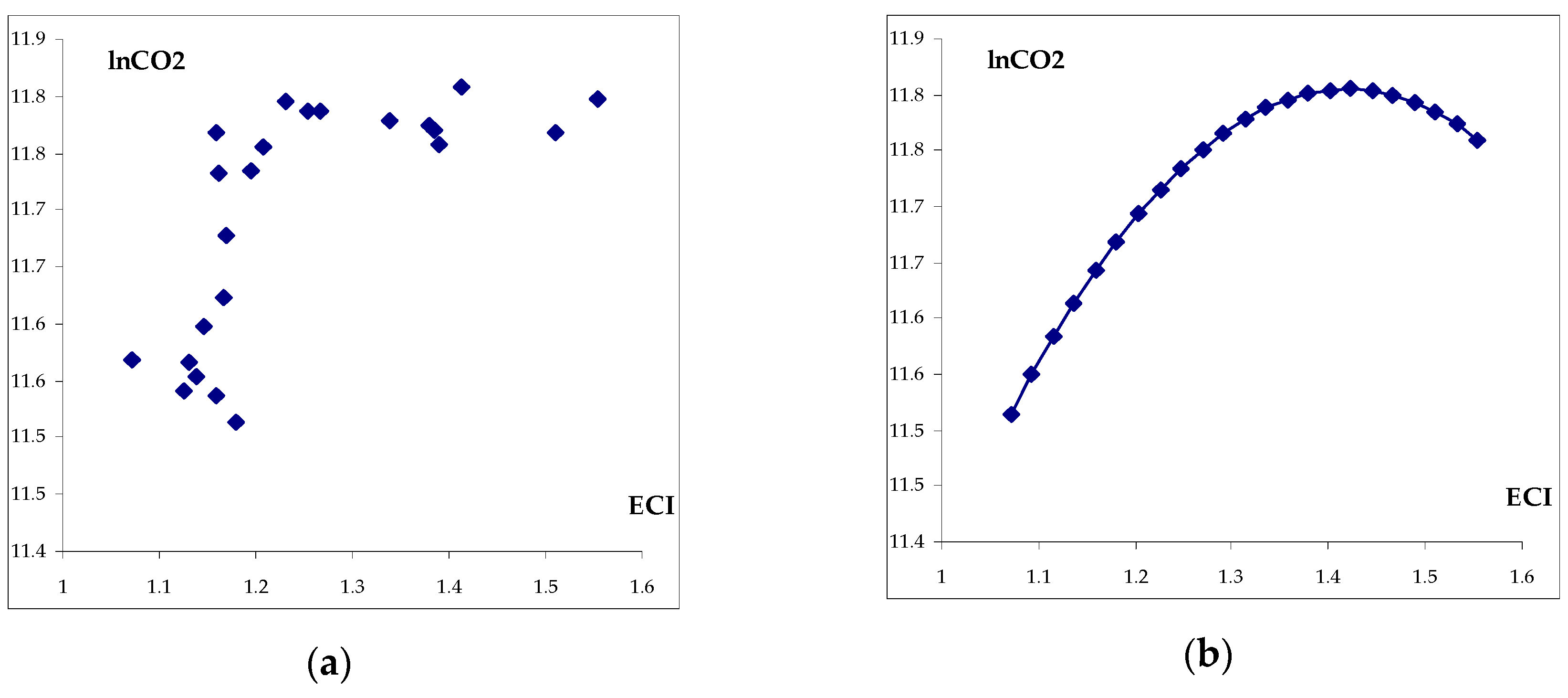
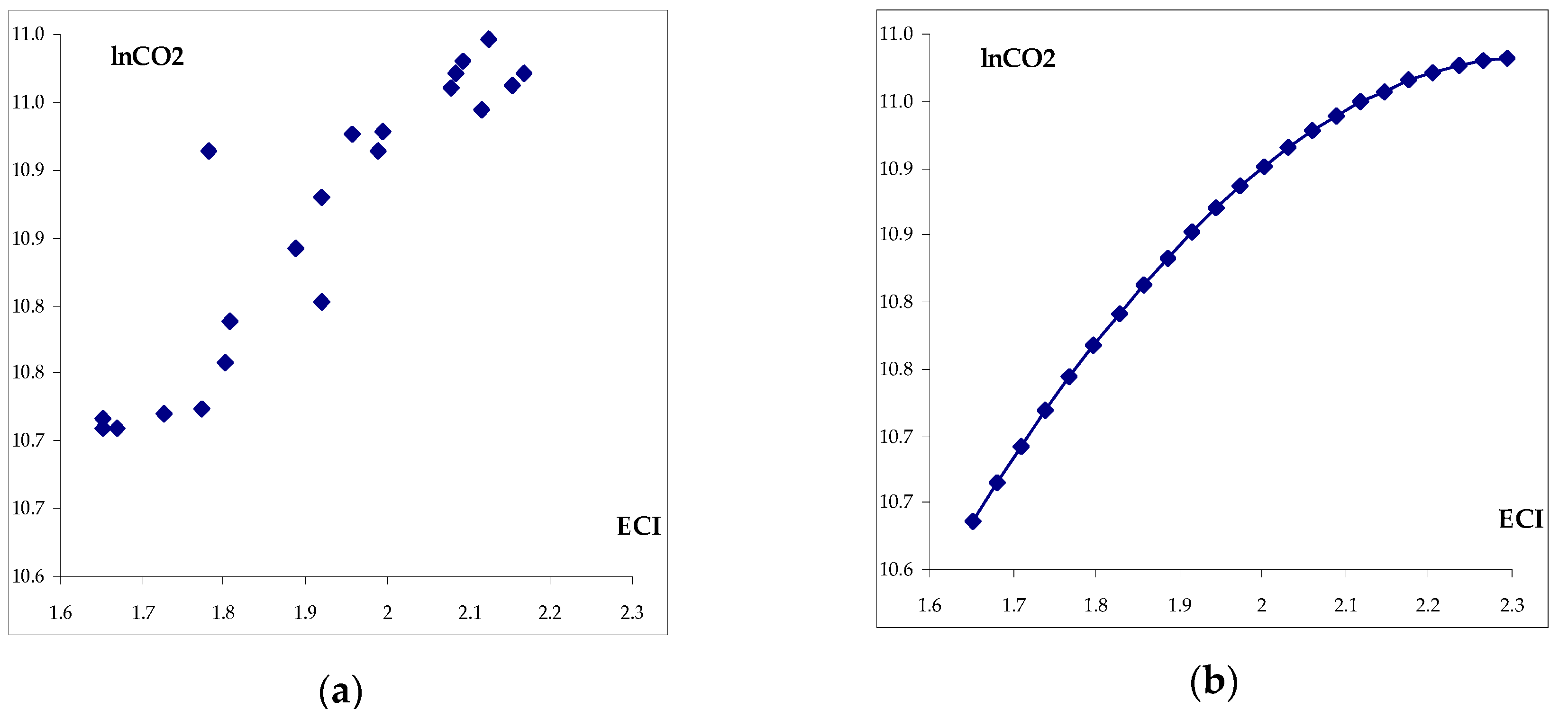
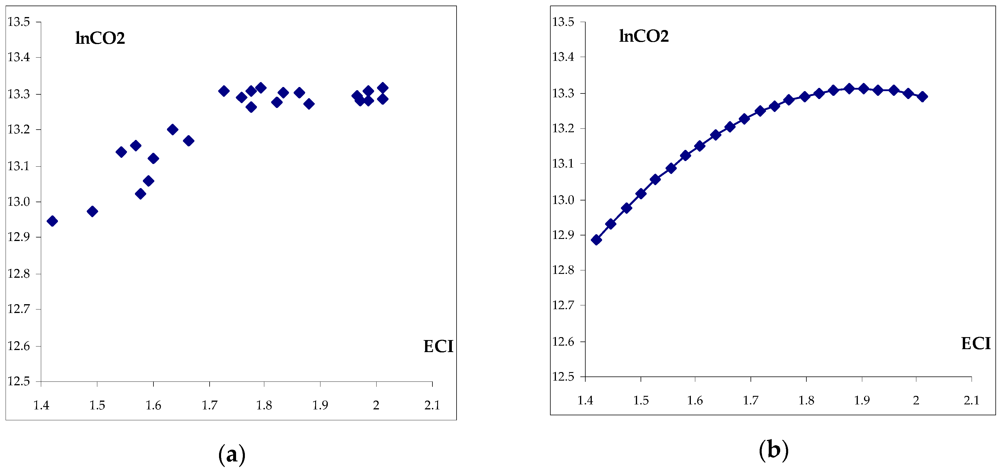
The estimation results for the six validated cases (Belgium, France, Italy, Finland, Sweden and the United Kingdom) in Table 9, are displayed graphically in Figure 4, Figure 5, Figure 6, Figure 7, Figure 8 and Figure 9. The (a) version shows the dots of lnCO₂ and ECI observations for 1995–2017. The (b) version is the graphical representation of the analytical estimated EKC model for each country. The graphics resulted through the inserting equidistantly spaced points from the sample range of ECI, with corresponding values of the trend, using the estimated coefficients.

The estimated EKC for France exhibits a clearly inverted U-shape. The turning point corresponds to an ECI value around 1.6. As ECI increase above this level, the continual reduction of carbon emission is achieved. The allure of graph in the case of France suggests that there are three main periods in the dependency of pollution on ECI, similarly to pollution on income. In a first stage, the increase of economic complexity induces the rise of pollution. This is the period of extensive use of resources in order to sustain the complexity advance of exported products. It lasts until to a turning point, when the economic complexity shifts to the stage of efficiency and effectiveness in the use of resources and when more complex products are embedding sophisticated and less pollutant technologies. This stage reflects also a higher rate of return to investments in knowledge-intensive sectors, human capital and R&D and innovation activities related to energy production and manufacture industries.

The case of Italy is very different from other countries; the curve is slightly shaped as an inverted U. Even if the negative coefficient of $EC{I}^2$ is the highest of all cases (−8.28), due to the negative value of the constant term) (−2.38) the ascending stage is short and the turning point is less noticeable due to a little bit long stage of stationary trend of lnCO₂. When ECI becomes higher than 1.45, the downturn of lnCO₂ is more visible.

The estimated EKC curve for Finland is somehow similar to Belgium; the negative coefficient of $EC{I}^2$ has closed values (−2.41 in Belgium and −2.55 in Finland). The value of ECI corresponding to the curve’s turning point is different: in Finland the carbon emissions start to decrease when ECI reaches values higher than 1.9 and in Belgium when ECI attained 1.4.

Sweden and the United Kingdom evolve both in an ascending stage. The case of Sweden expresses an ascending line, with a very slight sign of stagnation of pollution when ECI is higher than 2.2. The graph of the United Kingdom shows that the economy is positioned on the descending stage of the dependency of carbon emissions on ECI. A slight decreasing stage with a low rate can be noticed due to the reduced value of the $EC{I}^2$’s coefficient (1.82).

What do these six EU economies have in common? We discuss below country features related to possible factors and developments that may enable the decreasing stage of CO₂ curve, when suppression of emissions is possible with the advance of economic complexity.

The countries for which the EKC model with economic complexity as explanatory variable was been validated are developed EU Member States, with high levels of economic complexity index (above 1) in the period of 1995–2017.

The export products basket of these countries mainly includes: refined petroleum (the United Kingdom, Sweden, Italy, Denmark and Finland), packaged medicaments (France, Belgium, Italy, Sweden and the United Kingdom), kaolin coated paper (Finland and Sweden), planes/helicopters/aircraft (France and United Kingdom), cars and vehicle parts (the United Kingdom, Sweden, Italy, France and Finland) [93]. The structure of exports indicates a specific development of chemical (refined petroleum, medicaments, and paper), manufacture (cars, machinery) and high tech-sectors, which are based on energy-intensive activities. The highest shares of high technology products in total exports in 2017 were reached in: France (20%), the United Kingdom (18.1%), Sweden (11.9%) and Belgium (10.3%) [112].

The competitiveness such products is based on high investments in R&D and human capital. According to EUROSTAT [113] the levels of R&D expenditures in these countries were in 2017 higher than the EU’s average (2.06% of GDP) (i.e., 3.4% in Sweden, 2.76% in Finland, 2.58% in Belgium and 2.19% in France). The share of human resources in science and technology (as % of active population) is also above the 2017 EU’s average of 46.6%: 58.6% Sweden, 57.7% Finland, 57% the United Kingdom, 54.3% Belgium and 50.8% France [114].

They also massively invest in innovation activities related to energy production. For example, the public funding for Energy Technology Research, Development and Demonstration (ETRDD) (as ratio of GDP) is the highest of the EU in Finland, France, Belgium, Sweden, Italy and the United Kingdom [115].

As a net importer of energy (coal, crude oil, oils products), Sweden has the highest share of renewable sources in the energy mix and an almost carbon-free electricity supply. It is integrated within the Nordic and Baltic electricity markets and developed a joint renewable certificate market with Norway, providing a unique model for other countries [116]. A similar situation of import dependency in Finland has driven to national targets of renewable sources to be set out above 50% for 2020s, the Finland’s industry on second generation bio-fuels is leading globally and the renewable sources in manufacturing sector reached almost 40% in 2016 [115,117]. France has a significant low-carbon electricity mix due to the key role of nuclear energy. Large investments in renewable energy and efficiency are planned while security of supply, low-carbon footprint and growth of renewable electricity are goals for the long-term [118]. Italy has made notable progress on renewable sources development, market liberalisation and infrastructure for electricity and also to become a southern European gas hub [119]. The participation of these countries to the EU STS scheme, a good platform of carbon market to electricity companies as assessed by Ji et al., 2019 [38], could partially explain the abatement of carbon emissions in these countries.

The United Kingdom is leading by example, as regarding the low-carbon investments in various technologies, carbon capture and storage technologies and electricity market reform [120]. A Clean Growth Strategy was set out as well as a Modern Industrial Strategy [121,122], which integrates a green growth perspective considered to be necessary to achieve economic and environmental goals and investment in low-carbon transformation. One of the five electric vehicles driven in Europe is made in the UK and more than 430,000 jobs were created in low-carbon business [122]. Belgium is committed to decarbonise the economy, by reducing the use of fossil fuels and increasing the use of renewable energy. In 2016 the nuclear energy accounted for around half of Belgium’s electricity generation [123].

5. Conclusions

The present paper provides a study of the EKC model, by replacing the log GDP per capita with economic complexity. As discussed, the presence of ECI power renders the usage of methods developed for linear cointegration problematic. We used therefore a cointegrating panel regression [70,71], which was estimated through heterogeneous panel techniques. The quadratic dependence between CO₂ emissions, economic complexity and energy intensity is identified in a panel of 25 EU countries. The analysis of individual countries revealed that for only six EU economies the EKC hypothesis based on cointegrating panel regression incorporating ECI is validated.

The main findings of the paper are the following. The long-run dependency between economic complexity and carbon emissions is illustrated as an inverted U-shaped curve, similarly to the EKC for income, and this is the novel contribution of the paper to the existing literature of EKC hypothesis. In a first period of economic complexity advance, the carbon emissions increase due to the extension of resources and activities embedded in more complex and sophisticated products. In a second stage, when the efficiency in diversifying exported products increases, the raise of economic complexity does not lead to higher carbon emissions. Moreover, it may induce a decrease of pollution, due to the less pollutant technologies embedded in the more complex and sophisticated products. In this stage, a higher economic complexity can suppress the level of carbon emissions. The cointegrating polynomial regression model including economic complexity index and energy intensity is validated within the panel of 25 EU countries. The energy intensity remains a main determinant of pollution: a rise of 10% can lead to an increase of 3.72–3.93% of carbon emissions. The cointegrating polynomial regression coefficients are also validated in ten countries (Belgium, Greece, Italy, Hungary, Spain, France, Slovenia, Finland, Sweden and the United Kingdom). Furthermore, when the variable “energy intensity” is removed from the regression, in a first stage, the coefficients of regressors are statistically validated in the ten countries, but finally, the validation of cointegrating polynomial regression is obtained for only six of them (Belgium, Italy, France, Finland, Sweden and the United Kingdom). The graphical representation of the EKC curve with economic complexity as explanatory variable in these countries is provided.

Taken into consideration that the advance of economic complexity is accompanied by higher energy demand and energy intensity in manufacture and industrial sectors, the paper’s results are validated by the studies of and Wang et al., 2019 [39] and Li et al., 2019 [40], demonstrating that the manufacturing and industrial structure rationalisation and upgrading can help to curb CO₂ emissions. As Cheong et al. (2018) [124] underlined, energy saving policy interventions may reduce energy intensity and improve energy efficiency in economy. In addition, the promotion of green investments in economy could not just introduce new sophisticated products on the market and contribute to the advance of economic complexity, but also reduces the share of pollutant technologies, as suggested by Liao and Shi (2018) [42]. Furthermore, promoting green lifestyles and green consumption behaviours in the population, as well as social awareness regarding environmental degradation, may not just lower emissions [125], but also to increase the demand for more complex green products.

The paper’s results have also general policy implications, as follows. Firstly, in the general frame of the EU energy policy, the examined countries had already set out national commitments related to carbon emission reduction (i.e., The Energy Road Map 2050 Initiative, European Strategic Energy Technologic Plan, 2030 EU Strategy) [126,127,128,129] and others that are specific to economic complexity (i.e., Ecodesign Directive [130]). The paper’s results suggest that economic complexity (i.e., the energy demand corresponding to the structure of basket exports) must be taken into consideration. It is important to mention, for example, that if the energy requirements for a given export basket are unaffordable in terms of pollution, then the export structure has to be adapted (i.e., shifts on imports).

Secondly, without a coherent and realistic plan on carbon emissions abatement (under the EU low carbon strategy commitments) the EU countries cannot stem the advance of energy intensity in chemical and machinery and energy production sectors. Therefore, they must monitor the energy intensity and all policy options regarding regulatory and financial measures, such as: carbon tax, EU-STS mechanism, subsidies and incentives for investments in renewable and nuclear energy infrastructure, investments in clean energy technologies, implementation of the latest development in fields like CCS and CCUS, smart grids and green technologies. Moreover, there is a need to conceive and implement effective industrial low-carbon strategies, with realistic objectives related to boosting innovation in low-carbon technologies, business models and practice, actions to manage energy demand and supply, and enabling flexibility for systemic change in the economy, as Busch et al. (2018) [33] suggested, and following the example of the United Kingdom [121] of a well-grounded Industrial Strategy.

This paper intended to shed lights on understanding the ECI-carbon emissions relationship, indicating only a start on this process and the need for further research to overcome the limitations of this study (i.e., the short time span). Further developments are possible, not only for integrating the latest methodological findings related to EKC model, but also by using different data sets.

References

1. Simoes, A.J.G.; Hidalgo, C.A. The Economic Complexity Observatory: An Analytical Tool for Understanding the Dynamics of Economic Development. In Proceedings of the Workshops at the Twenty-Fifth AAAI Conference on Artificial Intelligence, San Francisco, CA, USA, 7–8 August 2011; Available online: https://oec.world/en/rankings/country/eci/ (accessed on 3 May 2019).
2. Hausmann, R.; Hidalgo, C.A.; Bustos, S.; Coscia, M.; Chung, S.; Jimenez, J.; Simoes, A.; Yildirim, M. The Atlas of Economic Complexity; Puritan Press: Cambridge, MA, USA, 2011; Available online: https://atlas.media.mit.edu/publications/ (accessed on 1 June 2019).
3. Hausmann, R.; Hidalgo, C.A.; Bustos, S.; Coscia, M.; Simoes, A.; Yildirim, M.A. The Atlas of Economic Complexity: Mapping Paths to Prosperity; MIT Press: Cambridge, MA, USA, 2014; Available online: https://s3.amazonaws.com/academia.edu.documents/30678659/HarvardMIT_AtlasOfEconomicComplexity_Part_I.pdf?A (accessed on 1 June 2019).
4. Rosenstein-Rodan, P.N. Problems of industrialisation of eastern and south-eastern Europe. Econ. J. 1943, 5, 202–211. [Google Scholar] [CrossRef]
5. Singer, H.W. The distribution of gains between investing and borrowing countries. Am. Econ. Rev. 1950, 40, 473–485. Available online: https://www.jstor.org/stable/1818065 (accessed on 23 May 2019).
6. Hausmann, R.; Hwang, J.; Rodrik, D. What you export matters. J. Econ. Growth 2007, 12, 1–25. [Google Scholar] [CrossRef]
7. Hidalgo, C.A.; Klinger, B.; Barabasi, A.L.; Hausmann, R. The product space conditions the development of nations. Science 2007, 317, 482–487. [Google Scholar] [CrossRef] [PubMed]
8. Hidalgo, C.A.; Hausmann, R. The building blocks of economic complexity. Proc. Natl. Acad. Sci. USA 2009, 106, 10570–10575. [Google Scholar] [CrossRef] [PubMed] [Green Version]
9. Abdon, A.; Felipe, J. The product space. What Does It Say about the Opportunities for Growth and Structural Transformation of Sub-Saharan Africa? Economics Working Paper Archive No. wp_670; Levy Economics Institute: Annandale-On-Hudson, NY, USA, 2011; Available online: https://ideas.repec.org/p/lev/wrkpap/wp_670.html (accessed on 25 May 2019).
10. Bustos, S.; Gomez, C.; Hausmann, R.; Hidalgo, C.A. The dynamics of nestedness predicts the evolution of industrial ecosystems. PLoS ONE 2012, 7, e49393. [Google Scholar] [CrossRef] [PubMed]
11. Caldarelli, G.; Cristelli, M.; Gabrielli, A.; Pietronero, L.; Scala, A.; Tacchella, A. A network analysis of countries’ export flows: Firm grounds for the building blocks of the economy. PLoS ONE 2012, 7, e47278. [Google Scholar] [CrossRef]
12. Cristelli, M.; Tacchella, A.; Pietronero, L. The heterogeneous dynamics of economic complexity. PLoS ONE 2015, 10, e0117174. [Google Scholar] [CrossRef]
13. Cristelli, M.; Gabrielli, A.; Tacchella, A.; Caldarelli, G.; Pietronero, L. Measuring the intangibles: A metrics for the economic complexity of countries and products. PLoS ONE 2013, 8, e70726. [Google Scholar] [CrossRef]
14. Minondo, A.; Requena-Silvente, F. Does complexity explain the structure of trade? Can. J. Econ. 2013, 46, 928–955. [Google Scholar] [CrossRef] [Green Version]
15. Felipe, J.; Kumar, U.; Abdon, A.; Bacate, M. Product complexity and economic development. Struct. Chang. Econ. Dyn. 2012, 23, 36–68. [Google Scholar] [CrossRef]
16. Hartmann, D.; Guevara, M.R.; Jara-Figueroa, C.; Aristar, M.; Hidalgo, C.A. Linking economic complexity, institutions, and income inequality. World Dev. 2017, 93, 75–93. [Google Scholar] [CrossRef]
17. Can, M.; Gozgor, G. The impact of economic complexity on carbon emission: Evidence from France. Environ. Sci. Pollut. Res. 2017, 24, 6364–16370. [Google Scholar] [CrossRef]
18. Neagu, O.; Teodoru, M.C. The relationship between economic complexity, energy consumption structure and greenhouse gas emission: Heterogeneous panel evidence from the EU countries. Sustainability 2019, 11, 497. [Google Scholar] [CrossRef]
19. Corradini, M.; Costantini, V.; Markandya, A.; Paglialunga, E.; Sforna, G. A dynamic assessment of instrument interaction and timing alternatives in the EU low-carbon policy mix design. Energy Policy 2018, 120, 73–84. [Google Scholar] [CrossRef]
20. IEA. Carbon Capture and Storage. Legal and Regulatory Review, 2nd ed.; IEA-International Energy Agency: Paris, France, 2011; p. 108. Available online: http://www.iea.org/publications/freepublications/publication/ccs_legal (accessed on 15 June 2019).
21. McCoy, S. Carbon Capture and Storage: Legal and Regulatory Review; International Energy Agency: Paris, France, 2014; Available online: http://www.iea.org/publications/insights/insightpublications/CCSReview_4thEd_FINAL.pdf (accessed on 3 May 2019).
22. Rodrigues, C.F.A.; Dinis, M.A.P.; Lemos de Sousa, M.J. Review of European energy policies regarding the recent ‘‘carbon capture, use and storage’’ technologies scenario and the role of coal seams. Environ. Earth Sci. 2015, 74, 2553–2561. [Google Scholar] [CrossRef]
23. Meylan, F.D.; Moreau, V.; Erkman, S. CO2 use in the perspective of industrial ecology, an overview. J. CO2 Util. 2015, 12, 101–108. [Google Scholar] [CrossRef]
24. Bennett, S.J.; Schroeder, D.J.; McCoy, S.T. Towards a framework for discussing and assessing CO2 use in a climate context. Energy Procedia 2014, 63, 7976–7992. [Google Scholar] [CrossRef]
25. Perez-Fortes, M.; Schoneberger, J.C.; Boulamanti, A.; Tzimas, E. Methanol synthesis using captured CO2 as raw material: Techno-economic and environmental assessment. Appl. Energy 2016, 161, 718–732. [Google Scholar] [CrossRef]
26. Raza, A.; Gholami, R.; Rezaee, R.; Rasouli, V.; Rabiei, M. Significant aspects of carbon capture and storage–A review. Petroleum 2019, in press. [Google Scholar] [CrossRef]
27. Markewitz, P.; Kuckshinrichs, W.; Leitner, W.; Linssen, J.; Zapp, P.; Bongartz, R.; Schreiber, A.; Muller, T.E. Worldwide innovations in the development of carbon capture technologies and the use of CO2. Energy Environ. Sci. 2012, 5, 7281–7305. [Google Scholar] [CrossRef]
28. Sun, L.; Dou, H.; Li, Z.; Hu, Y.; Hao, X. Assessment of CO2 storage potential and carbon capture, use and storage prospect in China. J. Energy Inst. 2018, 91, 970–977. [Google Scholar] [CrossRef]
29. Armstrong, K.; Styring, P. Assessing the potential of use and storage strategies for post-combustion CO2 emissions reduction. Front. Energy Res. 2015, 3, 1–9. [Google Scholar] [CrossRef]
30. Yan, J.; Zhang, Z. Carbon capture, use and storage. Appl. Energy 2019, 235, 1289–1299. [Google Scholar] [CrossRef]
31. Aiginger, K. Industrial Policy for a Sustainable Growth Path. 2014. Available online: https://www.oecd.org/eco/Industrial-Policy-for-a-sustainable-growth-path.pdf (accessed on 20 June 2019).
32. Ashford, N.; Renda, A. Aligning Policies for Low-Carbon Systemic Innovation in Europe; Durham and Brussels: Boston, MA, USA, 2016; Available online: https://www.ceps.eu/ceps-publications/aligning-policies-low-carbon-systemic-innovation-europe/ (accessed on 15 July 2019).
33. Busch, J.; Foxon, T.J.; Taylor, P.G. Designing industrial strategy for low carbon transformation. Environ. Innov. Soc. Transform. 2018, 29, 114–125. [Google Scholar] [CrossRef]
34. Palmer, K.; Paul, A.; Keyes, A. Changing baselines, shifting margins: How predicted impacts of pricing carbon in the electricity sector have evolved over time. Energy Econ. 2018, 73, 371–379. [Google Scholar] [CrossRef]
35. European Parliament; Council of the European Union. DIRECTIVE 2003/87/EC OF THE EUROPEAN PARLIAMENT AND OF THE COUNCIL Establishing a Scheme for Greenhouse Gas Emission Allowance Trading within the Community and Amending Council Directive 96/61/EC. Off. J. Eur. Union 2003, 7, L275/32. Available online: https://eur-lex.europa.eu/legal-content/EN/TXT/?uri=CELEX:32003L0087 (accessed on 13 June 2019).
36. European Parliament; Council of the European Union. DIRECTIVE 2004/101/EC OF THE EUROPEAN PARLIAMENT AND OF THE COUNCIL Amending Directive 2003/87/EC Establishing a Scheme for Greenhouse Gas Emission Allowance Trading within the Community, in Respect of the Kyoto Protocol’s Project Mechanisms. Off. J Eur. Union 2004, 12, L338/18. Available online: https://eur-lex.europa.eu/legal-content/EN/TXT/?uri=CELEX:32004L0101 (accessed on 21 June 2019).
37. Ji, Q.; Zhang, D.; Geng, J. Information linkage, dynamic spillovers in prices and volatility between the carbon and energy markets. J. Clean. Prod. 2018, 198, 972–978. [Google Scholar] [CrossRef]
38. Ji, Q.; Xia, T.; Liu, F.; Xu, J.-H. The information spillover between carbon price and power sector returns: Evidence from the major European electricity companies. J. Clean. Prod. 2019, 208, 1178–1187. [Google Scholar] [CrossRef]
39. Wang, K.; Wu, M.; Sun, Y.; Shi, X.; Sun, A.; Zhang, P. Resources abundance, industrial structure and regional carbon emissions efficiency in China. Resour. Policy 2019, 60, 203–214. [Google Scholar] [CrossRef]
40. Li, Z.; Shao, S.; Shi, X.; Sun, Y.; Zhang, X. Structural transformation of manufacturing, natural resource dependence, and carbon emissions reduction: Evidence of a threshold effect from China. J. Clean. Prod. 2019, 206, 920–927. [Google Scholar] [CrossRef]
41. Eyraud, L.; Clements, B.; Wane, A. Green investment: Trends and determinants. Energy Policy 2013, 60, 852–865. [Google Scholar] [CrossRef]
42. Liao, X.; Shi, X. Public appeal, environmental regulation and green investment: Evidence from China. Energy Policy 2018, 119, 554–562. [Google Scholar] [CrossRef]
43. Rothman, D.S.; De Bruyn, S.M. Probing into the environmental Kuznets curve hypothesis. Ecol. Econ. 1998, 25, 143–146. [Google Scholar] [CrossRef]
44. Kuznets, S. Economic growth and income inequality. Am. Econ. Rev. 1955, 45, 1–28. Available online: https://www.jstor.org/stable/1811581 (accessed on 12 June 2019).
45. Grossman, G.M.; Krueger, A.B. Economic growth and the environment. Q. J. Econ. 1995, 110, 353–377. Available online: https://academic.oup.com/qje/article-abstract/110/2/353/1826336 (accessed on 12 June 2019 ). [CrossRef]
46. Farhani, S.; Mrizak, S.; Chaibi, A.; Rault, C. The environmental Kuznets curve and sustainability: A panel data analysis. Energy Policy 2014, 71, 189–198. [Google Scholar] [CrossRef] [Green Version]
47. Apergis, N. Environmental Kuznets curves: New evidence on both panel and country-level CO2 emissions. Energy Econ. 2016, 54, 263–271. [Google Scholar] [CrossRef]
48. Bilgili, F.; Koçak, M.; Bulut, Ü. The dynamic impact of renewable energy consumption on CO2 emissions. A revisited Environmental Kuznets approach. Renew. Sustain. Energy Rev. 2016, 54, 838–845. [Google Scholar] [CrossRef]
49. Zoundi, Z. CO2 emissions, renewable energy and the Environmental Kuznets Curve, a panel cointegration approach. Renew. Sustain. Energy Rev. 2017, 72, 1067–1075. [Google Scholar] [CrossRef]
50. Ang, J.B. Economic development, pollutant emissions and energy consumption in Malaysia. J. Policy Model. 2008, 30, 271–278. [Google Scholar] [CrossRef]
51. De Bruyn, S.M.; van den Bergh, J.C.J.M.; Opschoor, J.B. Economic growth and emissions: Reconsidering the empirical basis of environmental Kuznets curves. Ecol. Econ. 1998, 25, 161–175. [Google Scholar] [CrossRef]
52. Roca, J.; Padilla, E.; Farré, M.; Galletto, V. Economic growth and atmospheric pollution in Spain: Discussing the environmental Kuznets curve hypothesis. Ecol. Econ. 2001, 39, 85–99. [Google Scholar] [CrossRef]
53. Jalil, A.; Mahmud, S.F. Environment Kuznets curve for CO2 emissions: A cointegration analysis for China. Energy Policy 2009, 537, 5167–5172. [Google Scholar] [CrossRef]
54. He, J.; Richard, P. Environmental Kuznets curve for CO2 in Canada. Ecol. Econ. 2010, 69, 1083–1093. [Google Scholar] [CrossRef]
55. Shahbaz, M.; Lean, H.H.; Shabbir, M.S. Environmental Kuznets curve hypothesis in Pakistan: Cointegration and Granger causality. Renew. Sustain. Energy Rev. 2012, 16, 2947–2953. [Google Scholar] [CrossRef]
56. Saboori, B.; Sulaiman, J.; Mohd, S. Economic growth and CO emissions in Malaysia: A cointegration analysis of the Environmental Kuznets Curve. Energy Policy 2012, 51, 184–191. [Google Scholar] [CrossRef]
57. Al-Mulali, U.; Saboori, B.; Ozturk, I. Investigating the environmental Kuznets curve hypothesis in Vietnam. Energy Policy 2015, 76, 123–131. [Google Scholar] [CrossRef]
58. Solarin, S.A.; Al-Mulali, U.; Ozturk, I. Validating the environmental Kuznets curve hypothesis in India and China: The role of hydroelectricity consumption. Renew. Sustain. Energy Rev. 2017, 80, 1578–1587. [Google Scholar] [CrossRef]
59. Ahmad, N.; Du, L.; Lu, J.; Wang, J.; Li, H.Z.; Hashmi, M.Z. Modelling the CO2 emissions and economic growth in Croatia: Is there any environmental Kuznets curve? Energy 2017, 123, 164–172. [Google Scholar] [CrossRef]
60. Alam, M.M.; Murad, M.W.; Noman, A.H.M.; Ozturk, I. Relationships among carbon emissions, economic growth, energy consumption and population growth: Testing Environmental Kuznets Curve hypothesis for Brazil, China, India and Indonesia. Ecol. Indic. 2016, 70, 466–479. [Google Scholar] [CrossRef]
61. Wang, Y.; Zhang, C.; Lu, A.; Li, L.; He, Y.; Tojo, J.; Zhu, X. A disaggregated analysis of the environmental Kuznets curve for industrial CO2 emissions in China. Appl. Energy 2017, 190, 172–180. [Google Scholar] [CrossRef]
62. Xu, Q.; Dong, Y.; Yang, R. Urbanization impact on carbon emissions in the Pearl River Delta region: Kuznets curve relationships. J. Clean. Prod. 2018, 180, 514–523. [Google Scholar] [CrossRef]
63. Wang, Z.; Bu, C.; Li, H.; Wei, W. Seawater environmental Kuznets curve: Evidence from seawater quality in China’s coastal waters. J. Clean. Prod. 2019, 219, 925–935. [Google Scholar] [CrossRef]
64. Ahmed, A.; Uddin, G.S.; Sohag, K. Biomass energy, technological progress and the environmental Kuznets curve: Evidence from selected European countries. Biomass Bioenergy 2016, 90, 202–208. [Google Scholar] [CrossRef]
65. Jebli, M.B.; Youssef, S.B.; Ozturk, I. Testing environmental Kuznets curve hypothesis: The role of renewable and non-renewable energy consumption and trade in OECD countries. Ecol. Indic. 2016, 60, 824–831. [Google Scholar] [CrossRef]
66. He, Y.; Lin, B. Investigating environmental Kuznets curve from an energy intensity perspective: Evidence from China. J. Clean. Prod. 2019, 234, 1013–1022. [Google Scholar] [CrossRef]
67. Grabarczyk, P.; Wagner, M.; Frondel, M.; Sommer, S. A cointegrating polynomial analysis of the material kuznets curve hypothesis. Res. Policy 2018, 57, 236–245. [Google Scholar] [CrossRef]
68. Müller-Fürstenberger, G.; Wagner, M. Exploring the environmental Kuznets hypothesis: Theoretical and econometric problems. Ecol. Econ. 2007, 62, 648–660. [Google Scholar] [CrossRef] [Green Version]
69. Wagner, M. The carbon Kuznets curve: A cloudy picture emitted by bad econometrics? Resour. Energy Econ. 2008, 30, 388–408. [Google Scholar] [CrossRef] [Green Version]
70. Wagner, M. The environmental Kuznets curve, cointegration and nonlinearity. J. Appl. Econ. 2015, 30, 948–967. [Google Scholar] [CrossRef]
71. Wagner, M.; Hong, S.H. Cointegrating polinomial regressions: Fully modified OLS estimation and inference. Econ. Theory 2016, 32, 1289–1315. [Google Scholar] [CrossRef]
72. Stypka, O.; Wagner, M.; Grabarczyk, P.; Kawka, R. The asymptotic validity of “standard” fully modified OLS estimation and inference in cointegrating polynomial regressions. IHS Econ. Ser. 2017, 333, 1–48. Available online: https://irihs.ihs.ac.at/id/eprint/4371 (accessed on 5 August 2019).
73. Ibragimov, R.; Phillips, P.C.B. Regression Asymptotics Using Martingale Convergence Methods. Econ. Theory 2008, 24, 888–947. [Google Scholar] [CrossRef]
74. Phillips, P.C.B.; Hansen, B.E. Statistical Inference in Instrumental Variables Regression with I Processes. Rev. Econ. Stud. 1990, 57, 99–125. Available online: https://academic.oup.com/restud/article-abstract/57/1/99/1610097 (accessed on 8 August 2019). [CrossRef]
75. Wagner, M.; Grabarczyk, P. The Environmental Kuznets Curve for Carbon Dioxide Emissions: A Seemingly Unrelated Cointegrating Polynomial Regression Approach; SFB 823, Discussion Paper 75; Technical University Dortmund: Dortmund, Germany, 2016. [Google Scholar] [CrossRef]
76. Frondel, M.; Grabarczyk, P.; Wagner, M. Integrated Modified OLS Estimation for Cointegrating Polynomial Regressions-with an Application to the Enviromental Kuznets Curve for Carbon Dioxide Emissions; SFB 823, Discussion Paper 74; Technical University Dortmund: Dortmund, Germany, 2016. [Google Scholar] [CrossRef]
77. Vogelsang, T.J.; Wagner, M. An Integrated Modified OLS RESET Test for Cointegrating Regressions; SFB 823 Discussion Paper 37/14; Technical University Dortmund: Dortmund, Germany, 2014. [Google Scholar]
78. Wagner, M.; Grabarczyk, P.; Hong, S.H. Fully modified OLS estimation and inference for seemingly unrelated cointegrating polynomial regressions and the environmental Kuznets curve for carbon dioxide emissions. J. Econ. 2019, in press. [Google Scholar] [CrossRef]
79. Al-Mulali, U.; Ozturk, I. The investigation of environmental Kuznets curve hypothesis in advanced economies: The role of energy prices. Renew. Sustain. Energy Rev. 2016, 54, 1622–1631. [Google Scholar] [CrossRef]
80. Orubu, C.O.; Omotor, D.G. Environmental quality and economic growth: Searching for Environmental Kuznets Curves for air and water pollutants in Africa. Energy Policy 2011, 39, 4178–4188. [Google Scholar] [CrossRef]
81. Wang, S.S.; Zhou, D.Q.; Zhou, P.; Wang, Q.W. CO2 emissions, energy consumption and economic growth in China: A panel data analysis. Energy Policy 2011, 39, 4870–4875. [Google Scholar] [CrossRef]
82. Apergis, N.; Payne, J.E. The emissions, energy consumption, and growth nexus: Evidence from the common wealth of independent states. Energy Policy 2010, 38, 650–655. [Google Scholar] [CrossRef]
83. Pao, H.T.; Tsai, C.M. CO2 emissions, energy consumption and economic growth in BRIC countries. Energy Policy 2010, 38, 7850–7860. [Google Scholar] [CrossRef]
84. Cole, M.A.; Rayner, A.J.; Bates, J.M. The environmental Kuznets curve: An empirical analysis. Environ. Dev. Econ. 1997, 2, 401–416. [Google Scholar] [CrossRef]
85. Greyson, J. An economic instrument for zero waste, economic growth and sustainability. J. Clean. Prod. 2007, 15, 1382–1390. [Google Scholar] [CrossRef]
86. Kang, Y.Q.; Zhao, T.; Yang, Y.Y. Environmental Kuznets curve for CO2 emissions in China: A spatial panel data approach. Ecol. Indic. 2016, 63, 231–239. [Google Scholar] [CrossRef]
87. Van den Bergh, J.C.J.M. Environment versus growth—A criticism of “degrowth” and a plea for “a-growth”. Ecol. Econ. 2011, 70, 881–890. [Google Scholar] [CrossRef]
88. Wang, Z.; Jia, H.; Xu, T.; Xu, C. Manufacturing industrial structure and pollutant emission: An empirical study of China. J. Clean. Prod. 2018, 197, 462–471. [Google Scholar] [CrossRef]
89. Wang, Y.; Han, R.; Kubota, J. Is there an environmental Kuznets curve for SO2 emissions? A semi-parametric panel data analysis for China. Renew. Sustain. Energy Rev. 2016, 54, 1182–1188. [Google Scholar] [CrossRef]
90. EUROSTAT. Greenhouse Gas Emissions-carbon Dioxide (env_air_gge). Available online: https://ec.europa.eu/eurostat/data/database?node_code=env_air_gge (accessed on 21 June 2019).
91. EUROSTAT. Energy Intensity (nrg_ind_ei). Available online: https://ec.europa.eu/eurostat/data/database?node_code=nrg_ind_ei (accessed on 22 June 2019).
92. EUROSTAT. Gross Domestic Product (nama_10_gdp). Available online: https://ec.europa.eu/eurostat/data/database?node_code=nama_10_gdp (accessed on 22 June 2019).
93. Observatory of Economic Complexity. Countries. Available online: https://oec.world/en/profile/country (accessed on 12 June 2019).
94. Naminse, E.Y.; Zhuang, J.C. Economic Growth, Energy Intensity, and Carbon Dioxide Emissions in China. Pol. J. Environ. Stud. 2018, 27, 2193–2201. [Google Scholar] [CrossRef]
95. Breusch, T.; Pagan, A. The Lagrange Multiplier Test and its Application to Model Specification in Econometrics. Rev. Econ. Stud. 1980, 47, 239–253. [Google Scholar] [CrossRef]
96. Pesaran, M.H. General Diagnostic Tests for Cross Section Dependence in Panels; Cambridge Working Papers in Economics No. 0435; University of Cambridge, Faculty of Economics: Cambridge, UK, 2004; Available online: https://www.repository.cam.ac.uk/handle/1810/446 (accessed on 2 July 2019).
97. Levin, A.; Lin, C.F.; Chu, C. Unit Root Tests in Panel Data: Asymptotic and Finite-Sample Properties. J. Econ. 2002, 108, 1–24. [Google Scholar] [CrossRef]
98. Im, K.S.; Pesaran, M.H.; Shin, Y. Testing for Unit Roots in Heterogeneous Panels. J. Econ. 2003, 115, 53–74. [Google Scholar] [CrossRef]
99. Maddala, G.S.; Wu, S. A comparative study of unit root tests with panel data and a new simple test. Oxf. Bull. Econ. Stat. 1999, 61, 631–652. [Google Scholar] [CrossRef]
100. Pedroni, P. Critical Values for Cointegration Tests in Heterogeneous Panels with Multiple Regressors. Oxf. Bull. Econ. Stat. 1999, 61, 653–670. [Google Scholar] [CrossRef]
101. Pedroni, P. Panel cointegration: Asymptotic and finite sample properties of pooled time series tests with an application to the PPP hypothesis. Econ. Theory 2004, 20, 597–625. [Google Scholar] [CrossRef]
102. Pedroni, P. Fully Modified OLS for Heterogeneous Cointegrated Panels. In Advances in Econometrics, Volume 15: Nonstationary Panels, Panel Cointegration and Dynamic Panels; Badi, H., Baltagi Thomas, B., Fomby, R., Carter, H., Eds.; Emerald Group Publishing Limited: Bingley, UK, 2001; pp. 93–130. Available online: https://www.emeraldinsight.com/doi/abs/10.1016/S0731-905315004-2 (accessed on 15 June 2019).
103. Pedroni, P. Purchasing power parity tests in cointegrated panels. Rev. Econ. Stat. 2001, 83, 727–731. [Google Scholar] [CrossRef]
104. Lo, A.W.; MacKinlay, A.C. Stock Market Prices Do Not Follow Random Walks: Evidence From a Simple Specification Test. Rev. Financ. Stud. 1988, 1, 41–66. [Google Scholar] [CrossRef]
105. Lo, A.W.; Mackinlay, A.C. The size and power of the variance ratio test in finite samples-a Monte-Carlo investigation. J. Econ. 1989, 40, 203–238. [Google Scholar] [CrossRef]
106. Kim, J.H. Wild bootstrapping variance ratio tests. Econ. Lett. 2006, 92, 38–43. [Google Scholar] [CrossRef]
107. Johansen, S. Estimation and Hypothesis Testing of Cointegration Vectors in Gaussian Vector Autoregressive Models. Econometrica 1991, 59, 1551–1580. [Google Scholar] [CrossRef]
108. Phillips, P.C.B.; Bruce, E.; Hansen, B.E. Statistical Inference in Instrumental Variables Regression with I Processes. Rev. Econ. Stud. 1990, 57, 99–125. [Google Scholar] [CrossRef]
109. Saikkonen, P. Estimation and Testing of Cointegrated Systems by an Autoregressive Approximation. Econ. Theory 1992, 8, 1–27. [Google Scholar] [CrossRef]
110. Stock, J.H.; Watson, M. A Simple Estimator Of Cointegrating Vectors In Higher Order Integrated Systems. Econometrica 1993, 61, 783–820. [Google Scholar] [CrossRef]
111. Phillips, P.C.B.; Ouliaris, S. Asymptotic properties of residual-based tests for cointegration. Econometrica 1990, 58, 165–193. Available online: http://www.jstor.org/stable/2938339 (accessed on 10 August 2019). [CrossRef]
112. EUROSTAT. Exports of High Technology Products as a Share of Total Exports (htec_si_exp4). Available online: https://ec.europa.eu/eurostat/tgm/table.do?tab=table&init=1&language=en&pcode=tin00140&plugin=1 (accessed on 20 June 2019).
113. EUROSTAT. Intramural R&D Expenditure (GERD) by Sectors of Performance (rd_e_gerdtot). Available online: https://ec.europa.eu/eurostat/tgm/table.do?tab=table&init=1&language=en&pcode=tsc00001&plugin=1 (accessed on 20 June 2019).
114. EUROSTAT. Human Resources in Science and Technology (HRST) (tsc00025). Available online: https://ec.europa.eu/eurostat/tgm/table.do?tab=table&init=1&language=en&pcode=tsc00025&plugin=1 (accessed on 2 July 2019).
115. IEA. Energy Technology RD&D Statistics; IEA: Paris, France, 2018; Available online: https://webstore.iea.org/key-world-energy-technology-statistics-2018 (accessed on 13 June 2019).
116. IEA. Energy Policies of IEA Countries: Sweden 2013 Review; IEA: Paris, France, 2013; Available online: https://webstore.iea.org/energy-policies-of-iea-countries-sweden-2013-review (accessed on 20 June 2019).
117. IEA. Energy Policies of IEA Countries: Finland 2018 Review; IEA: Paris, France, 2018; Available online: https://webstore.iea.org/energy-policies-of-iea-countries-finland-2018-review (accessed on 25 June 2019).
118. IEA. Energy Policies of IEA Countries: France 2017 Review; IEA: Paris, France, 2017; Available online: https://webstore.iea.org/energy-policies-of-iea-countries-france-2017-review (accessed on 2 July 2019).
119. IEA. Energy Policies of IEA Countries: Italy 2016 Review; IEA: Paris, France, 2016; Available online: https://webstore.iea.org/energy-policies-of-iea-countries-italy 2016-review (accessed on 2 July 2019).
120. IEA. Energy Policies of IEA Countries: United Kingdom 2012 Review; IEA: Paris, France, 2012; Available online: https://webstore.iea.org/energy-policies-of-iea-countries-united-kingdom-2012-review (accessed on 3 July 2019).
121. HM Government. Building Our Industrial Strategy: Green Paper. 2017. Available online: https://www.gov.uk/government/consultations/building-our-industrial-strategy (accessed on 3 July 2019).
122. HM Government. The Clean Growth Strategy; HM Government: London, UK, 2017. Available online: https://www.gov.uk/government/publications/clean-growth-strategy (accessed on 6 July 2019).
123. IEA. Energy Policies of IEA Countries: Belgium 2016 Review; IEA: Paris, France, 2016; Available online: https://webstore.iea.org/energy-policies-of-iea-countries-belgium-2016-review (accessed on 4 July 2019).
124. Cheong, T.S.; Li, V.J.; Shi, X. Regional disparity and convergence of electricity consumption in China: A distribution dynamics approach. China Econ. Rev. 2018, in press. [Google Scholar] [CrossRef]
125. Li, J.; Zhang, D.; Su, B. The impact of social awareness and lifestyle on household carbon emissions in China. Ecol. Econ. 2019, 160, 145–155. [Google Scholar] [CrossRef]
126. European Commission. Energy Roadmap 2050. Brussels. 2011. Available online: http://ec.europa.eu/energy/energy2020/roadmap/doc/com_2011_8852_en.pdf (accessed on 30 March 2019).
127. European Commission. Towards a European Strategic Energy Technology Plan. 2007. Available online: http://eur-lex.europa.eu/LexUriServ/LexUriServ.do?uri=COM:2007:0723:fin:en:pdf (accessed on 29 March 2019).
128. European Commission. A policy Framework for Climate and Energy in the Period From 2020 to 2030. Communication from the Commission to the European Parliament, the Council, the European Economic and Social Committee and the Committee of the Regions. COM, 15. 2014. Available online: http://eur-lex.europa.eu/LexUriServ/LexUriServ.do?uri=COM:2014:0015:FIN:EN:PDF (accessed on 23 March 2019).
129. European Council. Conclusions on 2030 Climate and Energy Policy Framework; EUCO 169/14; 2014. Available online: https://www.consilium.europa.eu/uedocs/cms_data/docs/pressdata/en/ec/145356.pdf (accessed on 20 May 2019).
130. European Union. Directive 2009/125/EC of the European Parliament and of the Council of 21 October 2009 establishing a framework for the setting of ecodesign requirements for energy-related products. Off. J. Eur. Union 2009, 10–35, L285/10. [Google Scholar]
Figure 1. Economic complexity index (ECI) in 25 EU countries (1995–2017).
Sustainability 11 04753 g001
Figure 2. ECI and lnGDP in the 25 EU countries (average values from 1995 to 2017).
Sustainability 11 04753 g002
Figure 3. ECI and lnGDP in the 25 EU countries. (a) 1995 (corrr (lnGDP, ECI) = 0.56. (b) 2017 (corr (lnGDP, ECI) = 0.35).
Sustainability 11 04753 g003
Figure 4. France. (a) lnCO2 and ECI observations; (b) ln C O 2 = 3.61 + 11.65 E C I 3.62 E C I 2 .
Sustainability 11 04753 g004
Figure 5. Italy. (a) lnCO2 and ECI observations; (b) ln C O 2 = 2.35 + 22.81 E C I 8.2628 E C I 2 .
Sustainability 11 04753 g005
Figure 6. Finland. (a) lnCO2 and ECI observations; (b) ln C O 2 = 1.48 + 29.90 E C I 2.55 E C I 2 .
Sustainability 11 04753 g006
Figure 7. Belgium. (a) lnCO2 and ECI observations; (b) ln C O 2 = 6.93 + 6.86 E C I 2.41 E C I 2 .
Sustainability 11 04753 g007
Figure 8. Sweden. (a) lnCO2 and ECI observations; (b) ln C O 2 = 6.99 + 3.50 E C I 0.75 E C I 2 .
Sustainability 11 04753 g008
Figure 9. United Kingdom. (a) lnCO2 and ECI observations; (b) ln C O 2 = 6.7 + 6.94 E C I 1.82 E C I 2 .
Sustainability 11 04753 g009