Exploring the Spatial Variation Characteristics and Influencing Factors of PM_2.5 Pollution in China: Evidence from 289 Chinese Cities

Abstract

Haze pollution has become an urgent environmental problem due to its impact on the environment as well as human health. PM_2.5 is one of the core pollutants which cause haze pollution in China. Existing studies have rarely taken a comprehensive view of natural environmental conditions and socio-economic factors to figure out the cause and diffusion mechanism of PM_2.5 pollution. This paper selected both natural environmental conditions (precipitation (PRE), wind speed (WIN), and terrain relief (TR)) and socio-economic factors (human activity intensity of land surface (HAILS), the secondary industry’s proportion (SEC), and the total particulate matter emissions of motor vehicles (VE)) to analyze the effects on the spatial variation of PM_2.5 concentrations. Based on the spatial panel data of 289 cities in China in 2015, we used spatial statistical methods to visually describe the spatial distribution characteristics of PM_2.5 pollution; secondly, the spatial agglomeration state of PM_2.5 pollution was characterized by Moran’s I; finally, several regression models were used to quantitatively analyze the correlation between PM_2.5 pollution and the selected explanatory variables. Results from this paper confirm that in 2015, most cities in China suffered from severe PM_2.5 pollution, and only 17.6% of the sample cities were up to standard. The spatial agglomeration characteristics of PM_2.5 pollution in China were particularly significant in the Beijing–Tianjin–Hebei region. Results from the global regression models suggest that WIN exerts the most significant effects on decreasing PM_2.5 concentration (p < 0.01), while VE is the most critical driver of increasing PM_2.5 concentration (p < 0.01). Results from the local regression model show reliable evidence that the relation between PM_2.5 concentrations and the explanatory variables varied differently over space. VE is the most critical factor that influences PM_2.5 concentrations, which means controlling motor vehicle pollutant emissions is an effective measure to reduce PM_2.5 pollution in Chinese cities.

1. Introduction

Numerous regions all over the world, especially developing countries such as China, are suffering from serious air pollution, which have attracted continuous concern in recent decades [1,2,3,4]. Since the reform and opening-up policy in 1978, China’s total economic output has leaped to the second place globally; at the same time, China has been suffering from serious air pollution, of which haze pollution is of particular concern to the public [5,6]. Since 2013, the complex haze pollution, containing fine particulate matter (PM_2.5; ≤ 2.5 $\mathsf{\mu }\mathrm{m}$ in aerodynamic diameter) and coarse particulate matter (PM_2.5-10; 2.5 $\mathsf{\mu }\mathrm{m}$-10 $\mathsf{\mu }\mathrm{m}$ in aerodynamic diameter) as core pollutants [7,8,9], has erupted in large-scale and long-term concentrations in many regions of China. It seriously affects the quality of China’s economic growth, public health, and government image. Compared with PM_2.5-10, PM_2.5 has stronger activity, a smaller particle size, and it is easier to carry these harmful substances deep into the respiratory tract, resulting in a significant increase in the risk of cardiac and pulmonary concerns and other related organs [8]. In addition, PM_2.5 has the ability to be transported over long distances and compared with other particles, remains airborne for a greater length of time [10,11]. Recent research has shown substantial evidence on the damage of PM_2.5 pollution to residents’ health in many countries and regions [12,13,14,15,16].

Many researchers have been working to explore the causes and diffusion mechanism of PM_2.5 pollution [17,18,19,20]. Socio-economic factors (such as traditional biomass burning, motor vehicle exhaust emissions, construction dust, and so forth) have been proved to be closely related to the cause of PM_2.5 pollution [21,22,23,24,25].On the other hand, other studies have shown that natural environmental conditions (such as precipitation, wind speed, relative humidity, elevation, and so forth) are the critical factors affecting the diffusion of PM_2.5 pollution [26,27,28,29,30]. However, there are insufficient studies that explore the cause and diffusion mechanism of PM_2.5 pollution utilizing natural environmental conditions and socio-economic factors comprehensively. In addition, in previous studies, there were not enough sample cities to effectively depict the PM_2.5 pollution situation in China as a whole [31,32,33].

Both global regression models (including the ordinary least square (OLS) model, the spatial error model (SEM), and the spatial lag model (SLM)) and a local regression model (the geographic weighted regression (GWR) model) were utilized in this paper. The SEM model and SLM model were used to compensate for the defect that the OLS model fails to consider the spatial autocorrelation of dependent variables [34,35,36]. The GWR model was employed to simulate the spatial relationship between PM_2.5 concentration and its driving factors, which failed to be revealed in the three global regression models [37,38,39]. The GWR model captures spatial variations through allowing the parameters to change over space, for which reason it has been applied in many studies [40,41,42]. Specific explanations for the global and local regression models used in this paper are detailed in Section 2.

The main objectives of this paper are as follows: (1) to quantitatively describe the spatial variation of PM_2.5 concentrations and the six selected explanatory variables in all 289 sample cities; (2) to quantitatively identify the spatial variation relationship between PM_2.5 concentrations and the six selected explanatory variables; and (3) to quantitatively detect what is the most powerful driver of the spatial variation of PM_2.5 concentrations utilizing global and local regression models from both natural environmental conditions and socio-economic factors.

Our contributions lie in at least four aspects. First, the PM_2.5 spatial variation trend can be fully explained by taking into account the associated natural environmental conditions and socio-economic factors; second, the selected sample cities are sufficient and basically cover all typical regions of China; third, novel explanatory variables are selected, which provides a new perspective for studying the influencing factors related to PM_2.5 pollution; fourth, the PM_2.5 observation data and meteorological data used in this paper are sufficiently accurate (the original data is accurate to the hour level), which provides a good guarantee for the accuracy of the conclusions.

2. Data Sources and Methods

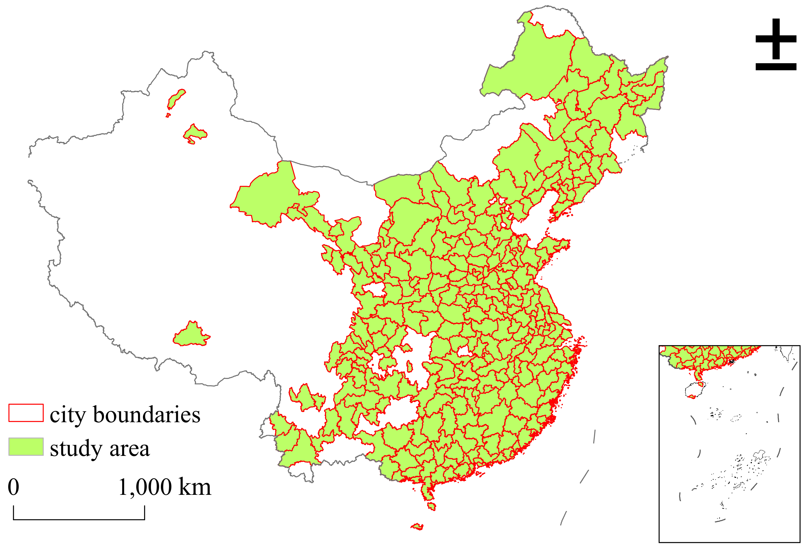
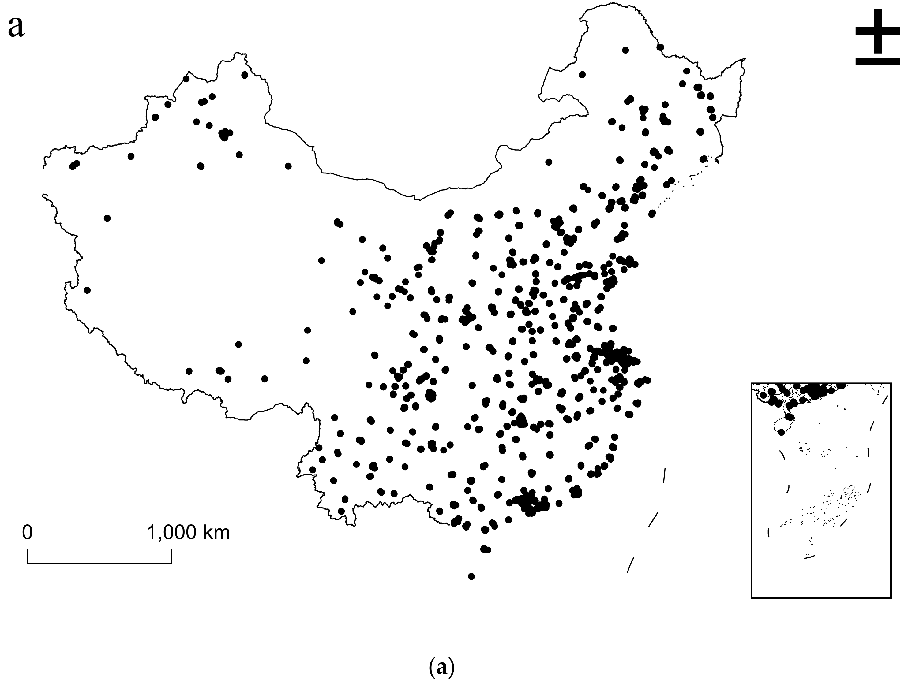
2.1. The Study Area

Figure 1 shows that the study area consists of 289 cities throughout China, which basically covers all the important cities in China. These cities were chosen on the condition of whether PM_2.5 monitoring points existed in the city and the availability of PM_2.5 data.

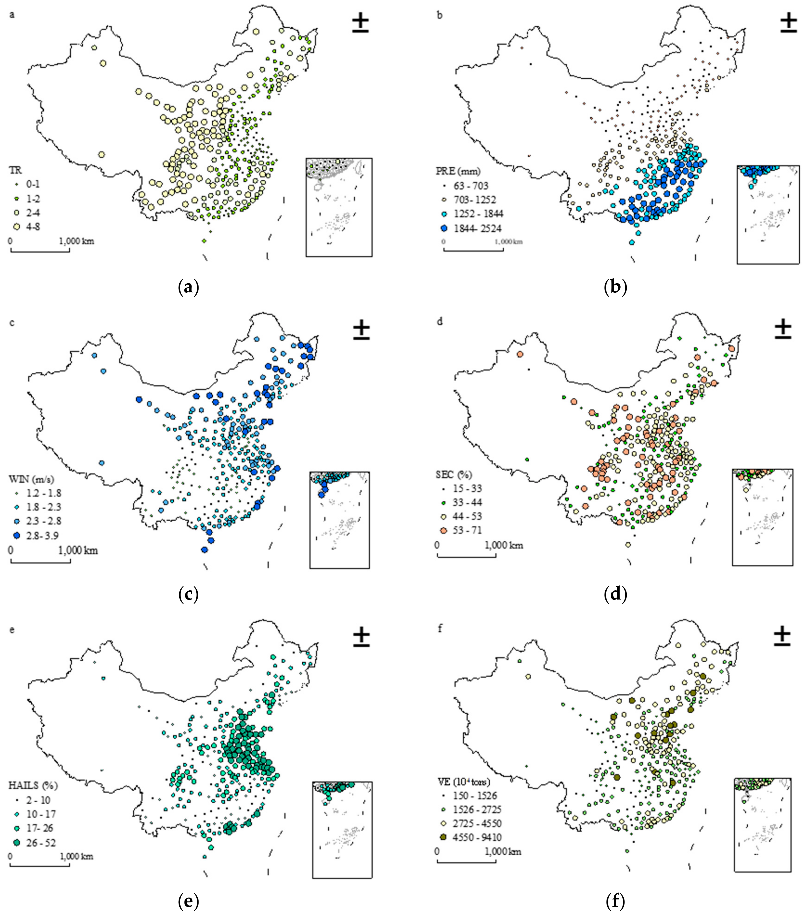
2.2. The Selected Explanatory Variables and Data Sources

This study explores the impacts of natural environmental conditions and socio-economic factors related to PM_2.5 pollution. In this section, the details of each explanatory variable are displayed (

Table 1. The selected natural environmental conditions and socio-economic factors related to particulate matter (PM_2.5) concentrations.

Variables	Abbreviation	Meaning
Terrain relief	TR	Relief degree of topography
Precipitation (mm)	PRE	Sum of daily precipitation in the year 2015
Wind speed (m/s)	WIN	Mean of daily average temperature
Human activity intensity of land surface (%)	HAILS	The extent of the impact of human activities on land surface
The secondary industry’s proportion (%)	SEC	The proportion of the secondary industry in the total social output value
The total particulate matter emissions of motor vehicles (104 tons)	VE	Total particulate matter emissions from motor vehicle exhaust

). Specifically, we selected precipitation (PRE, mm), terrain relief (TR) and wind speed (WIN, m/s) as the natural environmental conditions; while human activity intensity of land surface (HAILS, %), the secondary industry’s proportion (SEC, %), and the total particulate matter emissions of motor vehicles (VE, 10⁴ tons) were chosen as the socio-economic factors.

The PM_2.5 pollution data in 2015 comes from the National Urban Air Quality Online Monitoring Platform [43], which contains data from 1497 air pollution observation stations (Figure 2a). The PM_2.5 data was carried out in accordance with the standards stipulated by the rules of Ministry of National Ecological Environment Protection of China strictly [44]. In order to be consistent with the standard terminology of GB3095-2012 [45], the daily average in this paper represented the arithmetic average of the average concentration in 24 hours of a natural day, the monthly average represented the arithmetic average of the average concentration in one calendar month, and the annual average represented the arithmetic average of the average concentration in one calendar year. The daily average data was calculated based on the hourly monitoring data of each station, and then based on the daily average data, the monthly data was measured. Finally, the annual average PM_2.5 concentrations of 1497 stations were calculated according to the monthly average, and then these values were interpolated in space to obtain the annual average PM_2.5 concentrations of the selected cities. The meteorological data in 2015 came from the Resource and Environment Data Cloud Platform of the Institute of Geographic Sciences and Resources, Chinese Academy of Sciences (http://www.resdc.cn), which covered the data of all 2421 meteorological monitoring stations in China (Figure 2b). A spatial interpolation method (Inverse Distance Weighted (IDW)) was used to generate a national continuous surface for the meteorological data (including annual precipitation and annual average wind speed), and then the spatial statistical method was used to process the data to obtain the meteorological data of the 289 selected cities. The SEC data and the VE data in the 289 selected cities in 2015 were all from the statistical yearbook provided by the China Economic and Social Big Data Research Platform (http://data.cnki.net/). The HAILS data was calculated based on the algorithm proposed by Xu et al. [46], and the original data came from the China Statistical Yearbook for County Areas (2015) (http://data.cnki.net/). The TR data was calculated from the Digital Elevation Model (DEM), which came from the Cold and Arid Science Data Center (http://westdc.westgis.ac.cn).

2.3. Methods

This article first used Moran’s I to detect the spatial autocorrelation of PM_2.5 pollution in the 289 selected cities [47,48,49], and subsequently used regression analysis methods to detect the relationship between PM_2.5 pollution and the selected explanatory variables.

2.3.1. Spatial Autocorrelation Analysis Based on Moran’s I

In this paper, we used OpenGeoDa 1.12.1 software (Center for Spatial Data Science, University of Chicago, Chicago, Illinois https://www.uchicago.edu/research/center/center_for_spatial_data_science/) to achieve the spatial autocorrelation analysis. OpenGeoDa is a very practical tool for spatial statistical analysis, which is often used in spatial autoregressive analysis [50].

The global Moran’s I can be expressed by the following formula [51]:

$$I=\frac{n{\sum }_i{\sum }_{j\ne i}{w}_{ij}\left(y_i-\overline{y}\right)}{\left({\sum }_i{\sum }_{j\ne i}{w}_{ij}\right){\sum }_i{\left(y_i-\overline{y}\right)}^2}$$

(1)

where $w_{ij}$ represents the spatial weight matrix W, which corresponds to the geographic area ($i$, j), and $y_i$ and $y_j$ represent the observed values of $i$ and j, respectively. The Moran’s I value varies by [−1,1]. Positive values for Moran’s I denote positive spatial autocorrelation; conversely, negative values show the negative; and 0 indicates no correlation. The absolute values of Moran’s I are positively related to the spatial correlation of the selected variables.

Local autocorrelation analysis is usually used to identify hotspot areas by reflecting the correlation and similarity among adjacent units, which represents the state of PM_2.5 pollution gathering at spatial scale in this study. It could be expressed as [51]:

$$I=\frac{\left(x_i-\overline{x}\right)}{{\sum }_i{\left(x_i-\overline{x}\right)}^2}{\displaystyle \sum }_j{w}_{ij}\left(x_i-\overline{x}\right)$$

(2)

where $w_{ij}$ represents the spatial weight matrix W, which corresponds to the geographic area ($i$, j), and $y_i$ and $y_j$ represent the observed value of $i$ and j, respectively. In this paper, a Local Indicators of Spatial Association (LISA) agglomeration plot was used for analysis, which indicated the local spatial association of PM_2.5 pollution over space. There are four local spatial aggregation patterns on LISA agglomeration plot, namely the high–high type, the low–low type, the high–low type, and the low–high type. The high–high-type agglomeration and the low–low type agglomeration correspond to the positive spatial correlation in the global correlation index, while the low–high and high–low agglomeration correspond to the negative spatial correlation in the global correlation index.

2.3.2. Global Regression Model

The OLS model assumes that the variables are spatially stationary and it is usually utilized to quantitatively estimate the effects on a dependent variable, which is PM_2.5 concentration in this paper, caused by independent variables; however, if spatial correlation is ignored, it may lead to biased estimates. In order to solve this problem, the SLM and SEM were added in this paper. The SLM uses a lag variable to interpret the spatial autocorrelation, while SEM supplements the spatial correlation between different covariates that may be ignored through adopting error terms [52].

The OLS model could be displayed as:

$$\mathrm{y}={\beta }_0+{\displaystyle \sum }_{j=1}^p{\beta }_j{x}_j+\epsilon$$

(3)

where $\mathrm{y}$ means the PM_2.5 concentrations in sample cities, ${\beta }_0$ stands for the intercept, ${\beta }_j$ means the parameter estimate result for the selected explanatory variables $x_j$ ($j=1, \dots , p$), $p$ means the number of selected explanatory variables, and $\epsilon$ stands for the error vector, which follows a normal distribution.

A variable can be related to the neighbors occasionally. So, based on the hypothesis that the dependent variables will change with the variation of the neighbors, the SLM is proposed. The SLM could be expressed as:

$$\mathrm{y}={\beta }_0+\delta {\displaystyle \sum }_{j=1}^p{W}_{j}y+{\displaystyle \sum }_{j=1}^p{\beta }_j{x}_j+\epsilon$$

(4)

where $\delta$ stands for the parameter estimate result of a spatial lag term, indicating the variation of spatial autocorrelation of $\mathrm{y}$ (when $\delta$ gets larger, the spatial autocorrelation of $\mathrm{y}$ gets higher); $W_j$ is a matrix of spatial weights of the dependent variable $\mathrm{y}$. In this paper, we utilized the IDW as the method of spatial lag term weight.

When the OLS is applied to spatially related variables, the spatial correlation of the error terms is usually unavoidable, which contradicts the basic hypothesis of the OLS model. To solve the problem, the SEM resolves the impacts by the error term. The SEM model could be explained as:

$$\mathrm{y}={\beta }_0+{\displaystyle \sum }_{j=1}^p{\beta }_j{x}_j+\mu {\displaystyle \sum }_{j=1}^p{W}_j^{\prime }\epsilon$$

(5)

where $\mu$ is the parameter estimate result of the error term, denoting the autocorrelation of the model’s error term (when $\mu$ gets larger, the spatial autocorrelation of dependent variable gets higher); $W_j^{\prime }$ is a matrix of spatial weights of the error term $\epsilon$. To be consistent with the SLM, we utilized the IDW as the method of spatial error term weight.

In addition, the coefficient of determination and the Akaike information criterion (abbreviated as R² and AIC, respectively) were utilized in this paper to evaluate the simulation results of the global regression models. These two indices are often used to measure the fitting degree of various models; specifically, lower values of R² values and higher values of AIC represents not ideal models [53,54].

2.3.3. Local Regression Model

Although global regression models can describe the significance of statistical relationships between dependent and independent variables, it always results in problems by using global regression models because of the assumption that the variables have homogeneity. In other words, global regression models could not detect the potentially important local changes of the data [55]. To make up for this deficiency, the GWR model was added in this paper. The GWR model incorporates spatial location attributes of data into regression parameters. The GWR model uses local weighted ordinary least squares to estimate point parameters, whose weight is the distance function from the position of the regression point to the locations of other sample points. [56]. The GWR model could be explained as:

$$\ln y_j={\beta }_{j0}+{\displaystyle \sum }_{j=1}^n{\beta }_{jn}{x}_{jn}+{\epsilon }_j$$

(6)

where $j=1,\dots , 289$ represents spatial locations of the selected cities; $y_j$ represents the PM_2.5 concentration of the $j$ province (the dependent variable); six independent variables $x_{jn} \left(n=1,\dots ,6\right)$, including TR, PRE, WIN, SEC, HAILS, and VE; ${\beta }_{jn}$ are the local regression parameters; and ${\epsilon }_j$ means the random error, by which each sample city in this paper has a set of corresponding parameters to detect the correlations between PM_2.5 pollution and related factors.

3. Results

3.1. Spatial Variation Characteristics of PM_2.5 Pollution and the Selected Explanatory Variables

Figure 3 reflects the spatial variation of PM_2.5 pollution in the selected 289 areas. In 2015, the annual average PM_2.5 concentration in the 289 sample cities was 56.6$\mathsf{\mu }\mathrm{g}/{\mathrm{m}}^3$, and the five cities with the highest annual average concentration were Baoding, Xingtai, Hengshui, Dezhou, and Liaocheng. The annual average of the first four cities was greater than 100 $\mathsf{\mu }\mathrm{g}/{\mathrm{m}}^3$. According to (GB 3095-2012 Revision) the latest edition of the Ambient Air Quality Standard of the Ministry of National Environmental Protection of the People’s Republic of China [45], the ambient air function is divided into two categories (

Table 2. PM_2.5 concentration standards of China ($\mathsf{\mu }\mathrm{g}/{\mathrm{m}}^3$).

Concentration Limits	Annual Mean	24-h Average
Level 1th	15	35
Level 2th	35	75

). The level 1th standard is applicable to the special areas such as nature reserves and scenic sites, where the annual average and daily limits of PM_2.5 concentration are 15 $\mathsf{\mu }\mathrm{g}/{\mathrm{m}}^3$ and 35 $\mathsf{\mu }\mathrm{g}/{\mathrm{m}}^3$, respectively. The level 2th standard is applicable to residential, cultural, commercial, industrial, and rural areas, where the annual and daily limits are 35 $\mathsf{\mu }\mathrm{g}/{\mathrm{m}}^3$ and 75 $\mathsf{\mu }\mathrm{g}/{\mathrm{m}}^3$, respectively. In 2015, the annual average PM_2.5 concentrations of only 51 cities were lower than 35 $\mathsf{\mu }\mathrm{g}/{\mathrm{m}}^3$; the annual average PM_2.5 concentrations of 209 cities were between 35 and 75 $\mathsf{\mu }\mathrm{g}/{\mathrm{m}}^3$; the annual average PM_2.5 concentrations of 29 cities were higher than 75 $\mathsf{\mu }\mathrm{g}/{\mathrm{m}}^3$.

Figure 4a reflects the spatial variation of TR in the study area. Overall, the eastern coastal cities have less terrain relief than the northwestern inland cities. Among them, the city with the lowest terrain relief was Yancheng, followed by Panjin and Nantong, and the city with the largest terrain relief was Weinan. Figure 4b reflects the spatial distribution of PRE in the study area. Huangshan (2524 mm) had the most abundant precipitation, while the most arid city was Jiayuguan (63 mm). Figure 4d reflects the development of secondary industry in each selected city. Panzhihua’s SEC accounted for 71.45%, the highest proportion of all sample cities, and Heihe (15.17%) was the city with the lowest SEC. Figure 4e reflects the spatial distribution of HAILS of the selected cities. The city with the strongest HAILS was Shanghai (51.25%), followed by Beijing (49.47%), and the city with the lowest HAILS was Lhasa (5.7%). Figure 4f reflects the spatial distribution of VE in selected cities. Handan (94.1 million tons) had the highest emissions, followed by Chongqing (72.7 million tons), while Beihai (2.6 million tons) had the lowest emissions.

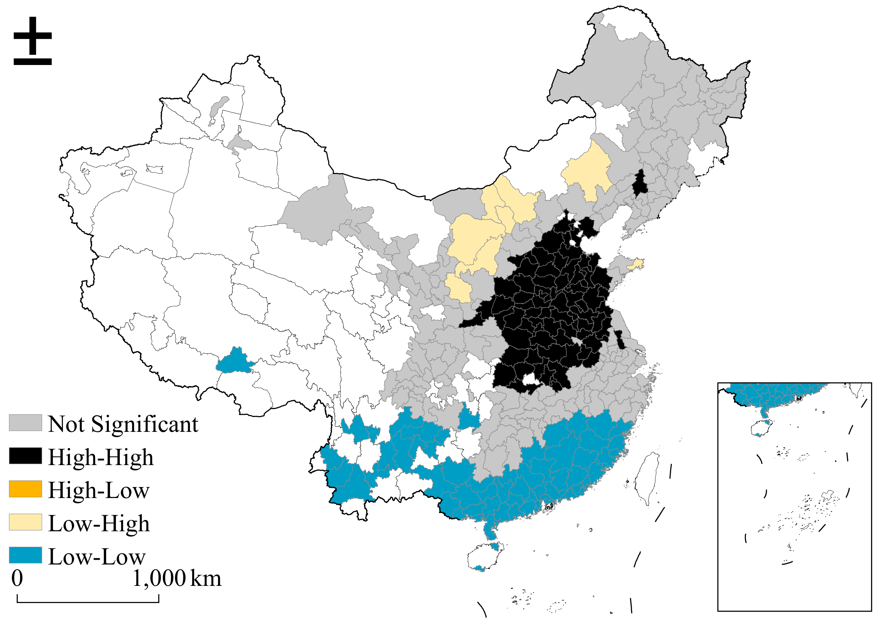
3.2. Spatial Agglomeration of PM_2.5 Pollution Based on Moran’s I

The spatial autocorrelation test of the agglomeration characteristics of PM_2.5 pollution in selected cities was carried out using OpenGeoDa. By constructing the spatial distance weight matrix, the Moran’s I value of PM_2.5 pollution in selected cities is 0.8406 (p < 0.01), which reflects significant spatial autocorrelation of PM_2.5 pollution in selected cities in 2015.

Figure 5 reveals that agglomeration characteristics of PM_2.5 pollution in China were particularly significant in the Beijing–Tianjin–Hebei region. The spatial distribution of PM_2.5 concentrations in Chinese cities in 2015 had evident spatial dependence and spatial spillover effects.

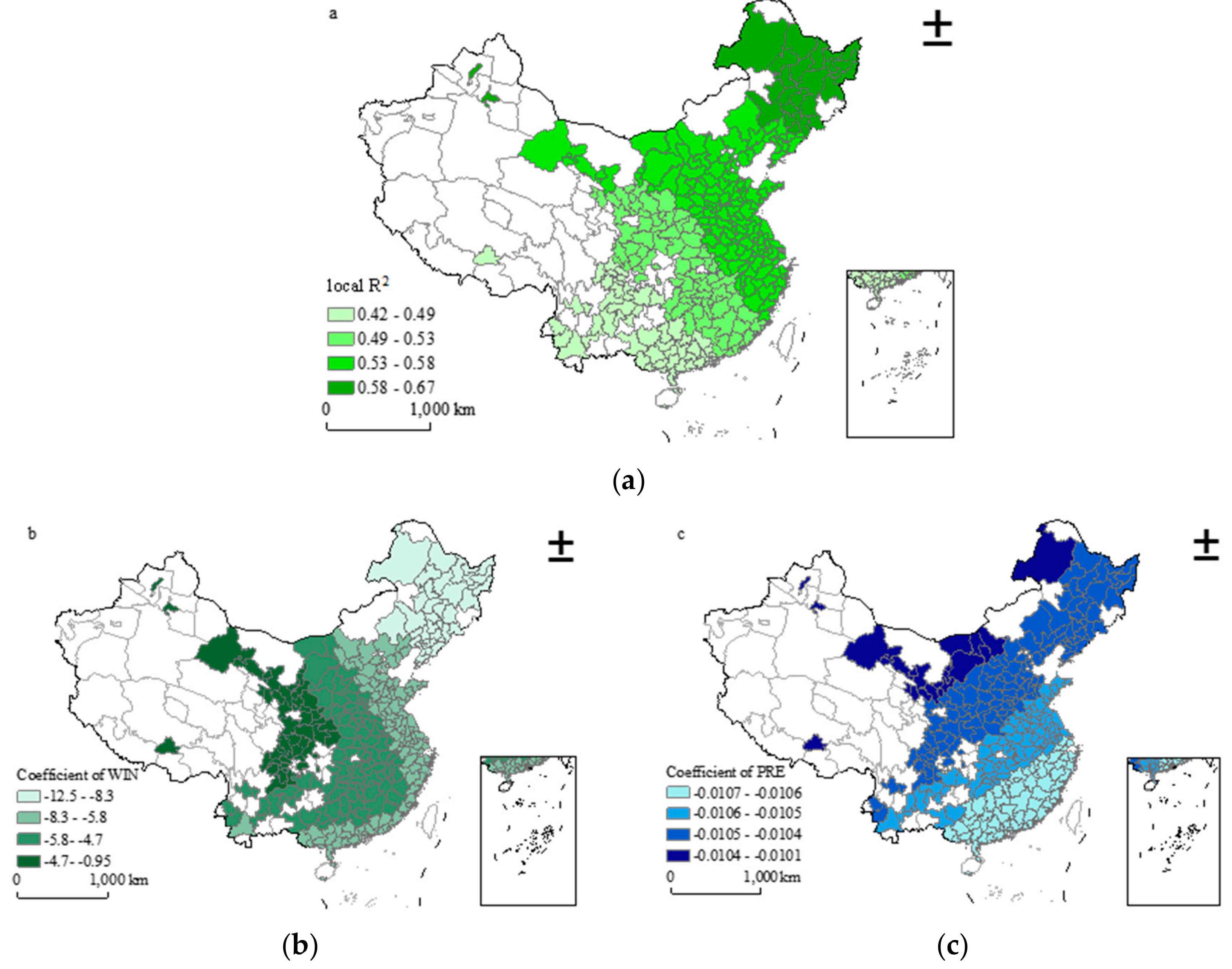
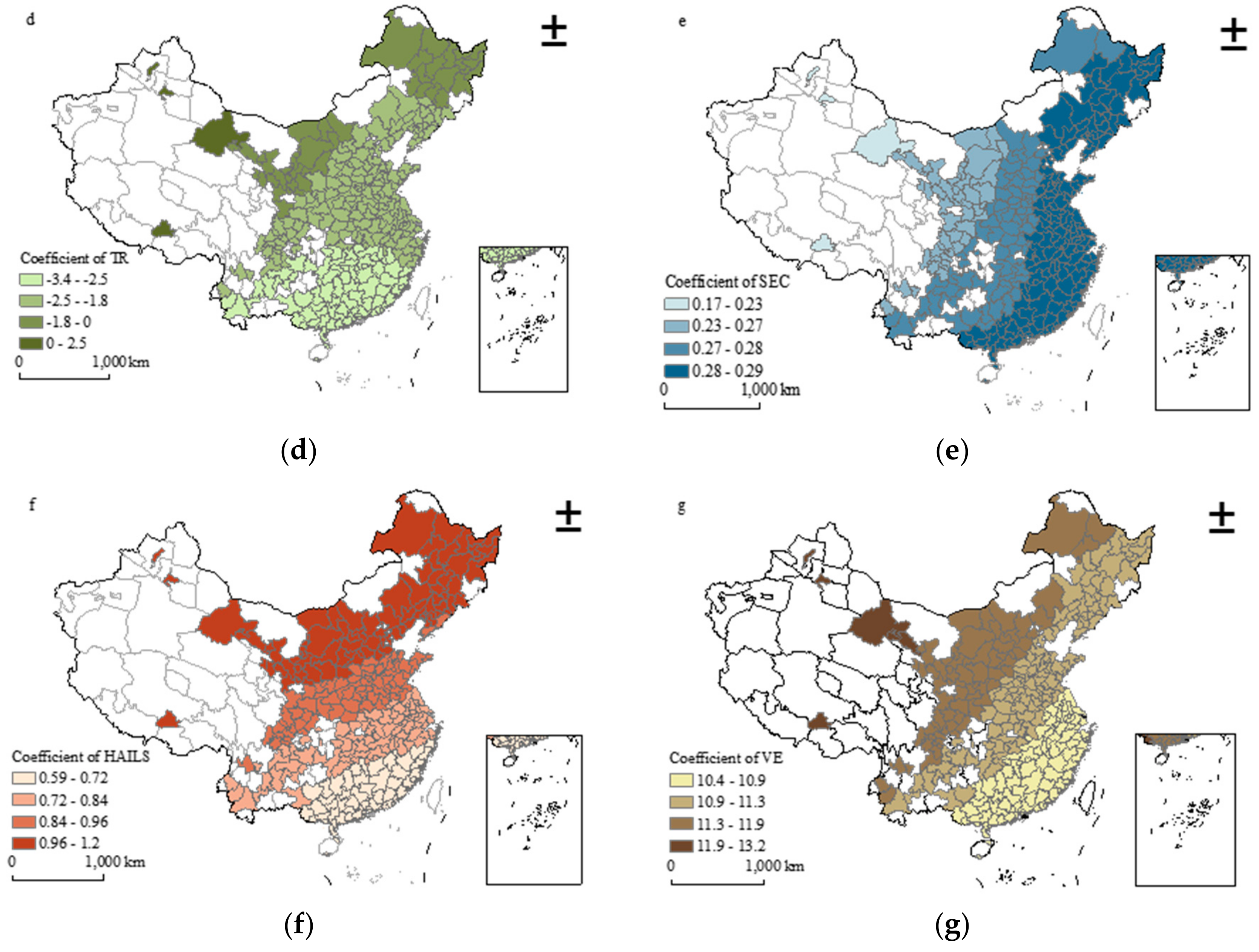
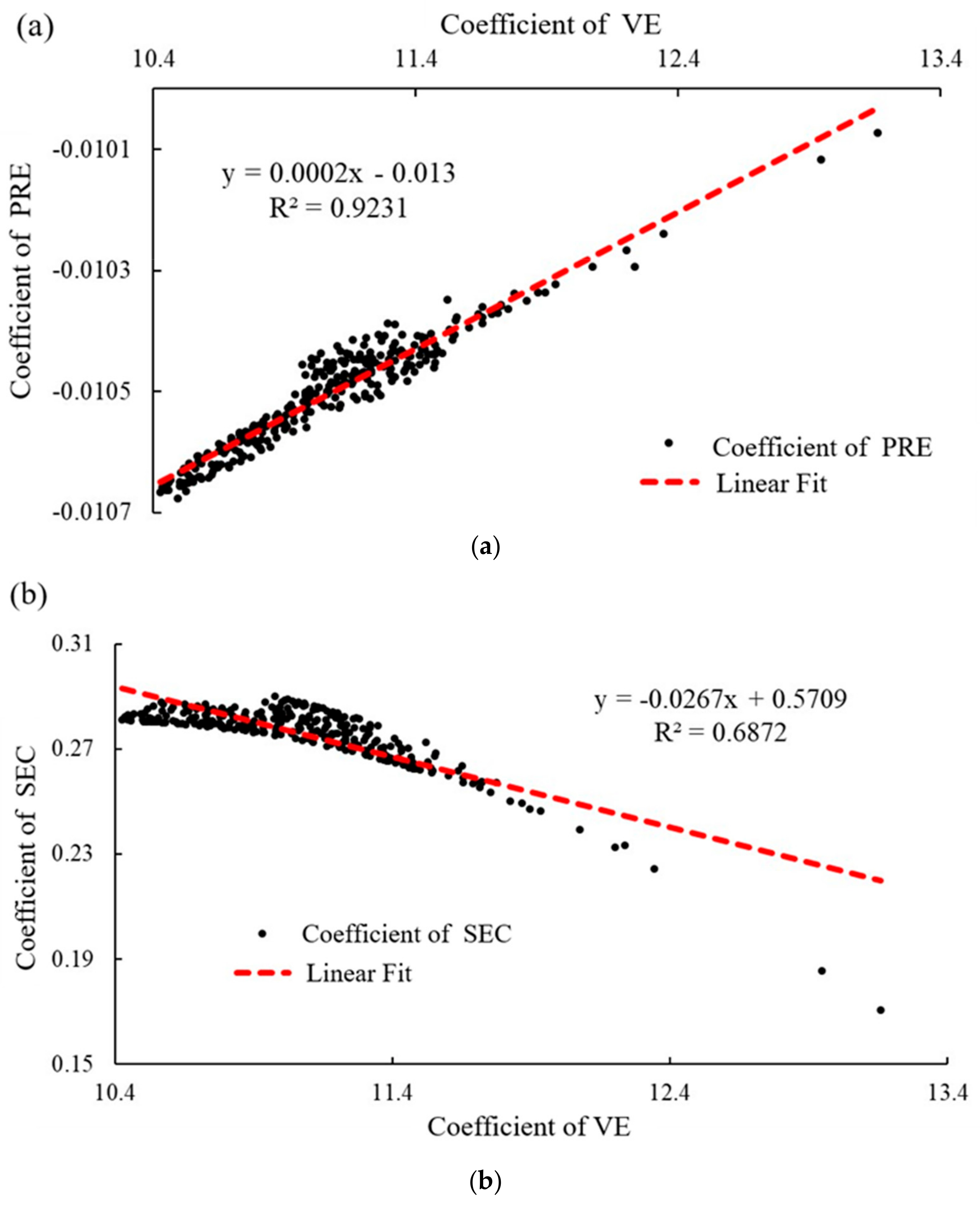
3.3. Analysis of the Relationship Between PM_2.5 Pollution and the Explanatory Variables Based on Regression Models

Table 3. The correlation analysis between PM_2.5 concentrations and the selected explanatory variables based on global regression models (N = 289).

Variables	OLS Results	SLM Results	SEM Results
TR	−1.51	−0.81	−0.41
WIN (m/s)	−5.82 *	−1.5 **	−4.14 *
SEC (%)	0.25 **	0.07 ***	0.06 ***
VE (104 tons)	8.26 *	5.52 **	3.85 **
PRE (mm)	−0.017 **	−0.031 ***	−0.04 ***
HAILS (%)	0.67 *	0.32 *	0.27 **
Lag parameter	−	0.581 **	−
Lambda (spatial error parameter)	−	−	0.592 **
R-squared	0.513	0.612	0.631
AIC	2216.83	1918.81	1808.87

Note: *, **, and *** means that the significance is at the 5% level, 1% level, and 0.1% level, respectively.

lists the estimated results of the relationship between PM_2.5 pollution and the explanatory variables based on three global regression models. The values of R² of the SLM model and the SEM model were 0.612 and 0.631, respectively, which were significantly higher than the result of the OLS model (0.513), indicating that the interpretation effect by using the SLM model and the SEM model was obviously better than using the OLS model. Furthermore, the SEM resulted in lesser AIC (1808.87) values than that of the SLM (1918.81), which meant the results of the SEM was better than the SLM. Taking the above into consideration, we chose the results of the SEM as the global regression analysis results.

From Table 3, we can see that no evident correlation existed between TR and PM_2.5 concentrations; while WIN and VE maintained the most significant correlation with PM_2.5 concentrations. WIN was obviously negatively correlated with PM_2.5 concentrations, namely, every 1 m/s increase in wind speed could decrease PM_2.5 concentrations by 4.14 $\mathsf{\mu }\mathrm{g}/{\mathrm{m}}^3$. VE was specially positively correlated with PM_2.5 concentrations, which meant every 10,000 tons increase in VE could increase PM_2.5 concentration by 3.85 $\mathsf{\mu }\mathrm{g}/{\mathrm{m}}^3$. HAILS was positively correlated with PM_2.5 concentrations, denoting that every 1% rise in HAILS contributed to 0.27 $\mathsf{\mu }\mathrm{g}/{\mathrm{m}}^3$ increase in PM_2.5 concentration. The correlation coefficient of PRE was −0.04, indicating a weak negative correlation between PRE and PM_2.5 concentration. For every 1 mm increase in precipitation, PM_2.5 concentration would reduce by 0.04 $\mathsf{\mu }\mathrm{g}/{\mathrm{m}}^3$. The coefficient of SEC was 0.06, indicating a weak positive correlation between SEC and PM_2.5 concentrations. For every 1% rise in SEC, the PM_2.5 concentration would increase by 0.06 $\mathsf{\mu }\mathrm{g}/{\mathrm{m}}^3$. In addition, the value of Lambda denoted an evident relationship with the PM_2.5 concentration, meaning that undiscovered spatial autocorrelation existed in the data.

The GWR model was then introduced to further analyze the local characteristics of the relation between PM_2.5 pollution and the selected explanatory variables. The R² of the GWR model was 0.734, which meant that 73.4% of the variability of the PM_2.5 pollution could be explained by the GWR model. Furthermore, the value of R² was higher than the estimation results obtained by the global models, which indicated the interpretation effectiveness of the GWR model behaved superior to the results of the OLS model, the SLM, and the SEM.

Figure 6a reveals the spatial distribution difference of local R², which increased from southwest to northeast (varying from 0.42 to 0.67). The variety of local R² suggested when comprehensively considering the effects of all the six explanatory variables, the spatially correlated relationship was more conclusively in northeastern cites than in other regions. At 0.67, Jiamusi had the largest local R² value, while Simao got the lowest local R² value of 0.42.

Figure 6b reveals the spatial correlation between WIN and PM_2.5 pollution. The PM_2.5 concentration of Dalian had the strongest negative correlation with wind speed, and when the wind speed in Dalian increased by 1 m/s, the PM_2.5 concentration could be reduced by 12.5 $\mathsf{\mu }\mathrm{g}/{\mathrm{m}}^3$. Overall, there existed an evident negative relationship between WIN and PM_2.5 concentrations. The higher the wind speed, the lower the PM_2.5 concentration, and the faster the PM_2.5 pollution would be eliminated. In addition, it could be seen that from the eastern coast areas to the northwest inland areas, the effect of WIN on PM_2.5 pollution gradually weakened.

Figure 6c reveals the spatial correlation between PRE and PM_2.5 pollution. Guangzhou’s PM_2.5 concentration showed the strongest negative correlation with PRE (−0.0107), which meant when precipitation in Guangzhou increased by 1 mm, the PM_2.5 concentration could be reduced by 0.0107 $\mathsf{\mu }\mathrm{g}/{\mathrm{m}}^3$. Similar to WIN, there was also a negative correlation between PRE and PM_2.5 concentrations, but the effect of PRE on PM_2.5 concentrations was significantly weaker. In addition, PRE in southeastern coastal areas was more beneficial to reducing PM_2.5 pollution than in the northwestern hinterland areas.

Figure 6d reveals the spatial correlation between TR and PM_2.5 pollution. Unlike the results of WIN and PRE, the spatial correlation between TR and PM_2.5 pollution was not spatially consistent. There existed a positive correlation between TR and PM_2.5 pollution in cities such as Urumqi (2.5) and Jiuquan (2.3) in the northwestern hinterland areas, indicating that the increase in TR in these areas would increase PM_2.5 concentrations. However, except for the few cities in the northwestern inland areas, we found negative correlations between TR and PM_2.5 concentrations in other areas. The PM_2.5 concentration in Haikou showed the strongest negative correlation (−3.4) with TR, which meant that when the TR of Haikou increased by 1, the PM_2.5 concentration could be reduced by 3.4 $\mathsf{\mu }\mathrm{g}/{\mathrm{m}}^3$.

Figure 6e reveals the spatial correlation between SEC and PM_2.5 pollution in the 289 selected cities. SEC showed a positively correlation with PM_2.5 pollution. Xiamen’s PM_2.5 concentration had the strongest positive correlation with SEC (0.29), indicating that for every 1% rise in SEC in Xiamen, the PM_2.5 concentration would increase by 0.29 $\mathsf{\mu }\mathrm{g}/{\mathrm{m}}^3$.

Figure 6f reveals the spatial correlation between HAILS and PM_2.5 pollution. From south to north, the relationship between the two was gradually enhanced (varying from 0.59 to 1.2). The PM_2.5 concentration of Qiqihar had the strongest positive correlation with HAILS (1.2), indicating that the PM_2.5 concentration of Qiqihar would increase by 1.2 $\mathsf{\mu }\mathrm{g}/{\mathrm{m}}^3$ for every 1% increase in HAILS.

Figure 6g reveals a significant positive correlation between VE and PM_2.5 pollution. Urumqi’s PM_2.5 concentration was the strongest positive correlation with VE (13.2), indicating that PM_2.5 concentration would increase by 13.2 $\mathsf{\mu }\mathrm{g}/{\mathrm{m}}^3$ for every 10,000 tons increase in VE in Urumqi. In addition, from the perspective of spatial variation trends, motor vehicle exhaust emissions in the northwest inland areas were more likely to cause PM_2.5 pollution than in the southeastern coastal areas.

4. Discussion

This study revealed that on the whole, PRE showed a negative relation to PM_2.5 pollution, while VE and SEC maintained a positive relation to PM_2.5 pollution—a finding that is generally consistent with that of related previous studies by Guo et al (2017) [57] and Wong et al (2019) [58].

Figure 7a shows that the value of the coefficient of PRE was reduced when the value of the coefficient of VE increased, which meant that in areas where VE was the critical factor leading to PM_2.5 pollution, the mitigation effect of PRE on PM_2.5 concentrations was weak. Similarly, Figure 7b suggests that in areas where VE was the critical factor leading to PM_2.5 pollution, the mitigation effect of SEC on PM_2.5 concentrations was weak. Therefore, in areas where the coefficient of VE was high, the impact of other natural environmental conditions and socio-economic factors such as PRE and SEC on PM_2.5 pollution would become weak.

In brief, VE had the most significant effect on PM_2.5 concentrations among these related factors, which means controlling motor vehicle pollutant emissions is an important measure to reduce PM_2.5 pollution in China. As the largest developing country all over the world, China is suffering seriously from the damage caused by PM_2.5 pollution, which was linked with 0.964 million to 1.258 million deaths each year [59]. The sustainable development policy has been actively promoted by the Chinese government in recent years, which is plagued by severe PM_2.5 pollution. To achieve the goal of sustainable development, China needs to actively promote motor vehicles using clean energy.

5. Conclusions

Since 2013, the Chinese government has been vigorously advocating for PM_2.5 pollution control, but the results have not been significant. This paper analyzed the natural environmental conditions and the socio-economic factors related to the spatial variation of PM_2.5 concentrations based on a panel study of 289 cities. The conclusions drawn in this study are as follows.

First, the PM_2.5 concentrations in most cities in China exceeded their limits in 2015. The PM_2.5 pollution is not limited to a certain city or a certain area but is a nationwide problem. The average PM_2.5 concentration of the 289 selected cities in 2015 was 56.6 $\mathsf{\mu }\mathrm{g}/{\mathrm{m}}^3$, and there were only 51 cities with PM_2.5 concentrations up to standard, accounting for 17.6% of the total sample cities. The spatial agglomeration characteristics of PM_2.5 pollution in China were particularly significant in the Beijing–Tianjin–Hebei region.

Second, the global regression models’ results confirmed the significantly different spatial correlations between PM_2.5 pollution and the six selected explanatory variables. Specifically, there existed no significant correlation between TR and the PM_2.5 concentration; every 1 m/s increase in WIN could decrease the PM_2.5 concentration by 4.14 $\mathsf{\mu }\mathrm{g}/{\mathrm{m}}^3$; every 10,000 tons increase in VE could increase the PM_2.5 concentration by 3.85 $\mathsf{\mu }\mathrm{g}/{\mathrm{m}}^3$; the PM_2.5 concentration increased by 0.27 $\mathsf{\mu }\mathrm{g}/{\mathrm{m}}^3$ with 1% increase in HAILS; every 1 mm increase in PRE would lead to a 0.04 $\mathsf{\mu }\mathrm{g}/{\mathrm{m}}^3$ reduction of the PM_2.5 concentration; and every 1% rise in SEC could result in a 0.06 $\mathsf{\mu }\mathrm{g}/{\mathrm{m}}^3$ rise in the PM_2.5 concentration.

Third, the simulation results of GWR l are better than those of the OLS model, the SLM, and the SEM model in explaining the local correlations between PM_2.5 concentrations and related factors. Overall, the effects of different explanatory variables on PM_2.5 concentrations varied greatly with geographical locations. When considering the comprehensive effects of all the six explanatory variables, the spatially correlated relationship was more conclusive in the northeastern cities than in other regions. VE had the greatest impact on PM_2.5 concentrations, and the impact intensity gradually increased from eastern coastal areas to the northwest inland areas. Among the three selected natural environmental conditions, WIN had the greatest impact on PM_2.5 concentrations, and the impact weakened from eastern coastal areas to northwest inland areas.

Fourth, the application of the GWR model improved the regression accuracy to a large extent by displaying fit characteristics compared with the results of the three global regression models.

What needs to be stated here is that the purpose of this paper is to detect the influence of related factors on spatial variations, rather than the temporal variations of PM_2.5 pollution. Therefore, the results can only be used to show the spatial variations of PM_2.5 pollution and cannot explain the temporal differences. This paper, which explored how the natural environmental conditions and socio-economic factors influence PM_2.5 pollution utilizing various regression models, provides a comprehensive perspective for further research.

References

1. Spengler, J.D.; Fay, M.E.; Ferris, B.G.; Dockery, D.W.; Ware, J.H.; Pope, C.A.; Xu, X.; Speizer, F.E. An Association between Air Pollution and Mortality in Six U.S. Cities. New Engl. J. Med. 1993, 329, 1753–1759. [Google Scholar] [Green Version]
2. Mayer, H. Air pollution in cities. Atmospheric Environ. 1999, 33, 4029–4037. [Google Scholar] [CrossRef]
3. Lelieveld, J.; Evans, J.S.; Fnais, M.; Giannadaki, D.; Pozzer, A. The contribution of outdoor air pollution sources to premature mortality on a global scale. Nature 2015, 525, 367–371. [Google Scholar] [CrossRef] [PubMed]
4. Ning, G.; Wang, S.; Ma, M.; Ni, C.; Shang, Z.; Wang, J.; Li, J. Characteristics of air pollution in different zones of Sichuan Basin, China. Sci. Total. Environ. 2018, 612, 975–984. [Google Scholar] [CrossRef] [PubMed]
5. Peters, I.M.; Karthik, S.; Liu, H.; Buonassisi, T.; Nobre, A. Urban haze and photovoltaics. Energy Environ. Sci. 2018, 11, 3043–3054. [Google Scholar] [CrossRef] [Green Version]
6. Silver, B.; Reddington, C.L.; Arnold, S.R.; Spracklen, D.V.; Reddington, C.; Arnold, S. Substantial changes in air pollution across China during 2015–2017. Environ. Res. Lett. 2018, 13, 114012. [Google Scholar] [CrossRef]
7. Zhao, S.; Liu, S.; Hou, X.; Beazley, R.; Sun, Y. Identifying the contributions of multiple driving forces to PM10–2.5 pollution in urban areas in China. Sci. Total. Environ. 2019, 663, 361–368. [Google Scholar] [CrossRef]
8. Polezer, G.; Tadano, Y.S.; Siqueira, H.V.; Godoi, A.F.; Yamamoto, C.I.; De Andre, P.A.; Pauliquevis, T.; Andrade, M.D.F.; Oliveira, A.; Saldiva, P.H.; et al. Assessing the impact of PM2.5 on respiratory disease using artificial neural networks. Environ. Pollut. 2018, 235, 394–403. [Google Scholar] [CrossRef]
9. Suleiman, A.; Tight, M.R.; Quinn, A.D. Applying machine learning methods in managing urban concentrations of traffic-related particulate matter (PM10 and PM2.5). Atmos. Pollut. 2018, 10, 134–144. [Google Scholar] [CrossRef]
10. Williams, A.M.; Phaneuf, D.J.; Barrett, M.A.; Su, J.G. Short-term impact of PM2.5 on contemporaneous asthma medication use: behavior and the value of pollution reductions. P. Natl. Acad. Sci. USA. 2019, 116, 5246–5253. [Google Scholar] [CrossRef]
11. Bautista, L. Cardiovascular impact of PM2.5 from the emissions of coal-fired power plants in Spain during 2014 Impacto cardiovascular del PM2.5 procedente de las emisiones de las centrales térmicas de carbón en España durante el año 2014. Med. Clin-Barcelona. 2019, 153, 100–105. [Google Scholar]
12. Schmitt, L.H.M. QALY gain and health care resource impacts of air pollution control: A Markov modelling approach. Environ. Sci. Policy 2016, 63, 35–43. [Google Scholar] [CrossRef] [Green Version]
13. Cakmak, S.; Hebbern, C.; Cakmak, J.D.; Vanos, J. The modifying effect of socioeconomic status on the relationship between traffic, air pollution and respiratory health in elementary schoolchildren. J. Environ. Manag. 2016, 177, 1–8. [Google Scholar] [CrossRef] [PubMed] [Green Version]
14. Dabass, A.; Talbott, E.O.; Bilonick, R.A.; Rager, J.R.; Venkat, A.; Marsh, G.M.; Duan, C.; Xue, T. Using spatio-temporal modeling for exposure assessment in an investigation of fine particulate air pollution and cardiovascular mortality. Environ. Res. 2016, 151, 564–572. [Google Scholar] [CrossRef] [PubMed] [Green Version]
15. Zhu, G.; Hu, W.; Liu, Y.; Cao, J.; Ma, Z.; Deng, Y.; Sabel, C.E.; Wang, H. Health burdens of ambient PM2.5 pollution across Chinese cities during 2006–2015. J. Environ. Manag. 2019, 243, 250–256. [Google Scholar] [CrossRef] [PubMed]
16. Dabass, A.; Talbott, E.; Rager, J.; Marsh, G.; Venkat, A.; Holguin, F.; Sharma, R. Systemic inflammatory makers associated with cardiovascular disease and acute and chronic exposure to fine particulate matter air pollution (PM2.5) among US NHANES adults with metabolic syndrome. Environ. Res. 2018, 161, 485–491. [Google Scholar] [CrossRef] [PubMed]
17. Lv, B. Characterizations of PM2.5 Pollution Pathways and Sources Analysis in Four Large Cities in China. Aerosol Air Qual. Res. 2015, 15, 1836–1843. [Google Scholar] [CrossRef]
18. Liao, T.; Wang, S.; Ai, J.; Gui, K.; Duan, B.; Zhao, Q.; Zhang, X.; Jiang, W.; Sun, Y. Heavy pollution episodes, transport pathways and potential sources of PM2.5 during the winter of 2013 in Chengdu (China). Sci. Total. Environ. 2017, 584, 1056–1065. [Google Scholar] [CrossRef]
19. Du, Y.; Sun, T.; Peng, J.; Fang, K.; Liu, Y.; Yang, Y.; Wang, Y. Direct and spillover effects of urbanization on PM2.5 concentrations in China’s top three urban agglomerations. J. Clean. Prod. 2018, 190, 72–83. [Google Scholar] [CrossRef]
20. Kuula, J.; Kuuluvainen, H.; Rönkkö, T.; Niemi, J.V.; Saukko, E.; Portin, H.; Aurela, M.; Saarikoski, S.; Rostedt, A.; Hillamo, R.; et al. Applicability of Optical and Diffusion Charging-Based Particulate Matter Sensors to Urban Air Quality Measurements. Aerosol Air Qual. Res. 2019, 19, 1024–1039. [Google Scholar] [CrossRef]
21. Xu, C.; Wu, S. Evaluating the Effects of Household Characteristics on Household Daily Traffic Emissions Based on Household Travel Survey Data. Sustainability 2019, 11, 1684. [Google Scholar] [CrossRef]
22. Ngo, N.S.; Asseko, S.V.J.; Ebanega, M.O.; Allo’O, S.M.A.; Hystad, P. The relationship among PM2.5, traffic emissions, and socioeconomic status: Evidence from Gabon using low-cost, portable air quality monitors. Transp. Res. Part D: Transp. Environ. 2019, 68, 2–9. [Google Scholar] [CrossRef]
23. Hao, Y.; Liu, Y.-M. The influential factors of urban PM2.5 concentrations in China: a spatial econometric analysis. J. Clean. Prod. 2016, 112, 1443–1453. [Google Scholar] [CrossRef]
24. Shen, G. Changes from traditional solid fuels to clean household energies – Opportunities in emission reduction of primary PM2.5 from residential cookstoves in China. Biomass Bioenerg. 2016, 86, 28–35. [Google Scholar] [CrossRef]
25. Lai, A.; Shan, M.; Deng, M.; Carter, E.; Yang, X.; Baumgartner, J.; Schauer, J. Differences in chemical composition of PM2.5 emissions from traditional versus advanced combustion (semi-gasifier) solid fuel stoves. Chemosphere 2019, 233, 852–861. [Google Scholar] [CrossRef] [PubMed]
26. Fenech, S.; Doherty, R.M.; Heaviside, C.; MacIntyre, H.L.; O’Connor, F.M.; Vardoulakis, S.; Neal, L.; Agnew, P. Meteorological drivers and mortality associated with O3 and PM2.5 air pollution episodes in the UK in 2006. Atmospheric Environ. 2019, 213, 699–710. [Google Scholar] [CrossRef]
27. Alvarez, H.A.O.; Myers, O.B.; Weigel, M.; Armijos, R.X. The value of using seasonality and meteorological variables to model intra-urban PM2.5 variation. Atmospheric Environ. 2018, 182, 1–8. [Google Scholar] [CrossRef] [PubMed] [Green Version]
28. Zalakeviciute, R.; Lopez-Villada, J.; Rybarczyk, Y. Contrasted Effects of Relative Humidity and Precipitation on Urban PM2.5 Pollution in High Elevation Urban Areas. Sustainability 2018, 10, 2064. [Google Scholar] [CrossRef]
29. Ryu, J.; Kim, J.J.; Byeon, H.; Go, T.; Lee, S.J. Removal of fine particulate matter (PM2.5) via atmospheric humidity caused by evapotranspiration. Environ. Pollut. 2019, 245, 253–259. [Google Scholar] [CrossRef]
30. De Hoogh, K.; Héritier, H.; Stafoggia, M.; Künzli, N.; Kloog, I. Modelling daily PM2.5 concentrations at high spatio-temporal resolution across Switzerland. Environ. Pollut. 2018, 233, 1147–1154. [Google Scholar] [CrossRef]
31. Rahman, A.; Luo, C.; Khan, M.; Ke, J.; Thilakanayaka, V.; Kumar, S. Influence of atmospheric PM2.5, PM10, O3, CO, NO2, SO2, and meteorological factors on the concentration of airborne pollen in Guangzhou. China. Atmos. Environ. 2019, 212, 290–304. [Google Scholar]
32. Miettinen, M.; Leskinen, A.; Abbaszade, G.; Orasche, J.; Sainio, M.; Mikkonen, S.; Koponen, H.; Rönkkö, T.; Ruusunen, J.; Kuuspalo, K.; et al. PM2.5 concentration and composition in the urban air of Nanjing, China: Effects of emission control measures applied during the 2014 Youth Olympic Games. Sci. Total. Environ. 2019, 652, 1–18. [Google Scholar] [CrossRef] [PubMed]
33. Jia, S.; Sarkar, S.; Zhang, Q.; Wang, X.; Wu, L.; Chen, W.; Huang, M.; Zhou, S.; Zhang, J.; Yuan, L.; et al. Characterization of diurnal variations of PM2.5 acidity using an open thermodynamic system: A case study of Guangzhou, China. Chemosphere 2018, 202, 677–685. [Google Scholar] [CrossRef] [PubMed]
34. Wang, Q.; Kwan, M.-P.; Zhou, K.; Fan, J.; Wang, Y.; Zhan, D. Impacts of residential energy consumption on the health burden of household air pollution: Evidence from 135 countries. Energy Policy 2019, 128, 284–295. [Google Scholar] [CrossRef]
35. Jia, R.; Khadka, A.; Kim, I. Traffic crash analysis with point-of-interest spatial clustering. Accid. Anal. Prev. 2018, 121, 223–230. [Google Scholar] [CrossRef]
36. Guo, S.; Lu, J. Jurisdictional air pollution regulation in China: A tragedy of the regulatory anti-commons. J. Clean. Prod. 2019, 212, 1054–1061. [Google Scholar] [CrossRef]
37. Oshan, T.; Wolf, L.J.; Fotheringham, A.S.; Kang, W.; Li, Z.; Yu, H. A comment on geographically weighted regression with parameter-specific distance metrics. Int. J. Geogr. Inf. Sci. 2019, 33, 1289–1299. [Google Scholar] [CrossRef]
38. Chen, J.; Zhou, C.; Wang, S.; Hu, J. Identifying the socioeconomic determinants of population exposure to particulate matter (PM2.5) in China using geographically weighted regression modeling. Environ. Pollut. 2018, 241, 494–503. [Google Scholar] [CrossRef]
39. Arabameri, A.; Pradhan, B.; Rezaei, K. Gully erosion zonation mapping using integrated geographically weighted regression with certainty factor and random forest models in GIS. J. Environ. Manag. 2019, 232, 928–942. [Google Scholar] [CrossRef]
40. Chen, Q.; Mei, K.; Dahlgren, R.A.; Wang, T.; Gong, J.; Zhang, M. Impacts of land use and population density on seasonal surface water quality using a modified geographically weighted regression. Sci. Total. Environ. 2016, 572, 450–466. [Google Scholar] [CrossRef] [Green Version]
41. Hajiloo, F.; Hamzeh, S.; Gheysari, M. Impact assessment of meteorological and environmental parameters on PM2.5 concentrations using remote sensing data and GWR analysis (case study of Tehran). Environ. Sci. Pollut. Res. 2019, 26, 24331–24345. [Google Scholar] [CrossRef] [PubMed]
42. Salvati, L.; Ciommi, M.T.; Serra, P.; Chelli, F.M. Exploring the spatial structure of housing prices under economic expansion and stagnation: The role of socio-demographic factors in metropolitan Rome, Italy. Land Use Policy 2019, 81, 143–152. [Google Scholar] [CrossRef]
43. The Chinese Air Quality Online Monitoring Platform. Query of Historical Data of Air Quality 2019. Available online: from http://www.aqistudy.cn/historydata/ (accessed on 18 July 2019).
44. Ministry of Ecology and Environment of the People’s Republic of China. 2019. Available online: http://www.mee.gov.cn (accessed on 18 July 2019).
45. Ministry of Ecology and Environment of the People’s Republic of China. Ambient Air Quality Standards. National Environmental Protection Standards of the People’s Republic of China 2012, (GB3095-2012). Available online: http://kjs.mee.gov.cn/hjbhbz/bzwb/dqhjbh/dqhjzlbz/201203/t20120302_224165.shtml (accessed on 18 July 2019).
46. Xu, Y.; Duan, J.; Xu, X. Comprehensive methods for measuring regeional multidimensional development and their applications in China. J. Geogr. Sci. 2018, 28, 1182–1196. [Google Scholar] [CrossRef]
47. Habibi, R.; Alesheikh, A.; Mohammadinia, A.; Sharif, M. An Assessment of Spatial Pattern Characterization of Air Pollution: A Case Study of CO and PM2.5 in Tehran, Iran. ISPRS. Int. J. Geo-Inf. 2017, 6, 270. [Google Scholar] [CrossRef]
48. Li, M.; Li, C.; Zhang, M. Exploring the spatial spillover effects of industrialization and urbanization factors on pollutants emissions in China’s Huang-Huai-Hai region. J. Clean. Prod. 2018, 195, 154–162. [Google Scholar] [CrossRef]
49. Kowe, P.; Mutanga, O.; Odindi, J.; Dube, T. Exploring the spatial patterns of vegetation fragmentation using local spatial autocorrelation indices. J. Appl. Remote Sens. 2019, 13, 024523. [Google Scholar] [CrossRef]
50. Chou, A.K.; Chen, D.R. Socioeconomic status and deaths due to unintentional injury among children: A socio-spatial analysis in Taiwan. Geospat. Heal. 2019, 14, 25–34. [Google Scholar] [CrossRef]
51. Dekavalla, M.; Argialas, D. A Region Merging Segmentation with Local Scale Parameters: Applications to Spectral and Elevation Data. Remote. Sens. 2018, 10, 2024. [Google Scholar] [CrossRef]
52. Tian, W.; Song, J.; Li, Z. Spatial regression analysis of domestic energy in urban areas. Energy 2014, 76, 629–640. [Google Scholar] [CrossRef]
53. Ahn, K.; Palmer, R. Regional flood frequency analysis using spatial proximity and basincharacteristics: quantile regression vs. parameter regression technique. J. Hydrol. 2016, 540, 515–526. [Google Scholar] [CrossRef]
54. Adame-Campos, R.L.; Ghilardi, A.; Gao, Y.; Paneque-Gálvez, J.; Mas, J.-F. Variables Selection for Aboveground Biomass Estimations Using Satellite Data: A Comparison between Relative Importance Approach and Stepwise Akaike’s Information Criterion. ISPRS Int. J. Geo-Information 2019, 8, 245. [Google Scholar] [CrossRef]
55. Feuillet, T.; Commenges, H.; Menai, M.; Salze, P.; Perchoux, C.; Reuillon, R.; Kesse-Guyot, E.; Enaux, C.; Nazare, J.-A.; Hercberg, S.; et al. A massive geographically weighted regression model of walking-environment relationships. J. Transp. Geogr. 2018, 68, 118–129. [Google Scholar] [CrossRef]
56. Wang, Y.; Chen, W.; Kang, Y.; Li, W.; Guo, F. Spatial correlation of factors affecting CO2 emission at provincial level in China: A geographically weighted regression approach. J. Clean. Prod. 2018, 184, 929–937. [Google Scholar] [CrossRef]
57. Guo, H.; Cheng, T.; Gu, X.; Wang, Y.; Chen, H.; Bao, F.; Shi, S.; Xu, B.; Wang, W.; Zuo, X.; et al. Assessment of PM2.5 concentrations and exposure throughout China using ground observations. Sci. Total. Environ. 2017, 601, 1024–1030. [Google Scholar] [CrossRef] [PubMed]
58. Wong, Y.K.; Huang, X.H.; Cheng, Y.Y.; Louie, P.K.; Yu, A.L.; Tang, A.W.; Chan, D.H.; Yu, J.Z. Estimating contributions of vehicular emissions to PM2.5 in a roadside environment: A multiple approach study. Sci. Total. Environ. 2019, 672, 776–788. [Google Scholar] [CrossRef] [PubMed]
59. Maji, K.J.; Ye, W.-F.; Arora, M.; Nagendra, S.S. PM2.5-related health and economic loss assessment for 338 Chinese cities. Environ. Int. 2018, 121, 392–403. [Google Scholar] [CrossRef]
Figure 1. Distribution of the study area.
Sustainability 11 04751 g001
Figure 2. The locations of (a) 1497 air pollution observation stations and (b) 2421 meteorological monitoring stations.
Sustainability 11 04751 g002aSustainability 11 04751 g002b
Figure 3. The spatial variation characteristics of PM2.5 pollution in 289 cities in China in 2015.
Sustainability 11 04751 g003
Figure 4. The spatial distribution characteristics of the (a) terrain relief (TR); (b) precipitation (PRE); (c) wind speed (WIN); (d) secondary industry’s proportion (SEC); (e) human activity intensity of land surface (HAILS); and (f) total particulate matter emissions of motor vehicles (VE). The classification method used in Figure 4 and Figure 6 was the Natural Breaks (Jenks) method, which meant the classification criteria were based on natural groupings of data.
Sustainability 11 04751 g004
Figure 5. Moran’s I Local Indicators of Spatial Association (LISA) agglomeration plot for PM2.5 pollution in the study area.
Sustainability 11 04751 g005
Figure 6. The results of the GWR model in 289 cities: (a) values of local R2 and the coefficients of (b) WIN, (c) PRE, (d) TR, (e) SEC, (f) HAILS, and (g) VE, respectively.
Sustainability 11 04751 g006aSustainability 11 04751 g006b
Figure 7. (a) The linear relationship between the coefficient of VE and coefficient of PRE; (b) the linear relationship between the coefficient of VE and the coefficient of SEC.
Sustainability 11 04751 g007