Carbon Emissions Peak Prediction and the Reduction Pathway in Buildings during Operation in Jilin Province Based on LEAP

Abstract

The building sector has gradually become a major contributor of carbon emissions in recent years. Its carbon emissions, which result from the long heating period and considerable consumption of coal in residential buildings during operation, must be reduced. To this end, the long-range energy alternatives planning system was adopted for the forecasting of carbon emissions in baseline scenarios, energy-saving, energy-saving–low-carbon, and low-carbon. On the basis of these predictions, the contributions of heating, cooling, cooking, illumination, washing, and other activities to carbon emissions were analyzed. The influencing factors in the reduction of carbon emissions from residential buildings in a cold region were identified. The results showed that energy-saving–low-carbon was the optimal scenario to reduce carbon emissions. Meanwhile, carbon emissions will peak in 2030, with a value of 42.06 Mt under the same scenario. As the top three influencing factors, heating, cooling, and cooking contribute 55.74%, 18.86%, and 17.29% of carbon emissions, respectively. Sensitivity results showed the differential effects of 32 factors on the reduction of carbon emissions in residential buildings. Carbon emissions could be reduced by 17.41%, 35.51%, 31.10%, and 14.10% by controlling the building scale, heating, cooling, and cooking, respectively. To this end, seven factors, including the rationing of central heating, were identified. Then, pathways to reducing carbon emissions were proposed under different scenarios. The present research fills the gap between reality and the predicted pathway, considering the heterogeneity of the climate.

1. Introduction

Global climate change attracts interest from the government and the scientific community [1]. Carbon emissions are widely regarded as a leading cause of climate change. From an industrial perspective, the construction sector has gradually become a major source of carbon emissions in recent years. Therefore, reducing the carbon emissions caused by the construction sector is a major challenge in mitigating climate change [2].

To estimate the carbon emissions from residential buildings in different periods, previous research has performed extensive life cycle assessments [3,4]. Such research has demonstrated that the majority of carbon emissions arise during the operation period [5,6,7]. Therefore, research on carbon emissions reduction has focused on exercising control over emissions from residential buildings during the operation period [8].

At the spatial–temporal scale, carbon emissions from residential buildings during the operation period stem from activities such as heating, cooking, and cooling [9,10]. Carbon emissions from different types of activities have noticeable differences given the geographic heterogeneity of climate and development. For instance, carbon emissions during a long heating period are a major source in cold regions. Such a problem is particularly noticeable in north China, where cold regions are concentrated. Therefore, research on the prediction of peak carbon emissions and reduction pathways in residential buildings during operation is a key issue to control carbon emissions in China. Hence, this research focuses on two questions. First, the factors influencing carbon emissions from residential buildings during the operation stage should be identified. Second, how to propose reduction pathways and measure the availability of these pathways in cold regions should be studied.

The impact of influencing factors on carbon emissions and the prediction of peak emissions have been widely discussed [11]. In summary, the existing research has covered three fields, namely, identifying impact factors, calculating the contribution of factors, and predicting emissions.

In the first field, existing research has shown that influencing factors included population, urban scale, economic development, construction area per person, structure of energy end use, carbon intensity, and habit of energy end use [12,13]. Nejat et al. [14] demonstrated the current tendencies of carbon emissions, energy consumption, and energy policy in residential building sectors in the global top 10 emitters. The results showed that population, urbanization, and economic development led to an accelerated increase in carbon emissions from the residential building sector in developing countries. Meanwhile, energy policy was the key indicator of control over energy end use. The multilevel parallel model and Fisher index were adopted to analyze the impact made by residential consumption on carbon emissions [15]. The results demonstrated that income per person, size of population, and degree of urbanization were positive factors influencing carbon emissions, whereas the intensity of energy end use and structure of energy consumption were negative factors. Mavromatidis et al. [16] measured the contribution of different factors to the carbon emissions of residential buildings in Switzerland using the Kaya equation. The results revealed that carbon emissions increased with construction area, but decreased with intensity of energy. Xian et al. [5] used data envelopment analysis (DEA) to explore the inherent trade-offs between environmental benefits and cost outcomes among different types of energy consumption across the construction industry in China. The results indicated that the construction industry in China could create its current level of industrial added value with low CO₂ emissions and energy input cost by removing technical inefficiency and adjusting the energy consumption structure. According to existing research, enhancing technical efficiency and adjusting the energy consumption structure were major useful reduction pathways. However, the abovementioned research only identified influencing factors; the quantitative contributions of these factors were not presented. In summary, the Fisher index, that is, the geometric average of the Laspeyre and Passche indexes, has been widely used to handle the conflict between the two indexes in econometrics. Meanwhile, in research on carbon emissions, the Fisher index can only identify positive and negative factors but cannot calculate the contribution of these factors. In addition, the Kaya equation is widely used to identify the drivers of emissions. However, the impact of the driving factors on carbon emissions cannot be identified with the Kaya equation. Compared with the Fisher index and the Kaya equation, DEA is widely used to evaluate relative carbon efficiency. However, the causes of low efficiency and inefficiency remain unclear based on the DEA results.

In the second field, index decomposition analysis, especially the logarithmic mean Divisia index (LMDI) method, has been widely used to conduct research on carbon emissions from residential buildings and evaluate the contributions of the influencing factors [17,18]. In the LMDI method, residual error is eliminated, and a zero value in data can be treated in calculation. In addition, the contributions of different factors can be calculated. Liu et al. [19] used the LMDI method to calculate the contributions of population, urbanization, construction area per person, energy intensity, structure of industry, and technology to carbon emissions. The results showed that energy intensity had a negative effect on carbon emissions, whereas population and construction area per person had a positive effect. Jiang [20] obtained similar results. Although the LMDI method has been widely applied in the quantitative contributions of driving factors, this method was unavailable for use in forecasting the peak value and time of carbon emissions. Therefore, different models representing the relationship between the driving factors and carbon emissions have been introduced to predict the peak values on the basis of the contributions of the driving factors.

In the third field, macroscale and bottom-up microscale models have been used to forecast carbon emissions. Stochastic impacts by regression on population, affluence, and technology (STRIPAT) was used to measure the contribution of the driving factors to carbon emissions from the residential building sector [21]. STRIPAT is a kind of extended stochastic environmental impact assessment model, which was used to analyze the relationships between population, wealth, and technology. On the basis of these relationships, the carbon emissions could be predicted. The results showed that construction area per person and energy intensity contributed 21.12% and 20.2%, respectively, to carbon emissions. Wu et al. [22] conducted similar research in Qingdao: they discuss the reduction in carbon emissions under eight different scenarios from 2015 to 2030 based on the STRIPAT model. Shimoda et al. [23] predicted the number of households, the carbon efficiency of power grid and fuel gas, and the popularization of household appliances using the residential energy end-use model. The results demonstrated that the carbon emissions of residential energy end use in Japan decreased by 24%. In accordance with previous research on STRIPAT, carbon emissions could be predicted using macroscale factors, such as population, economy, and technologies, but not microscale factors, such as activities and energy types. Tan et al. [24] predicted the carbon emissions of residential buildings in 2050 from the perspectives of heating, urban buildings, and rural buildings using the Chinese Academy of Science’s bottom-up model. However, they only made predictions using one aspect, that is, either energy end use or energy types. Both factors affected the prediction of carbon emissions [25,26,27]. Therefore, for the consideration of energy end use and energy types, the LEAP model was suitable for identifying influencing factors and predicting carbon emissions. From the energy type perspective, the carbon emissions from the residential building sector in Thailand and Vietnam were predicted using LEAP [28]. From an energy end use perspective, carbon emissions from the residential building sector of Korea in 2030 were forecasted [29]. The results indicated that the total emissions in 2030 were 73.07 Mt, with 65% contributed by heating. Moreover, LEAP was used to predict the carbon emissions of energy end use in rural buildings in Thailand. Results demonstrated that the energy-saving label and the popularization of light-emitting diodes were the two most significant contributors to the reduction in carbon emissions [30]. According to previous research, LEAP was advantageous in identifying the driving factors and predicting carbon emissions under the dual perspective of energy end use and energy types. Similar results were obtained by different studies.

For the second question, we focused on life-related activities performed in residential buildings during the operation period to reduce carbon emissions. For example, Siller et al. [31] discussed the reduction in carbon emissions from energy end-use activities until 2050 in Switzerland using the system dynamics model. Meanwhile, heating and boiling water were activities that contributed to carbon emissions over a long time. Wu et al. [32] measured the carbon emissions from office buildings during the operation period. The results showed that the power used for heating, cooling, and ventilation was a major source of carbon emissions. Fan, Yu, and Wei [9] calculated the carbon emissions stemming from heating, cooling, cooking, illumination, private transport, and household appliances and analyzed the trends displayed by carbon emissions from 1996 to 2012. The results revealed that heating and cooling were primarily responsible for the emissions. Similar results were found by different studies. Cooking, heating, cooling, and illumination were all considered major contributors to carbon emissions [6,10,33,34]. Asaee et al. [7] revealed that the obstacles to zero carbon emissions were low energy efficiency and high consumption of fossil fuels. In their research, the geographic heterogeneity of the climate was neglected for the reduction pathway. The consumption of heating in cold regions was evidently higher than that in warm regions. Therefore, the pathways to reduce carbon emissions in cold regions is essential to answering the second question.

In summary, the carbon emissions from residential buildings during the operation period in cold regions account for a large proportion of total emissions. Therefore, considering the heterogeneity of the climate, finding a reasonable way to reduce carbon emissions is crucial. Forecasting carbon emissions based on the driving factors provides a basis for strategies for reducing carbon emissions. In consideration of the dual effects of energy end use and energy types on the driving factors and prediction, LEAP was selected to identify the driving factors and forecast peak carbon emissions from residential buildings in cold regions. In consideration of the energy end use, such as heating, cooling, cooking, washing, and illumination, and the varieties of energy, such as coal, gas, liquified petroleum gas (LPG), solar energy, and bioenergy, driving factors were identified, and peak emissions from residential buildings in cold regions were forecasted. The deviation in carbon emissions was corrected under the sole impact of energy end use or energy types in traditional research. Combined with the climatic characteristics in cold regions, the pathway to reducing carbon emissions aimed at different energy end use and energy types was presented in baseline, energy-saving, energy-saving low-carbon, and low-carbon scenarios. Comparing the peak emissions under different scenarios illuminated the situation of cold regions. This pathway compensated for the deficiency, with no consideration given to the geographic heterogeneity of the climate in the traditional pathway.

2. Methodology

A technical roadmap of the present study is shown in Figure 1. Coal, LPG, natural gas, bioenergy, solar, fuel gas, and electricity were considered as energy end use in buildings to predict the peak carbon emissions in the cold region. Meanwhile, heating, cooking, cooling, water heating, washing, and illumination were considered energy consumption activities. On the basis of the interactions between energy end-use types and activities, the LEAP model framework and the carbon coefficient of the Intergovernmental Panel on Climate Change (IPCC) were introduced to build a model that simulates carbon emissions from different activities in buildings located in cold regions. Four different scenarios for the different levels of activities and planning goals were presented. The carbon emissions from 2015 to 2050 under the four scenarios were predicted by combining the model with the scenarios. The peak value and time point were obtained on the basis of the predictions. A pathway to balance low carbon emissions and social development in the cold regions was explored by comparing the peak value and time under the different scenarios.

2.1. LEAP Model Framework

Residential and public buildings were taken as the research object in this study. Heating, cooling, cooking, washing, and boiling water during the operation stage were regarded as the activities that contribute to carbon emissions from residential buildings. In accordance with the above activities and energy end-use types, LEAP was developed to identify the driving factors and predict the peak value of carbon emissions from residential buildings in the cold regions. The time span of LEAP was set to 2014 to 2050, with 2014 as the baseline and 2020 and 2050 as the target times. Meanwhile, the five levels of sectors in LEAP were constructed to represent the different energy end use and energy types. The five different levels are listed in Figure 2.

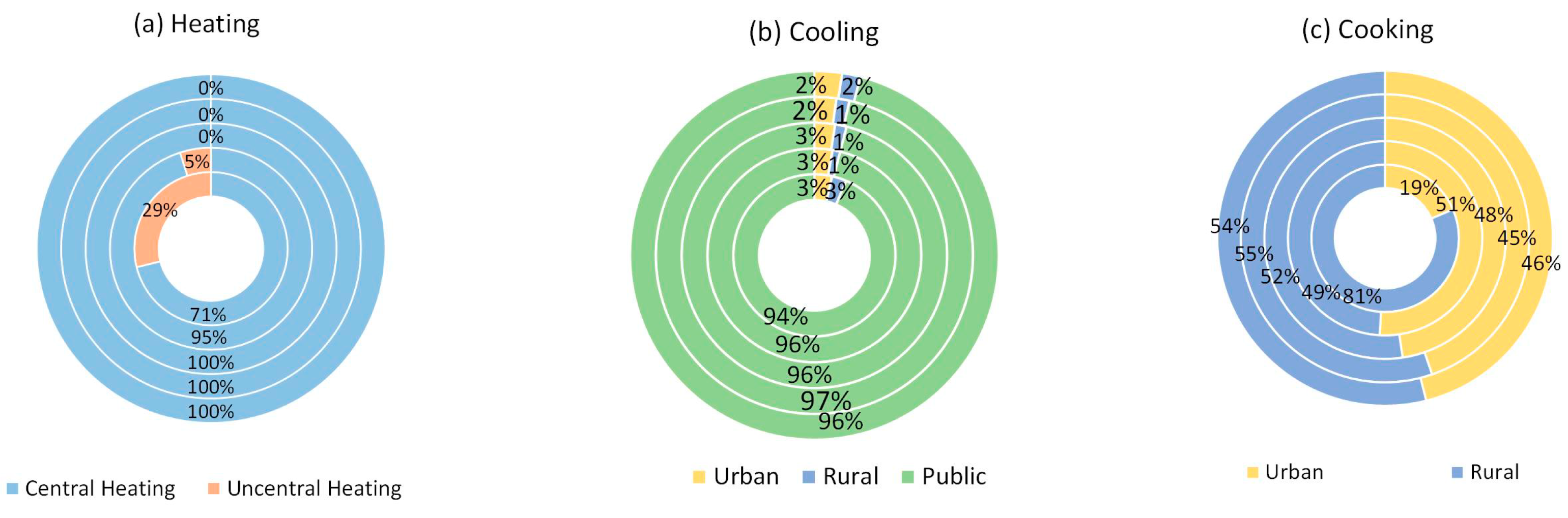
In consideration of the bottom–top process of LEAP, the macro and micro scales were considered. Therefore, five levels in the different scales were introduced in LEAP. In the first level, the buildings in the cold region were categorized into residential and public buildings. These building types have different carbon emissions. In residential buildings, carbon emissions come from heating, cooling, and cooking; in public buildings, emissions mostly come from air conditioning. In the second level, residential buildings were divided into urban and rural sectors, whereas public buildings were divided into offices, schools, hospitals, malls, hotels, and others. In the third level, heating, cooking, illumination, cooling, washing, boiling water, and others were the energy end-use activities performed in residential buildings. Heating, illumination, boiling water, and others were the energy end-use activities conducted in public buildings. In the fourth level, the energy end-use types were further classified depending on the different types of appliances. With respect to cooking activities, different cooking ranges led to different kinds of carbon emissions due to different energy types. For example, cooking ranges were operated by electricity, but cooking stoves consumed wood to function. In the fifth level, different energy types were consumed by different energy terminals. In this study, the eight common energy types were electricity, LPG, coal, bioenergy, solar, coal gas, fuel gas, and natural gas.

2.2. Carbon Emissions Accounting Method

According to the different energy end use and energy types, the carbon emissions were accounted for based on Equations (1)–(8) as follows.

C_H = P_CH × E_CH × f_c + P_NCH × E_NCH × f_c,

(1)

where C_H is the carbon emissions of heating in urban, Mt; P_CH represents the service ability of central heating; P_NCH represents the service ability of non-central heating; E_CH indicates the energy consumption of the central heating, E_NCH indicates the energy consumption of the non-central heating; and f_c is the carbon factors of coal.

$$C_{CK}={\displaystyle \sum _n{P}_{m,n,c}\times E_{m,n,c}\times f_m},$$

(2)

where C_CK is the carbon emissions of cooking, Mt; P_m,n,c represents the service ability of the nth terminal appliance in the cooking activity, year or m²; E_m,n,c indicates the energy consumption of the mth energy type from the nth terminal appliance in the cooking activity; and f_m is the carbon factors of the mth energy type.

$$C_I={\displaystyle \sum _n{P}_{n,I}\times E_{n,I}\times f_e},$$

(3)

where C_I is the carbon emissions of illumination, Mt; P_n,I represents the service ability of the nth terminal appliance in the illumination activity, year or m²; E_n,I indicates the energy consumption of the electricity from the nth terminal appliance in the illumination activity; and f_e is the carbon factors of electricity.

C_CL = P_r × E_r × f_e + P_a × E_a × f_e,

(4)

where C_CL is the carbon emissions of cooling, Mt; P_r represents the service ability of the refrigerator; P_a represents the service ability of the air conditioning; E_r indicates the energy consumption of the refrigerator; and E_a indicates the energy consumption of the air conditioning.

$$C_W={\displaystyle \sum _n{P}_{n,w}\times E_{n,w}\times f_e},$$

(5)

where C_W is the carbon emissions of washing, Mt; P_m,w represents the service ability of the nth terminal appliance in the washing activity, year or m²; and E_m,w indicates the energy consumption of the electricity from the nth terminal appliance in the washing activity.

$$C_{HW}={\displaystyle \sum _n{P}_{m,n,h}\times E_{m,n,h}\times f_m},$$

(6)

where C_HW is the carbon emissions of heating water in residential building, Mt; P_m,n,h represents the service ability of the nth terminal appliance in water heating, year or m²; and E_m,n,h indicates the energy consumption of the mth energy type from the nth terminal appliance in water heating.

$$C_O={\displaystyle \sum _n{P}_{m,n,o}\times E_{m,n,o}\times f_e},$$

(7)

where C_O is the carbon emissions from other sources, Mt; P_m,n,o represents the service ability of the nth terminal appliance in other activities, year or m²; and E_m,n,o indicates the energy consumption of the mth energy type from the nth terminal appliance in other activities.

C_T = C_H + C_CK + C_I + C_CL + C_W + C_HW + C_O,

(8)

where C_T is the total carbon emissions of the mth energy type from building sectors during the operation in cold regions, Mt.

3. Case Study

3.1. Research Zone

As one of the coldest provinces in China (as shown in Figure 3), Jilin has a heating period as long as six months per year, which leads to a substantial amount of carbon emissions from heating in residential buildings. According to the target of carbon emissions reduction set by Jilin, the carbon intensity would be reduced by 18.5% by 2020. Therefore, carbon emissions from the residential buildings should be the focus. In summary, Jilin province was regarded as the research area in the paper. Coupling the energy end-use activities with the energy types, the driving factors were identified and the peak value of the building sector in the operation stage was forecast. Based on the analysis, a pathway to reducing emissions was presented.

3.2. Data

The data on residential activities were sourced from Jilin Statistical Annual Book, covering the construction area, rate of central heating, and so on. The data on energy intensity were obtained from calculations performed in line with the energy policy and planning. The carbon coefficients of different energy types were obtained from the Chinese National Energy Board.

3.3. Scenario Setting

Scenario analysis supplied various possible programs according to strict ratiocination and assumptions about the development of society, the economy, industry, and technology. Considering the complexity of carbon emissions from the construction sector in Jilin, scenarios were set depending on the development of the economy, industrialization, and urbanization. According to the tendency of the influencing factors, four different scenarios with an emphasis on popularization of low-carbon policies and technologies were set in the paper, namely a baseline scenario, low-carbon scenario, energy-saving scenario, and energy-saving–low-carbon scenario.

3.3.1. Baseline Scenario (BAU)

In the BAU, 2014 was set as the baseline year, in strict accordance with the current status of low-carbon policy and technologies in the construction sector. The energy efficiency was found to be lower than under the other scenarios. Due to the higher level of living standards and consumption, the prevalence of household appliances increased under the scenario. In contrast, the carbon efficiency of household appliances was lower. Thus, the coefficients of energy structure and energy-saving technologies were set in conformance with existing energy-saving policy. Generally, BAU was reflective of the developmental tendency as well as carbon emissions, with the special energy-saving policy implications discounted.

3.3.2. Energy-Saving Scenario (ESS)

ESS was set according to the 13th “five-year plan.” Under the scenario, an improvement was made to the energy-saving policy. Meanwhile, technologies capable of achieving higher energy efficiency were applied in compliance with the BAU settings. Specifically, the construction area and population increased in comparison to the urbanization. The energy use technologies were developed properly. The energy efficiency of heating and cooking was boosted moderately and the energy intensity of coal and natural gas was increased marginally. To sum up, ESS demonstrated the state of development and emissions under the energy-saving policy.

3.3.3. Low-Carbon Scenario (LCS)

LCS was the most desirable scenario. Taking the sustainability of the social economy as well as the environment into account, the mode of economic growth experienced notable changes. The improvement made to technology stepped up. Under this scenario, the low-carbon policy was extremely significant in terms of energy, the economy, and technology. In particular, the process of urbanization, as well as the growth in building area and population, were slower than under the other scenarios. Owing to the vigorous development of low-carbon technology, the carbon efficiency of heating and cooking was enhanced substantially. The carbon intensity of coal and natural gas was reduced massively. The scenario demonstrated the maximum reduction that is achievable to balance the economy and emissions.

3.3.4. Energy-Saving–Low-Carbon Scenario (ELS)

In ELS, the coordination of economy and emissions was considered a crucial issue in the context of a low-carbon society. The trends of urbanization and a rising population decelerated. Meanwhile, the urban area was expanding at a slow pace. With regard to energy-saving technologies, the energy efficiency of cooking and heating was improved, but the intensity of coal and natural gas was lowered. This scenario modeled the coordination of the economy and emissions.

3.4. Coefficient Setting

3.4.1. Heating in Urban Areas

Heating in urban areas was split into two different parts, namely, central and decentralized heating. The portion of central heating will be above 90% by 2020 owing to the upgrade of heating systems through the “warm house” project. Meanwhile, heating area was predicted on the basis of growth patterns. Therefore, the percentage of central heating was set to 72% in 2020 and 100% in 2050 under BAU. Similarly, the proportion of central heating was 76%, 76%, and 100% in 2020 under ESS, ELS, and LCS, respectively. In addition, the indexes in 2050 under the three scenarios were invariably 100%.

In accordance with the 12th five-year plan on the energy savings of buildings, the energy-saving percentage was set to 75%, following the standard of energy-saving building design. As a result, the energy consumption per heating area was reduced to 2 kg standard coal in BAU. On the basis of BAU, the energy per heating area was lowered to 5–7 kg standard coal in EES and ELS. Energy consumption in ELS was reduced by 20% due to the increasingly stringent standards of energy saving and the upgrade of heating systems and energy structures. These settings are presented in

Table 1. Heating area and energy intensity of heating in urban areas.

		Heating Area (Million m2)	Central Heating Energy Intensity (tce/household·year)	Non-Central Heating Energy Intensity (tce */household·year)
Base Year	2014	662.24	0.01269	0.00945
BAU	2020	778.66	0.01251	0.01
	2030	893.08	0.0125	0.00905
	2050	851.46	0.01117	0.0074
ESS	2020	763.76	0.0123	0.0099
	2030	860.22	0.0123	0.0105
	2050	803.48	0.012	0.0097
ELS	2020	763.76	0.0123	0.0099
	2030	860.22	0.0107	0.0105
	2050	803.48	0.01	0.0097
LCS	2020	751.68	0.01026	0.00975
	2030	835.55	0.0096	0.01075
	2050	757.4	0.0107	0.01055

* tons of standard coal equivalent (tce) means the kilocalories from burning a ton of standard coal.

.

3.4.2. Cooking

The energy consumption from cooking was primarily contributed by a combination of everyday life in residential buildings and catering services in public buildings. Energy types included coal gas, natural gas, LPG, electricity, coal, and bioenergy. As the infrastructure improved, the energy types used in cooking changed remarkably. For example, energies with high efficiency, such as electricity and natural gas, were prevalent in urban household cooking because of the popularization of natural gas and electric furnaces. For rural households, coal, natural gas, and LPG substituted for bioenergy as the major energy types for cooking. In summary, the coefficient of cooking in urban areas was set in line with the Natural Gas Use Plan implemented in Jilin Province and under the Chinese Sustainable Energy Scenario in 2020. The specific data are presented in

Table 2. Proportions of different energy types used in urban and rural household cooking (%).

		Coal Gas		LPG		Natural Gas	Electricity	Bio-Gas	Bio-Energy
		Urban	Rural	Urban	Rural	Urban		Rural
Base Year	2014	5.02	25.38	35.75	9.69	17.64	13.85	12.3	51.32
BAU	2020	4	25.5	26	12	37	15	15	44
	2030	2.52	25.7	13.27	14.63	43.16	17.24	19.48	30.81
	2050	0.53	26.13	1.06	24.44	41.2	17.05	37.84	8.02
ESS	2020	3	22	22	25	46	15	10	39.5
	2030	1.23	21.67	9.3	26.67	52.08	17.93	14.8	23.65
	2050	0.0067	19.8	0.19	33.69	45.92	15.93	35.69	6.165
ELS	2020	3	22	22	25	46	15	10	39.5
	2030	1.23	21.67	9.3	26.67	52.08	17.93	14.8	23.65
	2050	0.0067	19.8	0.1887	33.69	45.92	15.93	35.69	6.165
LCS	2020	2	24.5	20	15	51	15	22	35
	2030	0.35	24.28	7.78	18.28	60.36	18.2	24.31	20.96
	2050	0.0035	23.56	0.1	31.46	48.13	24.98	37.55	5.46

. Then, the coefficient was assumed as the current status, as shown in

Table 3. Coefficient settings of energy intensity of cooking in public buildings (tce/m²·year).

		Coal Gas	LPG	Natural Gas
Base Year	2014	0.001	0.0014	0.0268
BAU	2020	0.00097	0.0014	0.0269
	2030	0.000923	0.0016	0.0312
	2050	0.000835	0.0011	0.034
ESS	2020	0.00094	0.0015	0.0277
	2030	0.00085	0.0016	0.0306
	2050	0.0007	0.0006	0.0228
ELS	2020	0.00094	0.0015	0.0277
	2030	0.00085	0.0016	0.0306
	2050	0.0007	0.0006	0.0228
LCS	2020	0.00093	0.0015	0.028
	2030	0.00082	0.0009	0.025
	2050	0.00065	0.00032	0.0169

, due to a shortage of detailed energy consumption data for cooking in public buildings.

3.4.3. Illumination

Recently, the proportion of energy consumption taken up by illumination has been rising incrementally in buildings, especially public ones. Therefore, limiting the carbon emissions caused by illumination was a priority in this study. In accordance with the design standard for illumination in buildings, the current energy intensity and illumination activities in buildings were explored, along with the disparities between urban and rural areas.

Light in buildings was categorized into normal and energy-saving light. In consideration of the current process of promoting energy-saving light in Jilin, the extent of popularization for energy-saving light was predicted to show an increasing trend. In residential buildings, the popularity of energy-saving light was expected to reach 45%, 52%, 59%, and 59% in 2020 under BAU, EES, ELS, and LCS, respectively. The same coefficient was 84%, 84%, and 85%, respectively. In comparison with urban areas, the popularity of energy-saving light in rural areas was found to be noticeably low. The proportion of energy-saving light was expected to be 23%, 26%, 26%, and 30% in 2020 and 47%, 51%, 51%, and 52% in 2050 under BAU, EES, ELS, and LCS, respectively. In public buildings, the proportion of energy-saving light was anticipated to reach 50%, 58%, 58%, and 65% in 2020 and 86%, 89%, 89%, and 95% in 2050 under the four scenarios. The detailed coefficients are shown in

Table 4. Coefficient settings of energy intensity of illumination in buildings (tce/m²·year).

		Normal Light			Energy-Saving Light
		Urban	Rural	Public	Urban	Rural	Public
Base Year	2014	0.0294	0.0106	0.0009	0.0088	0.0032	0.0003
BAU	2020	0.0332	0.012	0.00092	0.01	0.0036	0.000301
	2030	0.037	0.015	0.001	0.009	0.0038	0.00033
	2050	0.0407	0.017	0.00107	0.0085	0.004	0.00035
ESS	2020	0.0324	0.0117	0.00094	0.0065	0.0023	0.00031
	2030	0.0394	0.013	0.001	0.006	0.0022	0.00033
	2050	0.0464	0.0168	0.0008	0.005	0.0021	0.00027
ELS	2020	0.0324	0.0117	0.00094	0.0065	0.0023	0.00031
	2030	0.0394	0.013	0.001	0.006	0.0022	0.00033
	2050	0.0464	0.0168	0.0008	0.005	0.0021	0.00027
LCS	2020	0.0316	0.0115	0.00096	0.003	0.002	0.00032
	2030	0.04	0.013	0.00086	0.0028	0.0018	0.00029
	2050	0.0484	0.0165	0.00058	0.0025	0.0017	0.00019

.

3.4.4. Cooling in Residential Buildings

Refrigerators are considered the most commonly used appliance, and represent high levels of energy consumption. As revealed by the Jilin Statistical Yearbook, 91.13 refrigerators were found for every 100 urban households, and 89.37 refrigerators were found for every 100 rural households in 2014. Based on the current rate, refrigerator penetration was supposed to reach 100% among urban and rural households under the four scenarios in 2020. Our previous research indicated that appliances with high levels of energy efficiency have gained in popularity over the recent years. Therefore, obsolete refrigerators should all be replaced by 2020. The investigation revealed that outdated refrigerators could consume as much as 1.2 kwh per day in contrast to 0.8 kwh per day for energy-saving refrigerators. In consideration of the effect of new technology and energy consumption standards on energy efficiency, the energy efficiency of refrigerators has not changed significantly. Detailed data are given in

Table 5. Coefficient settings of energy intensity of refrigerators (tce/set·year).

		Older Refrigerator	Energy-Saving Refrigerator
Base Year	2014	0.054	0.04
BAU	2020	0.054	0.04
	2030	0.054	0.039
	2050	0.054	0.038
ESS	2020	0.054	0.038
	2030	0.054	0.037
	2050	0.054	0.036
ELS	2020	0.054	0.038
	2030	0.054	0.037
	2050	0.054	0.036
LCS	2020	0.054	0.036
	2030	0.054	0.035
	2050	0.054	0.034

. In addition to refrigerators, air conditioners are another major cooling appliance. On the basis of the results obtained from previous research, the energy consumption coefficients are presented in

Table 6. Coefficient settings of energy intensity of air conditioning (tce/household·year).

	Year	Energy Intensity
Base Year	2014	0.017
BAU	2020	0.0178
	2030	0.0196
	2050	0.0206
ESS	2020	0.0178
	2030	0.019
	2050	0.016
ELS	2020	0.0178
	2030	0.019
	2050	0.016
LCS	2020	0.0179
	2030	0.0162
	2050	0.0133

.

3.4.5. Washing in Residential Buildings

As demonstrated by the Jilin Statistical Yearbook, 95 washing machines were found for every 100 urban households, whereas 85.61 were found for every 100 rural households in 2014. Roller washing machines are the major type of washing machine for household use. The proportion of roller washing in urban areas reached 60%, in comparison with 80% in rural areas. Washing machines were classified into roller and impeller types. In view of the different work modes between the two types, the energy consumption of a roller one was assumed to be 750 W per working cycle, and 160 working cycles were assumed to occur in a year under BAU. The working cycle was raised by 40, 40, and 45 under EES, ELS, and LCS based on BAU, respectively. For impeller washing machines, the energy consumption was assumed to be 120 W per working cycle, and 160 working cycles were presumed to occur in a year under BAU. The working cycle of an impeller one was identical to that of a roller one. The detailed coefficients are listed in

Table 7. Coefficient settings of energy intensity of washing machines (tce/household·year).

		Roller Washing Machine	Impeller Washing Machine
Base Year	2014	0.0393	0.0024
BAU	2020	0.0393	0.0024
	2030	0.0417	0.002448
	2050	0.044	0.00255
ESS	2020	0.0442	0.002499
	2030	0.0443	0.002601
	2050	0.0445	0.002703
ELS	2020	0.0442	0.002499
	2030	0.0443	0.002601
	2050	0.0445	0.002703
LCS	2020	0.0445	0.0026
	2030	0.0446	0.0027
	2050	0.0448	0.0028

.

3.4.6. Heating Water in Residential Buildings

The investigation showed that energy consumption for heating water constituted 20% of the total amount of energy consumed in buildings. As living standards improve, the demand for heated water increases. At present, electrical and solar heaters are the two major types of water heaters. In accordance with the Jilin Statistical Yearbook, 68.28 water heaters were available for every 100 urban households, whereas 9.91 were available for 100 rural households in 2014. The working period of a water heater was assumed to be 365 and 270 days annually in urban and rural areas, respectively. The amount of energy consumed by water heaters was 2 kw daily. Solar heaters were not used extensively in Jilin Province due to the long cold period. Moreover, a solar heater was unlikely to contribute to carbon emissions. Thus, solar heaters were discounted from the calculations. The tendency of water heating in buildings was extrapolated on the basis of the energy planning in Jilin Province. In BAU, the growth of electric heating was faster pace than that in the other three scenarios. By contrast, solar heating was promoted due to the improvement in clean energy under ESS, ELS, and LCS. The detailed data are presented in

Table 8. Coefficient settings of proportion and energy intensity of water heaters.

		Set per 100 households		Energy Intensity (tce/set)
		Urban	Rural	Urban	Rural
Base Year	2014	68.28	9.91	0.0897	0.0664
BAU	2020	92.7	15.63	0.0897	0.0664
	2030	100	29.33	0.0898	0.068
	2050	100	38.02	0.09	0.07
ESS	2020	93.15	22.5	0.0897	0.0664
	2030	100	46.37	0.0898	0.068
	2050	100	47.15	0.09	0.07
ELS	2020	93.15	22.5	0.0897	0.0664
	2030	100	46.37	0.0898	0.068
	2050	100	47.15	0.09	0.07
LCS	2020	100	30	0.0897	0.0664
	2030	100	74.34	0.0898	0.068
	2050	100	59.27	0.09	0.07

.

3.4.7. Other Electrical Appliances

As technology and the economy have advanced, new types of electric appliances, such as televisions and computers in residential buildings and printers and projectors in public buildings, have emerged. The emergence of these appliances has triggered an increase in energy consumption. In view of the heterogeneity in the energy consumption level of appliances, the activity level of electric appliances was uniformly set to 100%. The energy intensity of the baseline year was denoted as the ratio of energy consumption to the activity level. On the basis of the energy intensity under BAU, the energy intensity under the other three scenarios was restricted in growth due to the limitations imposed by the prevalence of energy-saving appliances and energy-saving standards. The detailed coefficients are shown in

Table 9. Coefficient settings of energy intensity of other appliances (tce/household·year).

	Year	Energy Intensity
Base Year	2014	0.0046
BAU	2020	0.005
	2030	0.0055
	2050	0.0058
ESS	2020	0.0051
	2030	0.0055
	2050	0.0045
ELS	2020	0.0051
	2030	0.0055
	2050	0.0045
LCS	2020	0.005148
	2030	0.00466
	2050	0.0031

.

4. Results and Discussion

4.1. Predicting the Peak Value

As indicated by Figure 4, the peak carbon emissions from buildings during the operation period in Jilin Province were predicted with LEAP under the four scenarios. The results demonstrated that the peak value was between 37.17 and 48.49 Mt under the four scenarios. The earliest peak time and the most insignificant peak value were found under LCS. The peak value, which occurred in 2025, was shown to be 37.17 Mt. Meanwhile, the second-highest one was found to be 42.06 Mt in 2030 under ELS. The peak value under ESS reached 45.19 Mt in 2035. On the contrary, with the latest peak time and the highest peak value, 48.48 Mt was shown to occur in 2040 under BAU.

Therefore, the difference in peak time and value was apparent as the scenario settings differed. In contrast to BAU, the population size under ESS increased. Despite this finding, energy-saving technology and energy efficiency were enhanced due to the enforcement of an energy-saving policy. Meanwhile, the expansion of urbanization slowed down. The peak time under ESS was five years in advance, and the peak value was 3.3 Mt lower under BAU due to the aforementioned settings. For ELS, the roll-out of the energy-saving policy was reinforced on the basis of ESS. Meanwhile, a low-carbon society was achieved. Population growth and urbanization were restricted, and the speed of building area growth was reduced. The key was the improvement of energy technologies, which enhanced energy efficiency for heating, cooking, cooling, and other energy consumption activities. Therefore, the peak time under ELS was 10 years ahead of that under BAU. The reduction of the peak value under BAU was 6.43 Mt. Compared with ESS and ELS, LCS represented the ideal scenario with the lowest carbon level. Under LCS, controlling carbon emissions was emphasized with the development in social economy discounted. The peak time under LCS was 15 years in advance of that under BAU. Meanwhile, the peak value was merely 76.65% of that under BAU. Despite the peak time and value under LCS being the best among the four scenarios, this scenario was unrealistic for developing regions in middle to late industrialization and urbanization, such as Jilin Province. Regarding the economy, restricting the development of the social economy for carbon emissions reduction failed to satisfy the requirement of improving living standards. In consideration of energy-saving policies and technologies, the ideal low-carbon society under LCS in Jilin Province could not be realized in the foreseeable future. In summary, ESS and ELS were practical scenarios in Jilin Province. Nevertheless, a detailed pathway to reducing carbon emissions was deemed necessary for exploration in the next section.

4.2. Identifying the Driving Factors

Generally, carbon emissions from heating in buildings in the cold regions contribute the largest total percentage, followed by cooling and cooking. As shown in Figure 5, the value of carbon emissions from heating ranged between 20 and 30 Mt, accounting for 54–62% of the total emissions. High emissions were associated with the huge consumption of coal during the long heating period in cold regions. Cooling and cooking had similar emissions of 6–8 Mt, which accounted for 11–20% of total emissions. For the other activities, emissions from illumination and washing were lower than those from heating water due to the substantial demand for hot water in the long winter. In particular, heating, cooling, and cooking discharged 23.45, 7.93, and 7.27 Mt of carbon, and contributed 55.74%, 18.86%, and 17.29% of total emissions, respectively, under ELS. By contrast, other activities, such as illumination and washing, comprised less than 10%. Over 90% of total carbon emissions from buildings in the cold region were discharged by heating, cooling, and cooking. On the basis of this finding, the three main activities were considered the key factors driving carbon emissions reduction.

Figure 6a shows that the carbon emissions from heating in Jilin Province were 29.82, 26.81, 23.45, and 20.07 Mt under BAU, ESS, ELS, and LCS, respectively. On the basis of the distinction in heating methods, heating was categorized into centralized and decentralized heating. The proportion of central heating was 71.11% in 2014 (the baseline). A comparison of the four scenarios showed that the percentage of central heating was 95% at peak time under BAU, but 100% under the remaining three scenarios. The gap in central heating between BAU and the other three scenarios led to huge emissions under BAU. The results demonstrated that the structure of heating could reduce emissions. Moreover, decelerating the growth of urbanization, restricting the increase in building area, popularizing energy-saving technologies, and enhancing heating efficiency were effective at reducing the carbon emissions from heating.

For cooling, in Jilin Province, air conditioning in public buildings and refrigerators in residential buildings were the major activities. The emissions from air conditioning in public buildings were approximately 96% of the total emissions from cooling activities. This result is illustrated in Figure 6b. Air conditioning is not common in residential buildings in Jilin Province because the houses tend to have thick walls against the cold weather, so a large proportion of carbon emissions was from the air conditioning in public buildings.

Regarding cooking, there were different furnaces and energy types used in urban and rural areas. The results revealed that cooking in rural areas contributed 81.41% of total emissions. The use of furnaces and firewood in rural residential buildings resulted in large emissions. The results showed that the carbon emissions from cooking activities accounted for 50% of total emissions in buildings under the four scenarios. Therefore, the expansion of urbanization and population led to an increase in carbon emissions from cooking. However, the upgrade of furnaces and the enhancement of energy efficiency were major approaches to reducing carbon emissions. Therefore, Figure 6c shows that carbon emissions from rural cooking were reduced by the adjustment on the energy structure through urbanization.

4.3. Evaluating the Impact of Driving Factors

A sensitivity analysis was adopted to quantitatively assess the impact of driving factors. Taking ELS as an example, 32 driving factors affected the carbon emissions of buildings in the cold regions.

Table 10. Sensitive analysis results of positive driving factors.

Driving Factors		Type	Variation (Mt)	Proportion (%)	Total (%)
Urban scale	Households	Urban	1.55	17.41	17.41
Heating	Heating area	Urban	1.95	21.91	35.51
	Intensity of central heating		1.21	13.61
Cooling	Building area	Public	1.98	22.21	31.10
	Intensity of air conditioner	Public	0.77	8.58
	Intensity of energy-saving refrigerator	Urban	0.02	0.20
		Rural	0.01	0.09
	Intensity of older refrigerator	Rural	0.00	0.02
Cooking	Cooking structure	Urban	0.59	6.60	14.07
	Intensity of natural gas stove	Urban	0.31	3.43
	Intensity of LPG stove	Urban	0.02	0.18
		Rural	0.12	1.38
	Intensity of wood burning stove	Rural	0.22	2.48
Illumination	Ratio of normal light to energy-saving light	Urban	0.02	0.18	0.85
		Rural	0.00	0.03
		Public	0.03	0.30
	Intensity of normal light	Urban	0.00	0.04
		Rural	0.00	0.02
		Public	0.01	0.08
	Intensity of energy-saving light	Urban	0.00	0.03
		Rural	0.00	0.02
		Public	0.01	0.13
Heating water	Intensity of electrical heater	Urban	0.04	0.45	0.53
		Rural	0.01	0.08
Washing	Ratio of roller washing machines to impeller washing machines	Urban	0.02	0.22	0.53
		Rural	0.01	0.11
	Intensity of roller washing machine	Urban	0.01	0.10
		Rural	0.01	0.06
	Intensity of impeller washing machine	Urban	0.00	0.01
		Rural	0.00	0.02

lists the 30 driving factors with positive effects. However, only two driving factors, namely, the proportion of urban buildings and the structure of rural cooking, exerted an adverse impact on carbon emissions. In the case of the 10% rise in the proportion of urban buildings, the peak value of carbon emissions decreased by 0.55 Mt. Similarly, the 10% of firewood furnaces, which was replaced by LPG furnaces, reduced carbon emissions by 0.13 Mt.

The positive factors were split into two parts. The first included population size and urban size. The sensitivity analysis revealed that the 10% rise in total number of households increased carbon emissions by 1.55 Mt, representing 17.41% of the total change in carbon emissions. The second part included activities during the operation period in buildings. Heating, cooling, and cooking made the most noticeable impact on carbon emissions, which is consistent with the results in Section 4.2. Meanwhile, heating was the top-ranked factor, accounting for 35.51% of the total change in carbon emissions. Therefore, the change in heating area caused 21.9% of the total change in peak carbon emissions. The intensity of central heating caused 13.61% of the change in carbon emissions. Cooling was the second most evident influencing factor, with 31.10% of the total change made to carbon emissions. The area of public buildings contributed a 22.21% effect to carbon emissions. Meanwhile, the reduction in the intensity of emissions resulting from improvements made to technology contributed 8.58% to carbon emissions reduction. Other cooling activities, such as refrigeration in urban and rural areas, comprised 0.31% of the total impact. Cooking was the third driving factor in the reduction of carbon emissions. Cooking activities in buildings contributed 14.07% to the total decline in carbon emissions. The change made to urban cooking structures reduced the peak value by 6.6%. Meanwhile, the improvement made to energy efficiency caused by technological advances contributed 7.47% to emissions reduction. In comparison with the top three activities, other activities, such as illumination, washing, and heating water, had a limited impact on carbon emissions (0.85%, 0.53%, and 0.53%, respectively).

4.4. Discussion

The results in Section 4.2 and Section 4.3 show that rural households made a positive contribution to the reduction of carbon emissions (by 17.41%). On the contrary, urban residential buildings had a negative impact on carbon emissions. Therefore, in view of the above two factors, urban size was considered a leading factor in carbon emissions. Among the 30 negative factors, heating, cooling, and cooking comprised the top three. In summary, our research into reducing carbon emissions revealed four major driving factors, namely, urban size, heating, cooling, and cooking, and involved seven indices, namely, households in buildings, ratio of central heating, carbon intensity of central heating, public building area, carbon intensity of air conditioners, cooking structure, and carbon intensity of furnaces. Therefore, a pathway to reducing carbon emissions in cold regions was presented on the basis of the above indexes.

4.4.1. The Best Pathway: BAU-ELS

In accordance with the target for reducing carbon emissions in Jilin Province, the peak time should be earlier than 2030, and the peak value should be no more than 42.06 Mt. Efforts should be made to ensure that this target is achieved.

From the perspective of policy, the slow growth of population, urbanization, and building area should be considered. The number of residential buildings should be 93,321.48 million households and 90,970.17 million households in 2030 and 2050, respectively. Central heating should be installed in the entire Jilin Province by 2030. Reducing the consumption of coal and firewood will increase the percentage of natural gas applied to cooking by 52.08% and 45.92% by 2030 and 2050, respectively.

As shown in Figure 7, the carbon intensity of central heating will reach 0.0107 and 0.01 tce/m² by 2030 and 2050, respectively, through the development of energy end-use technologies. The improvements made to cooking technology have triggered a change in the carbon intensity of LPG and natural gas. By 2030 and 2035, the intensity of LPG and natural gas will reach 0.163 and 0.161 tce/household·year and 0.62 and 0.65 tce/household·year, respectively. Furthermore, energy-saving appliances, such as lights, washing machines, and water heaters, should be utilized widely in the future. In summary, for controlling of growth in urbanization, low-carbon technologies should be promoted.

4.4.2. Pathway 2: BAU-ESS

In accordance with the ESS scenario, peak emissions are expected in 2035, with a value of 45.19 Mt. In keeping with government policy, urbanization was pushed increasingly. The number of households in residential buildings will be 9,520,338 and 9,331,715 by 2035 and 2050, respectively. The proportion of decentral heating will be reduced. Therefore, central heating will cover the entire province from 2030. The substitution of coal and firewood with natural gas and LPG caused a rise in the percentage of natural gas in cooking structure: 52.08% and 45.92% of energy consumption in cooking activities will be natural gas by 2030 and 2050, respectively.

Improvement in energy end use was the key aim of ESS. The carbon intensity of heating was 0.0123 and 0.012 tce/m², respectively, due to advanced technology. In terms of cooking structure, the carbon intensity of LPG increased to 0.163 and 0.161 tce/household·year. Similarly, the carbon intensity of natural gas reached 0.62 and 0.65 tce/household·year.

4.4.3. Pathway 3: BAU-LCS

Under LCS, the peak time was 2025, with a value of 37.17 Mt. From the perspective of policy, the population growth decelerated, and a low-carbon society was promoted. Urbanization was significantly lower than under the other three scenarios. The number of residential buildings was expected to be 9,161,283 and 8,837,033 by 2030 and 2050, respectively. The ratio of central heating is expected to reach 100% by 2030 due to the decline in the percentage of decentralized heating. Coal and firewood furnaces will be replaced by LPG and natural furnaces. The ratio of natural gas in cooking activities will increase on the basis of the aforementioned replacement. Natural gas accounts for 60.36% and 48.13% of the total energy consumption in cooking in the two scenarios. Low-carbon technologies enhance the efficiency of energy end use in heating and cooking. The carbon intensity of heating will reach 0.00096 and 0.01 tce/m² by 2030 and 2050, respectively. For cooking, the intensity of LPG will reach 0.117 and 0.115 tce/household·year by 2030 and 2050, respectively. The carbon intensity of natural gas will increase to 0.66 and 0.65 tce/household·year, respectively.

5. Conclusions

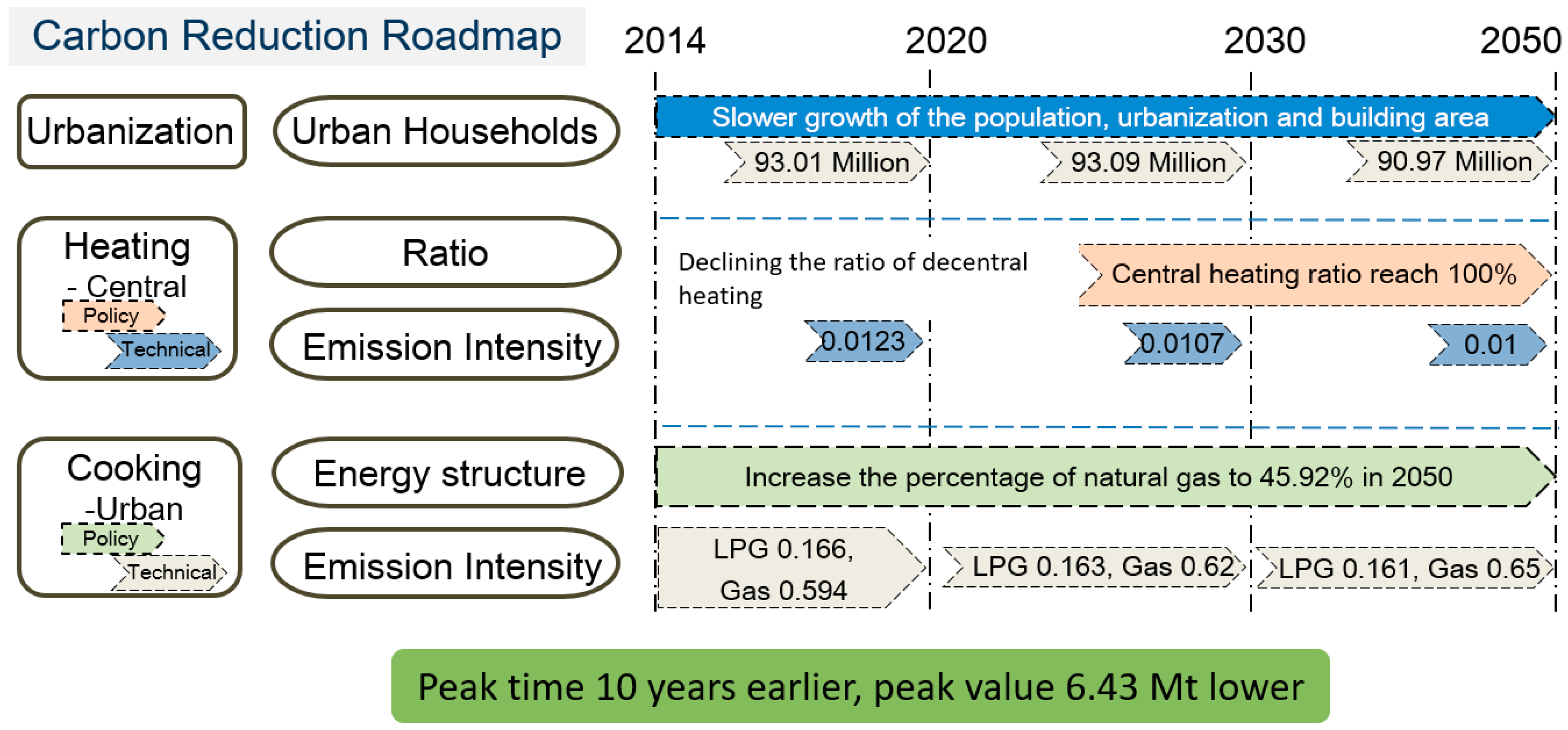
In view of the growing carbon emissions from buildings during operation in cold regions, LEAP, sensitivity analysis, and scenario analysis were used to forecast the peak value, identify the driving factors, and search for a way to reduce emissions. The results revealed that the peak and peak time varied between the scenarios. On the basis of the balance between development and low carbon, ELS was regarded as the optimal scenario. Under ELS, the peak time was 2030 according to the national target. After comparing the four scenarios, heating was found to be the top-ranking driving factor of carbon emissions in the cold region. Heating contributed 20–30 Mt carbon emissions, and accounted for 54–62% of total emissions in buildings. Cooling and cooking were the second-highest carbon-emitting activities, with a value of 6–8 Mt. The emissions from cooling and cooking comprised 11–20% of the total emissions. The results obtained from the sensitivity analysis indicated that two negative indexes refer to urban size, and 30 positive indexes had a relationship with urban size and activities such as heating, cooking, and cooling. After combining policy and technology, pathways to reducing carbon emissions under different scenarios were suggested. In view of the assessment of carbon emissions based on the number of households, percentages of central heating, carbon intensity of central heating, public building area, carbon intensity of air conditioning, cooking structure, and carbon intensity of furnaces, the BAU-ELS pathway was considered to offer the optimal balance between development and low carbon.

No optimization function was available in the LEAP model. The optimal scenario could not be obtained from LEAP. Thus, a scenario analysis for identifying the reduction pathway must be introduced. In our future work, the optimization model may be introduced quantitatively into LEAP for the optimal reduction pathway. In addition, with Jilin Province representing a vast cold region in China, uncertainty of coefficients exists in the study. Without considering the geographic heterogeneity in carbon emissions, the relationship between carbon emissions and the cold was not discussed in our research, but it will be tackled in our next work.

References

1. Wang, L.; Chen, X.; Wang, L.; Sun, S.; Tong, L.; Yue, X.; Yin, S.; Zheng, L. Contribution from Urban Heating to China’s 2020 Goal of Emission Reduction. Environ. Sci. Technol. 2011, 45, 4676–4681. [Google Scholar] [CrossRef] [PubMed]
2. He, Q.; Jiang, X.; Gouldson, A.; Sudmant, A.; Guan, D.; Colenbrander, S.; Xue, T.; Zheng, B.; Zhang, Q. Climate change mitigation in Chinese megacities: A measures-based analysis of opportunities in the residential sector. Appl. Energy 2016, 184, 769–778. [Google Scholar] [CrossRef]
3. Yang, X.; Hu, M.; Wu, J.; Zhao, B. Building-information-modeling enabled life cycle assessment, a case study on carbon footprint accounting for a residential building in China. J. Clean. Prod. 2018, 183, 729–743. [Google Scholar] [CrossRef]
4. Chau, C.K.; Leung, T.; Ng, W. A review on Life Cycle Assessment, Life Cycle Energy Assessment and Life Cycle Carbon Emissions Assessment on buildings. Appl. Energy 2015, 143, 395–413. [Google Scholar] [CrossRef]
5. Xian, Y.; Yang, K.; Wang, K.; Wei, Y.M.; Huang, Z. Cost-environment efficiency analysis of construction industry in China: A materials balance approach. J. Clean. Prod. 2019, 221, 457–468. [Google Scholar] [CrossRef]
6. Yu, L.; Wang, S.; Lu, Q.; Feng, G. Sensitivity Analysis of Existing Residential Building Energy Consumption Influencing Factors in Cold Regions. Procedia Eng. 2016, 146, 196–203. [Google Scholar] [CrossRef] [Green Version]
7. Asaee, S.R.; Sharafian, A.; Herrera, O.E.; Blomerus, P.; Mérida, W. Housing stock in cold-climate countries: Conversion challenges for net zero emission buildings. Appl. Energy 2018, 217, 88–100. [Google Scholar] [CrossRef]
8. You, F.; Hu, D.; Zhang, H.; Guo, Z.; Zhao, Y.; Wang, B.; Yuan, Y. Carbon emissions in the life cycle of urban building system in China—A case study of residential buildings. Ecol. Complex. 2011, 8, 201–212. [Google Scholar] [CrossRef]
9. Fan, J.-L.; Yu, H.; Wei, Y.M. Residential energy-related carbon emissions in urban and rural China during 1996–2012: From the perspective of five end-use activities. Energy Build. 2015, 96, 201–209. [Google Scholar] [CrossRef]
10. Torregrosa-Jaime, B.; Gonzalez, B.; Martínez, P.J.; Payá-Ballester, G. Analysis of the Operation of an Aerothermal Heat Pump in a Residential Building Using Building Information Modelling. Energies 2018, 11, 1642. [Google Scholar] [CrossRef]
11. Ma, M.; Cai, W. What drives the carbon mitigation in Chinese commercial building sector? Evidence from decomposing an extended Kaya identity. Sci. Total Environ. 2018, 634, 884–899. [Google Scholar] [CrossRef] [PubMed]
12. Niu, S.; Zhang, X.; Zhao, C.; Niu, Y. Variations in energy consumption and survival status between rural and urban households: A case study of the Western Loess Plateau, China. Energy Policy 2012, 49, 515–527. [Google Scholar] [CrossRef]
13. Sadri, A.; Ardehali, M.; Amirnekooei, K. General procedure for long-term energy-environmental planning for transportation sector of developing countries with limited data based on LEAP (long-range energy alternative planning) and EnergyPLAN. Energy 2014, 77, 831–843. [Google Scholar] [CrossRef]
14. Nejat, P.; Jomehzadeh, F.; Taheri, M.M.; Gohari, M.; Majid, M.Z.A. A global review of energy consumption, CO2 emissions and policy in the residential sector (with an overview of the top ten CO2 emitting countries). Renew. Sustain. Energy Rev. 2015, 43, 843–862. [Google Scholar] [CrossRef]
15. Fan, F.; Lei, Y. Index Decomposition Analysis on Factors Affecting Energy-Related Carbon Dioxide Emissions from Residential Consumption in Beijing. Math. Probl. Eng. 2017, 2017, 1–14. [Google Scholar] [CrossRef] [Green Version]
16. Mavromatidis, G.; Orehounig, K.; Richner, P.; Carmeliet, J. Corrigendum to “A strategy for reducing CO2 emissions from buildings with the Kaya identity—A Swiss energy system analysis and a case study”. Energy Policy 2016, 98, 470. [Google Scholar] [CrossRef]
17. Ma, M.; Cai, W.; Cai, W. Carbon abatement in China’s commercial building sector: A bottom-up measurement model based on Kaya-LMDI methods. Energy 2018, 165, 350–368. [Google Scholar] [CrossRef]
18. Lin, B.; Liu, H. CO2 emissions of China’s commercial and residential buildings: Evidence and reduction policy. Build. Environ. 2015, 92, 418–431. [Google Scholar] [CrossRef]
19. Liu, Z.G.; Wang, S.S.; Liu, J.Y.; Liu, F.; Fu, X.L. Analysis of factors affecting CO2 emissions by civil buildings in China’s urban areas. Int. J. Low Carbon Technol. 2015, 10, 460–463. [Google Scholar] [CrossRef]
20. Jiang, J. China’s urban residential carbon emission and energy efficiency policy. Energy 2016, 109, 866–875. [Google Scholar] [CrossRef]
21. Ma, M.; Yan, R.; Cai, W. An extended STIRPAT model-based methodology for evaluating the driving forces affecting carbon emissions in existing public building sector: Evidence from China in 2000–2015. Nat. Hazards 2017, 89, 741–756. [Google Scholar] [CrossRef]
22. Wu, C.B.; Huang, G.H.; Xin, B.G.; Chen, J.K. Scenario analysis of carbon emissions’ anti-driving effect on Qingdao’s energy structure adjustment with an optimization model, Part Ⅰ: Carbon emissions peak value prediction. J. Clean. Prod. 2018, 172, 466–474. [Google Scholar] [CrossRef]
23. Shimoda, Y.; Yamaguchi, Y.; Okamura, T.; Taniguchi, A.; Yamaguchi, Y. Prediction of greenhouse gas reduction potential in Japanese residential sector by residential energy end-use model. Appl. Energy 2010, 87, 1944–1952. [Google Scholar] [CrossRef]
24. Tan, X.; Lai, H.; Gu, B.; Zeng, Y.; Li, H. Carbon emission and abatement potential outlook in China’s building sector through 2050. Energy Policy 2018, 118, 429–439. [Google Scholar] [CrossRef]
25. Wan, K.; Yik, F. Building design and energy end-use characteristics of high-rise residential buildings in Hong Kong. Appl. Energy 2004, 78, 19–36. [Google Scholar] [CrossRef]
26. De Lauretis, S.; Ghersi, F.; Cayla, J.M. Energy consumption and activity patterns: An analysis extended to total time and energy use for French households. Appl. Energy 2017, 206, 634–648. [Google Scholar] [CrossRef] [Green Version]
27. Howard, B.; Parshall, L.; Thompson, J.; Hammer, S.; Dickinson, J.; Modi, V. Spatial distribution of urban building energy consumption by end use. Energy Build. 2012, 45, 141–151. [Google Scholar] [CrossRef]
28. Thuy, V.T.H.; Limmeechokchai, B. Analyses of Energy use and CO2 Emission in Residential Sector: Case Studies in Thailand and Vietnam. Energy Procedia 2015, 79, 290–295. [Google Scholar] [CrossRef]
29. Jeong, Y.S. Assessment of Alternative Scenarios for CO2 Reduction Potential in the Residential Building Sector. Sustainability 2017, 9, 394. [Google Scholar] [CrossRef]
30. Chaichaloempreecha, A.; Winyuchakrit, P.; Limmeechokchai, B. Long-term energy savings and GHG mitigations in Thailand’s building sector: Impacts of energy efficiency plan. Energy Procedia 2017, 138, 847–852. [Google Scholar] [CrossRef]
31. Siller, T.; Kost, M.; Imboden, D. Long-term energy savings and greenhouse gas emission reductions in the Swiss residential sector. Energy Policy 2007, 35, 529–539. [Google Scholar] [CrossRef]
32. Bjørnstad, O.N.; Grenfell, B.T. Noisy Clockwork: Time Series Analysis of Population Fluctuations in Animals. Science 2001, 293, 638–643. [Google Scholar] [CrossRef] [PubMed] [Green Version]
33. Taniguchi, A.; Inoue, T.; Otsuki, M.; Yamaguchi, Y.; Shimoda, Y.; Takami, A.; Hanaoka, K. Estimation of the contribution of the residential sector to summer peak demand reduction in Japan using an energy end-use simulation model. Energy Build. 2016, 112, 80–92. [Google Scholar] [CrossRef]
34. Leibowicz, B.D.; Lanham, C.M.; Brozynski, M.T.; Vázquez-Canteli, J.R.; Castejón, N.C.; Nagy, Z. Optimal decarbonization pathways for urban residential building energy services. Appl. Energy 2018, 230, 1311–1325. [Google Scholar] [CrossRef]
Figure 1. The technical roadmap.
Sustainability 11 04540 g001
Figure 2. The structure of LEAP to predict carbon emissions.
Sustainability 11 04540 g002
Figure 3. Map of the study area.
Sustainability 11 04540 g003
Figure 4. The predictions of carbon emissions trend in Jilin Province.
Sustainability 11 04540 g004
Figure 5. Carbon emissions of different activities at peak time.
Sustainability 11 04540 g005
Figure 6. Carbon emissions percentage of different services in base year and peak time (from the inside to the outside: base year 2014, BAU 2040, ESS 2035, ELS 2030, and LCS 2025).
Sustainability 11 04540 g006
Figure 7. Carbon reduction roadmap: BAU-ELS.
Sustainability 11 04540 g007