College Students’ Shared Bicycle Use Behavior Based on the NL Model and Factor Analysis

Abstract
1. Introduction
2. Data and Methods
2.1. Data Acquisition and Travel Characteristics
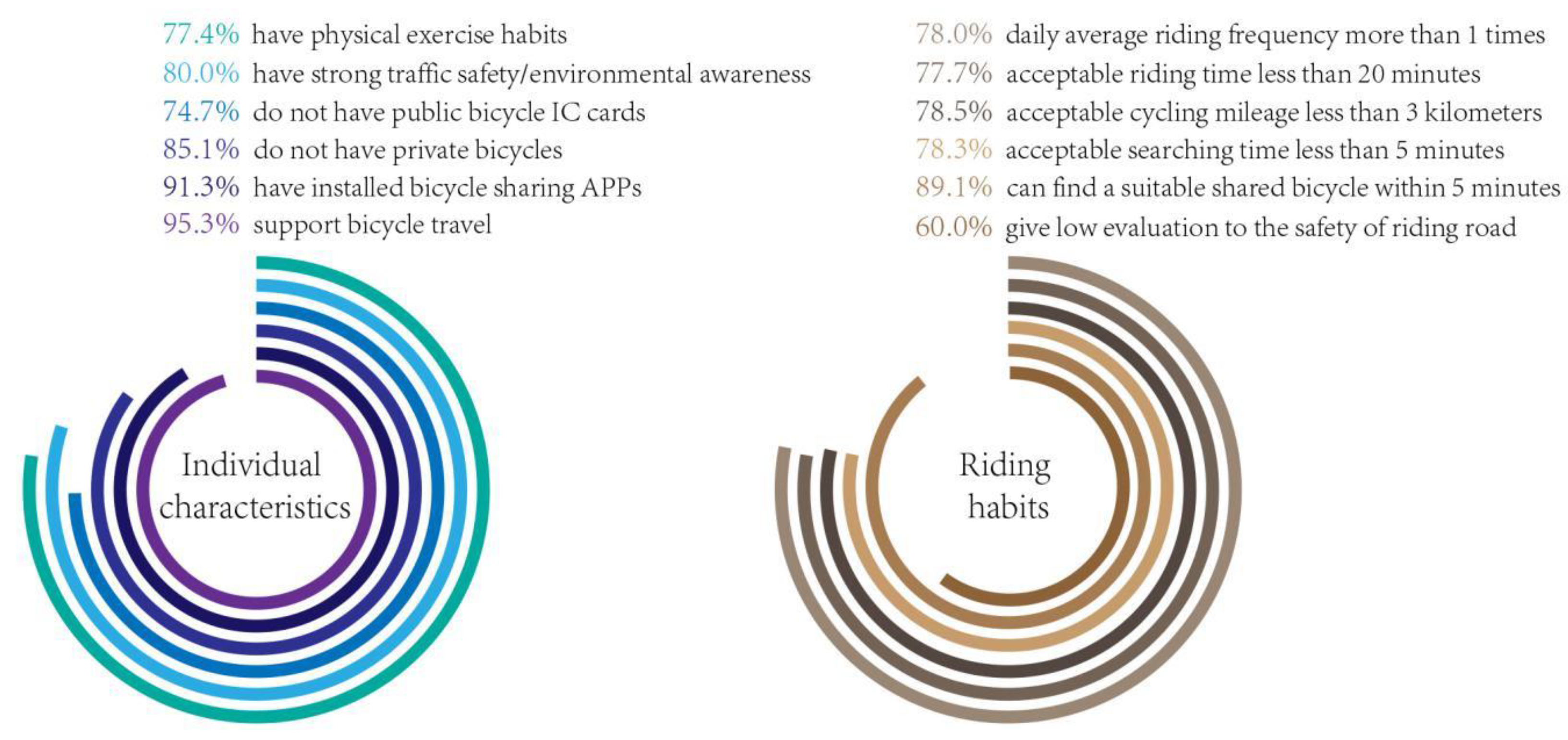
2.1.1. Individual Characteristics and Riding Habits
2.1.2. Trip Characteristics
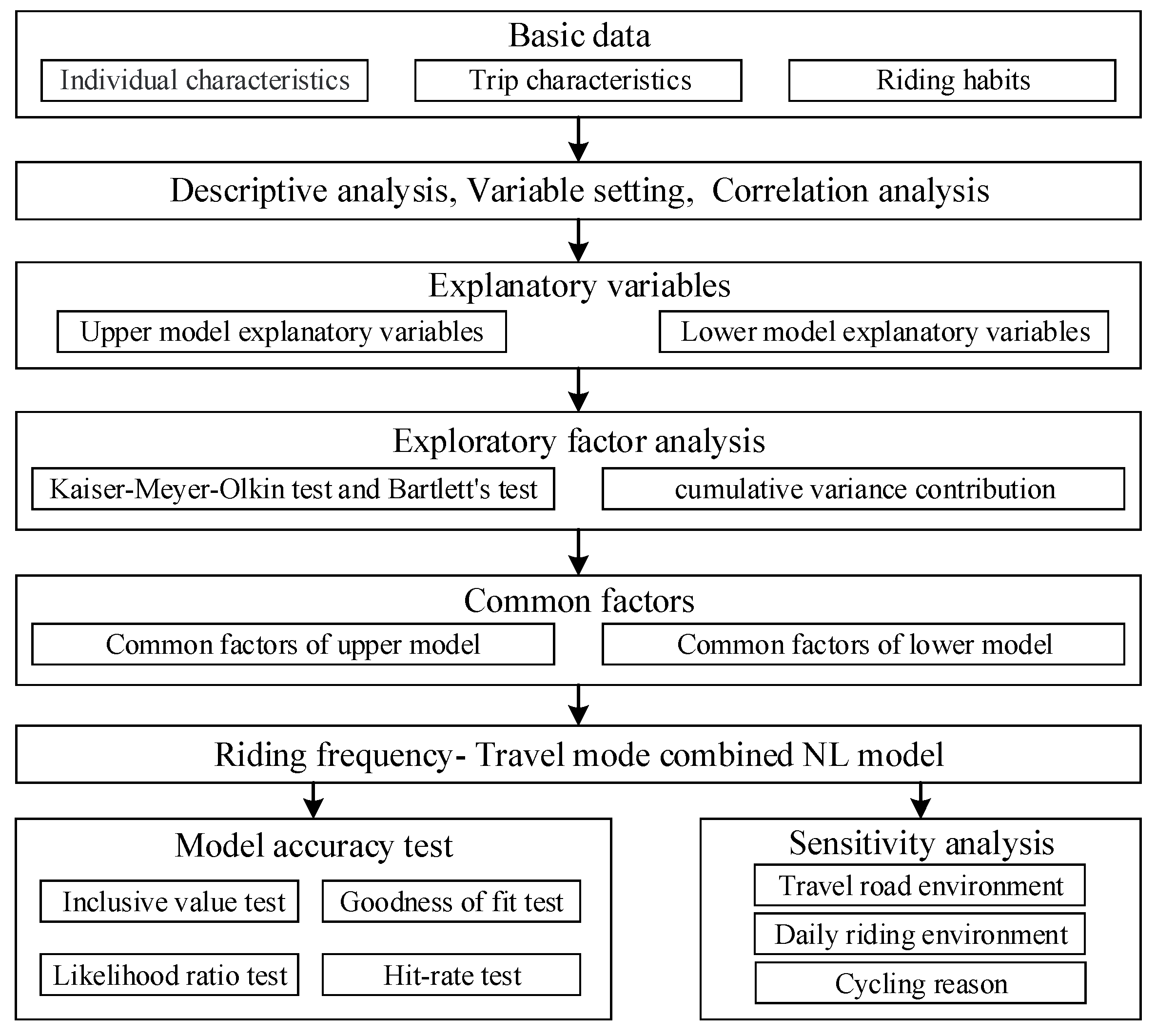
2.2. Methods
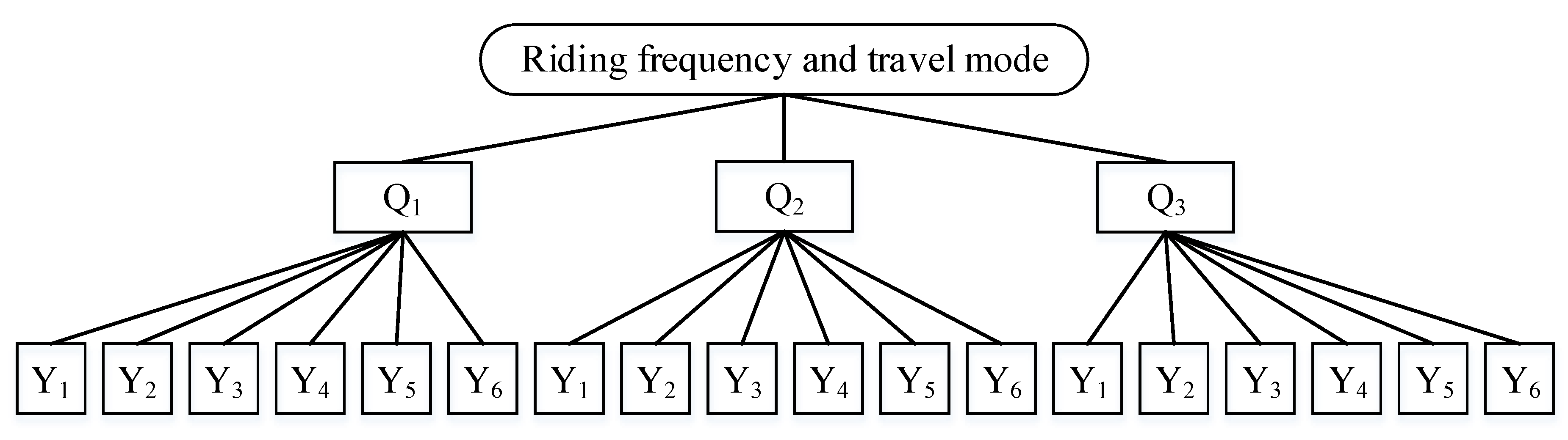
2.2.1. Nested Logit Model
2.2.2. Factor Analysis Method
3. Results
3.1. Setting of Upper and Lower Model Explanatory Variables
3.2. Exploratory Factor Analysis of Explanatory Variables
3.3. Common Factor Redefinition
3.4. Construction of NL Model Based on Common Factors
3.4.1. Calculation Results of Lower Model
3.4.2. Calculation Results of Upper Model
3.4.3. NL Model Accuracy Test
4. Discussion and Conclusions
Author Contributions
Funding
Acknowledgments
Conflicts of Interest
Appendix A. Travel Characteristics Data

| Survey Content | Option | Sample | Percent | Survey Content | Option | Sample | Percent |
|---|---|---|---|---|---|---|---|
| Gender | Male | 305 | 63.1% | Will pay attention to environmental news/events | Yes | 357 | 73.9% |
| Female | 178 | 36.9% | No | 96 | 26.1% | ||
| Education | Undergraduate | 204 | 42.2% | Can ride bicycle | Yes | 476 | 98.6% |
| Postgraduate | 279 | 57.8% | No | 7 | 1.4% | ||
| Sports frequency | Rarely | 109 | 22.6% | Has public bicycle IC card | Yes | 122 | 25.3% |
| Occasionally | 253 | 52.4% | No | 361 | 74.7% | ||
| Often | 121 | 25.0% | Installed bicycle sharing app | Neither | 42 | 8.7% | |
| Disposable living expenses (yuan) | ≤1000 | 126 | 26.1% | Only Mobike | 239 | 31.5% | |
| 1000–1500 | 239 | 49.5% | Only ofo | 133 | 45.4% | ||
| 1500–2000 | 75 | 15.5% | Both | 70 | 14.4% | ||
| ≥2000 | 43 | 9.0% | Has personal bicycle | Yes | 72 | 14.9% | |
| Waiting for traffic lights and walking on crosswalks | Will not | 5 | 1.1% | No | 411 | 85.1% | |
| Will if police nearby | 11 | 2.2% | Cycling support level | Very unsupported | 12 | 2.4% | |
| Sometimes will | 39 | 8.2% | Unsupported | 11 | 2.2% | ||
| Will | 428 | 88.6% | Supported | 337 | 69.8% | ||
| Has environmental awareness | Yes | 446 | 92.4% | ||||
| No | 21 | 4.3% | Very supported | 123 | 25.5% | ||
| Not clear | 16 | 3.3% |
| Survey Content | Option | Sample | Percent | Survey Content | Option | Sample | Percent |
|---|---|---|---|---|---|---|---|
| Riding frequency | ≤0.5 | 106 | 22.0% | Acceptable search time (min) | 1 | 27 | 5.7% |
| 1 | 222 | 45.9% | 2 | 42 | 8.7% | ||
| ≥2 | 155 | 32.1% | 3 | 60 | 12.4% | ||
| Riding time/period | Only day | 182 | 37.7% | 5 | 249 | 51.5% | |
| Only night | 7 | 1.4% | 10 | 90 | 18.7% | ||
| Day and night | 294 | 60.9% | >10 | 15 | 3% | ||
| Acceptable riding time (min) | ≤10 | 42 | 8.7% | Road safety evaluation | Very low | 41 | 8.5% |
| ≤15 | 190 | 39.4% | Low | 249 | 51.5% | ||
| ≤20 | 143 | 29.6% | High | 181 | 37.5% | ||
| >20 | 108 | 22.3% | Very high | 12 | 2.5% | ||
| Acceptable cycling distance (km) | 1 | 26 | 5.3% | Satisfaction of riding environment (scores) | 0, 1, 2 | 31 | 6.4% |
| 2 | 180 | 37.3% | 3 | 39 | 8.1% | ||
| 3 | 173 | 35.9% | 4 | 52 | 10.7% | ||
| >3 | 104 | 21.5% | 5 | 83 | 17.2% | ||
| Search time before riding (min) | 1 | 66 | 13.6% | 6 | 79 | 16.4% | |
| 2 | 121 | 25.0% | 7 | 82 | 17.0% | ||
| 3 | 98 | 20.3% | 8 | 68 | 14.0% | ||
| 5 | 146 | 30.4% | 9, 10 | 49 | 10.2% | ||
| 10 | 45 | 9.5% | |||||
| >10 | 7 | 1.4% |
Appendix B. Correlation Test Results
| Variable Category | Original Influence Factor (Code) | Type | Spearman Coefficient | Sig. | Variable Category | Original Influence Factor (Code) | Type | Spearman Coefficient | Sig. |
|---|---|---|---|---|---|---|---|---|---|
| (1) Personal features and travel mode | |||||||||
| Gender | Male (Z1) | 0–1 | 0.091 * | 0.039 | Education | Undergraduate (Z3) | 0–1 | 0.098 * | 0.026 |
| Female (Z2) | 0–1 | −0.091 * | 0.039 | Postgraduate (Z4) | 0–1 | 0.098 * | 0.026 | ||
| Environmental awareness | Will pay attention to environmental news or not (Z5) | 0–1 | 0.141 ** | 0.001 | Riding frequency | Daily riding frequency (Z6) | Continuous | 0.114 ** | 0.010 |
| (2) Riding habits and travel mode | |||||||||
| Cycling expectations | Acceptable cycling distance < 2 km (Z8) | 0–1 | 0.051 * | 0.046 | Cycling reasons | Cheap (Z22) | 0–1 | −0.092 * | 0.036 |
| Acceptable cycling distance < 3 km (Z9) | 0–1 | 0.117 * | 0.010 | Flexible (Z23) | 0–1 | −0.077 | 0.036 | ||
| Acceptable cycling distance > 3 km (Z10) | 0–1 | 0.112 * | 0.030 | Low carbon (Z24) | 0–1 | 0.128 ** | 0.003 | ||
| Acceptable riding time (Z11) | Ordered | −0.0109 * | 0.013 | Avoid traffic congestion (Z25) | 0–1 | 0.093 * | 0.035 | ||
| Acceptable searching time (Z12) | Ordered | −0.110 * | 0.012 | Lack of transport (Z26) | 0–1 | 0.115 * | 0.017 | ||
| Cycling experiences | Road safety evaluation (Z7) | Ordered | 0.111 * | 0.012 | Cycling season | Summer only (Z27) | 0–1 | −0.106 * | 0.016 |
| Operational convenience (Z13) | Ordered | −0.110 * | 0.012 | Autumn only (Z28) | 0–1 | −0.094 * | 0.033 | ||
| Searching convenience (Z14) | Ordered | −0.164 ** | 0.000 | Except winter (Z29) | 0–1 | −0.176 ** | 0.000 | ||
| Returning convenience (Z15) | Ordered | −0.096 * | 0.028 | All seasons (Z30) | 0–1 | 0.248 ** | 0.000 | ||
| Bicycle quality scores (Z16) | Ordered | −0.208 ** | 0.000 | Daily riding time | Only day (Z31) | 0–1 | −0.165 ** | 0.000 | |
| Deposit security scores (Z17) | Ordered | −0.152 ** | 0.001 | Day and night (Z32) | 0–1 | 0.169 ** | 0.000 | ||
| Riding promotion scores (Z18) | Ordered | −0.137 ** | 0.002 | Daily riding environment | Isolated bicycle lane (Z33) | 0–1 | 0.093 * | 0.035 | |
| Overall satisfaction scores (Z19) | Ordered | −0.171 ** | 0.000 | Signal lights at intersections (Z34) | 0–1 | −0.119 ** | 0.007 | ||
| Traveling purpose | Attending class (Z20) | 0–1 | −0.136 ** | 0.002 | Flat road (Z35) | 0–1 | 0.042 * | 0.038 | |
| Transferring (Z21) | 0–1 | 0.099 * | 0.025 | Campus interior (Z36) | 0–1 | −0.115 ** | 0.009 | ||
| Many pedestrians (Z37) | 0–1 | −0.103 * | 0.014 | ||||||
| (3) Trip information and travel mode | |||||||||
| Traveling characteristics | Entertainment (Z38) | 0–1 | −0.149 ** | 0.001 | Traveling road environment | Bicycle lanes (Z48) | 0–1 | 0.107 * | 0.015 |
| Shopping (Z39) | 0–1 | 0.105 * | 0.044 | Road congestion (Z49) | 0–1 | 0.463 ** | 0.000 | ||
| Returning (Z40) | 0–1 | −0.082 * | 0.031 | Many cars (Z50) | 0–1 | 0.428 ** | 0.000 | ||
| Visiting friends (Z41) | 0–1 | 0.098 * | 0.026 | Many pedestrians (Z51) | 0–1 | 0.106 * | 0.016 | ||
| Laboratory attendance (Z42) | 0–1 | 0.174 ** | 0.000 | Many intersections (Z52) | 0–1 | 0.237 ** | 0.000 | ||
| Travel time (min) (Z43) | Continuous | 0.229 ** | 0.000 | Flat road (Z53) | 0–1 | 0.098 * | 0.027 | ||
| Travel distance (km) (Z44) | Continuous | 0.533 ** | 0.000 | Through pedestrian bridge (Z54) | 0–1 | 0.117 ** | 0.008 | ||
| Traveling natural environment | Cloudy (Z45) | 0–1 | 0.180 ** | 0.000 | Complete and clear markings and signs (Z55) | 0–1 | 0.376 ** | 0.000 | |
| Sunny (Z46) | 0–1 | −0.169 ** | 0.000 | Trips on campus (Z56) | 0–1 | −0.121 ** | 0.006 | ||
| Perceived temperature (Z47) | 0–1 | −0.116 ** | 0.008 | ||||||
| Variable Category | Original Influence Factor (Influence Factor Code) | Type | Spearman Coefficient | Sig. | Variable Category | Original Influence Factor | Type | Spearman Coefficient | Sig. |
|---|---|---|---|---|---|---|---|---|---|
| (1) Personal features and riding frequency | |||||||||
| Gender | Male (M1) | 0–1 | 0.183 ** | 0.000 | Disposable living expenses | 1000–1500 (yuan) (M11) | 0–1 | −0.142 ** | 0.001 |
| Female (M2) | 0–1 | −0.183 ** | 0.000 | 1500–2000 (yuan) (M12) | 0–1 | 0.147 ** | 0.001 | ||
| Sports frequency | Rarely (M3) | 0–1 | −0.116 ** | 0.009 | IC card | Has bus IC card (M6) | 0–1 | 0.146 ** | 0.001 |
| Occasionally (M4) | 0–1 | 0.106 * | 0.016 | Bicycle usage | As major travel mode (M7) | 0–1 | 0.426 ** | 0.000 | |
| Installed bicycle sharing app | Neither (M8) | 0–1 | 0.089 * | 0.043 | Environmental awareness | Will pay attention to environmental news or not (M5) | 0–1 | 0.115 ** | 0.009 |
| Only ofo (M9) | 0–1 | 0.125 ** | 0.005 | ||||||
| Both (M10) | 0–1 | −0.208 ** | 0.000 | ||||||
| (2) Riding habits and riding frequency | |||||||||
| Daily riding time | Only day (M13) | 0–1 | −0.293 ** | 0.000 | Cycling reasons | Cheap (M25) | 0–1 | 0.192 ** | 0.000 |
| Day and night (M14) | 0–1 | 0.299 ** | 0.000 | Habit (M26) | 0–1 | 0.173 ** | 0.000 | ||
| Cycling expectations | Acceptable riding time (M15) | Ordered | 0.123 ** | 0.005 | Low carbon (M27) | 0–1 | 0.199 ** | 0.000 | |
| Acceptable searching time (M16) | Ordered | 0.132 ** | 0.003 | Avoid traffic congestion (M28) | 0–1 | 0.125 ** | 0.005 | ||
| Cycling season | Summer only (M17) | 0–1 | −0.135 ** | 0.002 | For exercise (M29) | 0–1 | 0.088 * | 0.046 | |
| All seasons (M18) | 0–1 | 0.120 ** | 0.007 | Daily riding environment | Isolated bicycle lane (M30) | 0–1 | 0.091 * | 0.040 | |
| Spring and autumn (M19) | 0–1 | −0.131 ** | 0.003 | Mixed traffic (M31) | 0–1 | −0.096 * | 0.030 | ||
| Travel purpose | Attending class (M20) | 0–1 | 0.297 ** | 0.000 | Signal lights at intersections (M32) | 0–1 | 0.134 ** | 0.002 | |
| Shopping (M21) | 0–1 | 0.112 * | 0.011 | Not pass pedestrian bridge (M33) | 0–1 | 0.106 * | 0.016 | ||
| Daily bicycle riding | Public bicycle (M22) | 0–1 | 0.155 ** | 0.000 | Campus interior (M34) | 0–1 | 0.093 * | 0.036 | |
| Mobike (M23) | 0–1 | 0.110 * | 0.012 | Traveling road environment | Road congestion (M35) | 0–1 | 0.161 ** | 0.000 | |
| ofo (M24) | 0–1 | −0.092 * | 0.038 | Trips on campus (M36) | 0–1 | 0.114 ** | 0.010 | ||
| Lower Model | |||
|---|---|---|---|
| Common Factor Code | Renamed Common Factor | Expression | Cronbach α Reliability Coefficient |
| x1 | Cycling experiences factor | x1 = 0.207Z13 + 0.201Z14 + 0.207Z15 + 0.160Z16 + 0.173Z17 + 0.182Z18 + 0.208Z19 | 0.857 |
| x2 | Traveling road environment factor 1 | x2 = 0.173Z48 + 0.262Z51 + 0.215Z52 − 0.309Z56 | 0.704 |
| x3 | Traveling road environment factor 2 | x3 = 0.234Z39 + 0.253Z50 + 0.240Z53 − 0.270Z54 + 0.232Z55 | 0.748 |
| x4 | Traveling characteristics factor | x4 = 0.296Z43 + 0.348Z44 + 0.208Z49 | 0.801 |
| x5 | Daily riding time factor 1 | x5 = −0.401Z31 + 0.412Z32 | 0.823 |
| x6 | Gender factor 1 | x6 = 0.475Z1 − 0.475Z2 | 0.743 |
| x7 | Education factor 1 | x7 = −0.389Z3 + 0.389Z4 | 0.798 |
| x8 | Cycling expectation factor 1 | x8 = 0.465Z10 + 0.446Z11 | 0.720 |
| x9 | Traveling natural environment factor | x9 = 0.404Z45 − 0.399Z46 − 0.35Z47 | 0.827 |
| x10 | Cycling expectation factor 2 | x10 = −0.463Z8 + 0.520Z9 | 0.767 |
| x11 | Cycling season factor 1 | x11 = −0.464Z29 + 0.369Z30 | 0.832 |
| x12 | Comprehensive factor 1 | x12 = 0.416Z21 + 0.266Z24 − 0.418Z26 − 0.141Z28 + 0.204Z33 | 0.661 |
| x13 | Comprehensive factor 2 | x13 = 0.449Z6 + 0.297Z20 | 0.773 |
| x14 | Daily riding environment factor 1 | x14 = 0.331Z25 + 0.436Z34 + 0.274Z35 | 0.804 |
| x15 | Comprehensive factor 3 | x15 = 0.269Z5 − 0.468Z37 + 0.404Z42 | 0.693 |
| x16 | Traveling purpose factor 1 | x16 = 0.434Z38 − 0.56Z40 | 0.819 |
| x17 | Cycling season factor 2 | x17 = 0.541Z27 | -- |
| x18 | Comprehensive factor 4 | x18 = 0.327Z7 + 0.191Z12 + 0.502Z23 | 0.732 |
| x19 | Traveling purpose factor 2 | x19 = −0.566Z41 | -- |
| Upper model | |||
| w1 | Daily riding time factor 2 | w1 = −0.399M13 + 0.399M14 | 0.823 |
| w2 | Gender factor 2 | w2 = 0.445M1 − 0.445M2 | 0.743 |
| w3 | Comprehensive factor 5 | w3 = −0.493M8 − 0.445M24 | 0.657 |
| w4 | Comprehensive factor 6 | w4 = 0.511M9 + 0.462M23 | 0.710 |
| w5 | Education factor 2 | w5 = 0.511M3 − 0.547M4 | 0.798 |
| w6 | Disposable living expenses factor | w6 = −0.561M11 + 0.531M12 | 0.836 |
| w7 | Comprehensive factor 7 | w7 = 0.205M7 + 0.427M21 + 0.428M29 | 0.749 |
| w8 | Daily riding environment factor 2 | w8 = 0.554M34 + 0.503M36 | 0.715 |
| w9 | Comprehensive factor 8 | w9 = 0.272M18 − 0.364M19 + 0.365M25 + 0.44M30 | 0.802 |
| w10 | Comprehensive factor 9 | w10 = −0.329M10 − 0.547M17 + 0.267M20 | 0.735 |
| w11 | Comprehensive factor 10 | w11 = 0.351M5 − 0.339M26 + 0.411M32 + 0.353M35 | 0.651 |
| w12 | Public bicycle factor | w12 = 0.376M6 + 0.497M22 | 0.809 |
| w13 | Cycling reasons factor | w13 = 0.613M27 + 0.210M28 | 0.763 |
| w14 | Cycling expectation factor 3 | w14 = 0.574M15 + 0.506M16 | 0.776 |
| w15 | Daily riding environment factor 3 | w15 = −0.507M31 + 0.632M33 | 0.808 |
References
- Home, S. The Assault on Culture Utopian Currents from Lettrisme to Class War. J. Elect. Soc. 1991, 153, 713–718. [Google Scholar]
- Bachand-Marleau, J.; Lee, B.H.Y.; El-Geneidy, A.M. Better Understanding of Factors Influencing Likelihood of Using Shared Bicycle Systems and Frequency of Use. Transp. Res. Rec. J. Transp. Res. Board 2012, 2314, 66–71. [Google Scholar] [CrossRef]
- Behrendt, F. Why cycling matters for Smart Cities. Internet of Bicycles for Intelligent Transport. J. Transp. Geogr. 2016, 56, 157–164. [Google Scholar] [CrossRef]
- DeMaio, P. Smart bikes: Public transportation for the 21st century. Transp. Q. 2003, 57, 9–11. [Google Scholar]
- DeMaio, P.; Gifford, J. Will Smart Bikes Succeed as Public Transportation in the United States? J. Public Transp. 2004, 7, 1–15. [Google Scholar] [CrossRef]
- Tang, Y.; Pan, H.; Fei, Y. Research on Users’ Frequency of Ride in Shanghai Minhang Bike-sharing System. Transp. Res. Procedia 2017, 25, 4979–4987. [Google Scholar] [CrossRef]
- Wuhan Institute of Transportation Development Strategy. 2017 Wuhan City Shared Bicycle Travel Report; Wuhan Transportation Development Strategy Research Institute: Wuhan, China, 2017. [Google Scholar]
- Handy, S.L.; Xing, Y.; Buehler, T.J. Factors associated with bicycle ownership and use: A study of six small U.S. cities. Transportation 2010, 37, 967–985. [Google Scholar] [CrossRef]
- Li, Z.; Wang, W.; Yang, C.; Jiang, G. Exploring the causal relationship between bicycle choice and trip chain pattern. Transp. Policy 2013, 29, 170–177. [Google Scholar] [CrossRef]
- Nankervis, M. The effect of weather and climate on bicycle commuting. Transp. Res. Part A Policy Pract. 1999, 33, 417–431. [Google Scholar] [CrossRef]
- Stinson, M.A.; Bhat, C.R.; Information, R. Commuter Bicyclist Route Choice: Analysis Using a Stated Preference Survey. Transp. Res. Rec. J. Transp. Res. Board 2003, 1828, 107–115. [Google Scholar] [CrossRef]
- Campbell, A.A.; Cherry, C.R.; Ryerson, M.S.; Yang, X. Factors influencing the choice of shared bicycles and shared electric bikes in Beijing. Transp. Res. Part C Emerg. Technol. 2016, 67, 399–414. [Google Scholar] [CrossRef]
- Dickinson, J.E.; Kingham, S.; Copsey, S.; Hougie, D.J. Employer travel plans, cycling and gender: Will travel plan measures improve the outlook for cycling to work in the UK? Transp. Res. Part D Transp. Environ. 2003, 8, 53–67. [Google Scholar] [CrossRef]
- Mohanty, S.; Blanchard, S. Complete Transit: Evaluating Walking and Biking to Transit Using a Mixed Logit Mode Choice Model. In Proceedings of the 95th Transportation Research Board Annual Meeting, Washington, DC, USA, 10–14 January 2016. [Google Scholar]
- Moudon, A.V.; Lee, C.; Cheadle, A.D.; Collier, C.W.; Johnson, D.; Schmid, T.L.; Weather, R.D. Cycling and the built environment, a US perspective. Transp. Res. Part D Transp. Environ. 2005, 10, 245–261. [Google Scholar] [CrossRef]
- Li, Z.; Wang, W.; Yang, C. Interrelationship and Order of Decision between Bicycle Choice and Trip Chain Pattern. In Proceedings of the 92th Transportation Research Board Annual Meeting, Washington, DC, USA, 13–17 January 2013. [Google Scholar]
- Ding, C.; Mishra, S.; Lin, Y. Cross-Nested Joint Model of Travel Mode and Departure Time Choice for Urban Commuting Trips: Case Study in aryland- Washington, DC Region. J. Urban Plan. Dev. 2014, 141. [Google Scholar] [CrossRef]
- De Jong, G.; Daly, A.; Pieters, M.; Vellay, C.; Bradley, M.; Hofman, F. A model for time of day and mode choice using error components logit. Transp. Res. Part E Logist. Transp. Rev. 2003, 39, 245–268. [Google Scholar] [CrossRef]
- Faghih-Imani, A.; Hampshire, R.; Marla, L.; Eluru, N. An empirical analysis of bike sharing usage and rebalancing: Evidence from Barcelona and Seville. Transp. Res. Part A Policy Pract. 2017, 97, 177–191. [Google Scholar] [CrossRef]
- Hess, D.B. Effect of Free Parking on Commuter Mode Choice: Evidence from Travel Diary Data. Transp. Res. Rec. J. Transp. Res. Board 2001, 1753, 35–42. [Google Scholar] [CrossRef]
- Mitra, R.; Buliung, R.N.; Roorda, M.J. The Built Environment and School Travel Mode Choice in Toronto. Transp. Res. Rec. 2010, 2156, 150–159. [Google Scholar] [CrossRef]
- Guo, Y.; Zhou, J.; Wu, Y.; Li, Z. Identifying the factors affecting bike-sharing usage and degree of satisfaction in Ningbo, China. PLoS ONE 2017, 12, e0185100. [Google Scholar] [CrossRef]
- Davidov, E. Explaining Habits in a New Context the Case of Travel-Mode Choice. Ration. Soc. 2007, 19, 315–334. [Google Scholar] [CrossRef]
- Yu, Z.L. Analysis and Modeling of College Students’ Travel Behavior under the Influence of Shared Bicycles. Ph.D. Thesis, Chang’an Univeisity, Xi’an, China, 2018. [Google Scholar]
- Yang, L.; Shao, C.; Haghani, A. Nested logit model of combined selection for travel mode and departure time. J. Traf. Transp. 2012, 12, 76–83. [Google Scholar]


| Survey Content | Option | Sample | Percent | Survey Content | Option | Sample | Percent |
|---|---|---|---|---|---|---|---|
| Travel mode | Walking | 232 | 48% | Travel purpose | Attending class | 135 | 28% |
| ofo | 125 | 26% | Returning | 112 | 23% | ||
| Mobike | 63 | 13% | Shopping | 72 | 15% | ||
| Transit | 24 | 5% | Entertainment | 72 | 15% | ||
| Subway | 24 | 5% | Lab attendance | 53 | 11% | ||
| Public bicycle | 10 | 2% | Transferring | 24 | 5% | ||
| Personal bicycle | 0 | 0% | Visiting friends | 15 | 3% | ||
| Taxi | 5 | 1% | |||||
| Travel distance (km) | ≤0.5 | 59 | 12.2% | Travel time (min) | ≤5 | 42 | 8.7% |
| 0.5–1 | 65 | 13.4% | 5–10 | 156 | 32.3% | ||
| 1–1.5 | 197 | 41.0% | 10–15 | 122 | 25.3% | ||
| 1.5–2 | 96 | 19.8% | 15–20 | 97 | 20.1% | ||
| 2–4 | 33 | 6.8% | 20–25 | 46 | 9.5% | ||
| >4 | 33 | 6.8% | >25 | 20 | 4.1% |
| Variables | (Z13) | (Z14) | (Z15) | (Z16) | (Z17) | (Z18) | (Z19) | |
|---|---|---|---|---|---|---|---|---|
| Operational convenience (Z13) | Pearson | 1.000 | 0.335 | 0.316 | 0.264 | 0.241 | 0.229 | 0.382 |
| Sig. | 0.000 | 0.000 | 0.000 | 0.000 | 0.000 | 0.000 | ||
| Searching convenience (Z14) | Pearson | 0.335 | 1.000 | 0.335 | 0.314 | 0.215 | 0.185 | 0.480 |
| Sig. | 0.000 | 0.000 | 0.000 | 0.000 | 0.001 | 0.000 | ||
| Returning convenience (Z15) | Pearson | 0.316 | 0.335 | 1.000 | 0.233 | 0.210 | 0.187 | 0.391 |
| Sig. | 0.000 | 0.000 | 0.000 | 0.000 | 0.001 | 0.000 | ||
| Bicycle quality scores (Z16) | Pearson | 0.264 | 0.314 | 0.233 | 1.000 | 0.343 | 0.229 | 0.421 |
| Sig. | 0.000 | 0.000 | 0.000 | 0.000 | 0.000 | 0.000 | ||
| Deposit security scores (Z17) | Pearson | 0.241 | 0.215 | 0.210 | 0.343 | 1.000 | 0.301 | 0.431 |
| Sig. | 0.000 | 0.000 | 0.000 | 0.000 | 0.000 | 0.000 | ||
| Riding promotion scores (Z18) | Pearson | 0.229 | 0.185 | 0.187 | 0.229 | 0.301 | 1.000 | 0.270 |
| Sig. | 0.000 | 0.001 | 0.001 | 0.000 | 0.000 | 0.000 | ||
| Overall satisfaction scores (Z19) | Pearson | 0.382 | 0.480 | 0.391 | 0.421 | 0.431 | 0.270 | 1.000 |
| Sig. | 0.000 | 0.000 | 0.000 | 0.000 | 0.000 | 0.000 | ||
| Component | Initial Eigenvalues | Extraction Sums of Squared Loadings | Rotation Sums of Squared Loadings | ||||||
|---|---|---|---|---|---|---|---|---|---|
| Eigenvalue | % of Variance | Total % Variance | Eigenvalue | % of Variance | Total % Variance | Eigenvalue | % of Variance | Total % Variance | |
| Lower Level | |||||||||
| 1 | 5.05 | 9.02 | 9.02 | 5.05 | 9.02 | 9.02 | 4.03 | 7.21 | 7.21 |
| 2 | 3.86 | 6.90 | 15.92 | 3.86 | 6.90 | 15.92 | 3.30 | 5.89 | 13.10 |
| 19 | 1.04 | 1.88 | 69.43 | 1.04 | 1.86 | 69.43 | 1.22 | 2.18 | 69.43 |
| 20 | 0.99 | 1.77 | 71.20 | ||||||
| 56 | 0 | 0 | 100 | ||||||
| Upper Level | |||||||||
| 1 | 3.54 | 9.83 | 9.83 | 3.54 | 9.83 | 9.83 | 2.46 | 6.84 | 6.84 |
| 2 | 2.35 | 6.54 | 16.38 | 2.35 | 6.54 | 16.38 | 2.36 | 6.55 | 13.40 |
| 15 | 1.02 | 2.85 | 68.43 | 1.02 | 2.85 | 68.43 | 1.25 | 3.47 | 68.43 |
| 16 | 0.95 | 2.64 | 71.07 | ||||||
| 36 | 0.78 | 2.17 | 80.60 | ||||||
| Factor | Score | Factor | Score | Factor | Score | Factor | Score | Factor | Score | Factor | Score |
|---|---|---|---|---|---|---|---|---|---|---|---|
| Z1 | 0.009 | Z11 | 0.004 | Z21 | −0.005 | Z31 | 0.007 | Z41 | −0.001 | Z51 | 0.007 |
| Z2 | −0.009 | Z12 | −0.008 | Z22 | −0.003 | Z32 | −0.008 | Z42 | −0.001 | Z52 | 0.005 |
| Z3 | 0.005 | Z13 | 0.207 | Z23 | −0.007 | Z33 | 0.008 | Z43 | 0.008 | Z53 | −0.009 |
| Z4 | −0.005 | Z14 | 0.201 | Z24 | −0.005 | Z34 | −0.002 | Z44 | 0.006 | Z54 | 0.002 |
| Z5 | −0.003 | Z15 | 0.207 | Z25 | −0.004 | Z35 | −0.003 | Z45 | 0.004 | Z55 | 0.002 |
| Z6 | −0.004 | Z16 | 0.160 | Z26 | 0.000 | Z36 | 0.009 | Z46 | −0.010 | Z56 | −0.009 |
| Z7 | 0.004 | Z17 | 0.173 | Z27 | −0.001 | Z37 | −0.007 | Z47 | −0.016 | ||
| Z8 | −0.005 | Z18 | 0.182 | Z28 | 0.006 | Z38 | −0.006 | Z48 | 0.008 | ||
| Z9 | 0.006 | Z19 | 0.208 | Z29 | 0.003 | Z39 | 0.002 | Z49 | 0.001 | ||
| Z10 | −0.008 | Z20 | 0.001 | Z30 | 0.004 | Z40 | −0.005 | Z50 | 0.001 |
| Travel Mode | Explanatory Variables | Coefficient | Standard Error | Wald Value | df | Significance |
|---|---|---|---|---|---|---|
| Walking | Constant | 7.521 | 5.574 | 7.282 | 1 | 0.007 |
| x1 | 3.061 | 2.567 | 5.687 | 1 | 0.017 | |
| x2 | 1.586 | 1.609 | 3.884 | 1 | 0.049 | |
| x3 | −1.948 | 1.235 | 9.954 | 1 | 0.002 | |
| x5 | 1.109 | 1.023 | 4.697 | 1 | 0.030 | |
| x7 | −2.391 | 1.998 | 5.599 | 1 | 0.018 | |
| x9 | −1.748 | 1.545 | 5.119 | 1 | 0.024 | |
| Public bicycle | x1 | −1.080 | 2.756 | 5.532 | 1 | 0.019 |
| x3 | 0.776 | 1.580 | 8.680 | 1 | 0.003 | |
| x12 | −0.631 | 1.870 | 4.098 | 1 | 0.043 | |
| Mobike | Constant | 3.420 | 5.575 | 6.020 | 1 | 0.014 |
| x1 | 1.445 | 2.569 | 5.065 | 1 | 0.024 | |
| x3 | −0.792 | 1.234 | 6.582 | 1 | 0.010 | |
| x5 | 0.538 | 1.030 | 4.367 | 1 | 0.037 | |
| x7 | −1.290 | 2.008 | 6.604 | 1 | 0.010 | |
| x9 | −0.797 | 1.549 | 4.239 | 1 | 0.040 | |
| ofo | Constant | 5.430 | 5.575 | 6.412 | 1 | 0.011 |
| x1 | 2.274 | 2.568 | 5.301 | 1 | 0.021 | |
| x3 | −1.367 | 1.237 | 8.258 | 1 | 0.004 | |
| x7 | −2.207 | 2.007 | 8.170 | 1 | 0.004 | |
| x9 | −1.270 | 1.547 | 4.558 | 1 | 0.033 | |
| Transit | x9 | −1.150 | 1.537 | 4.365 | 1 | 0.037 |
| x10 | −0.825 | 1.004 | 5.291 | 1 | 0.021 | |
| x13 | −1.045 | 1.394 | 4.404 | 1 | 0.036 | |
| x14 | 1.145 | 1.526 | 4.415 | 1 | 0.036 | |
| x19 | −1.834 | 2.033 | 6.378 | 1 | 0.012 |
| Riding Frequency (Times/Day) | Explanatory Variables | Coefficient | Standard Error | Wald Value | df | Significance |
|---|---|---|---|---|---|---|
| >0.5 to ≤1 | Constant | 1.999 | 0.484 | 17.041 | 1 | 0.000 |
| w1 | 0.808 | 0.143 | 32.023 | 1 | 0.000 | |
| w3 | 0.465 | 0.181 | 6.586 | 1 | 0.010 | |
| w4 | 0.306 | 0.142 | 4.615 | 1 | 0.032 | |
| w5 | −0.504 | 0.130 | 14.957 | 1 | 0.000 | |
| w6 | −0.338 | 0.131 | 6.600 | 1 | 0.010 | |
| w10 | 0.349 | 0.125 | 7.836 | 1 | 0.005 | |
| w13 | 0.359 | 0.142 | 6.415 | 1 | 0.011 | |
| w14 | 0.430 | 0.156 | 7.539 | 1 | 0.006 | |
| w15 | 0.384 | 0.158 | 5.910 | 1 | 0.015 | |
| Logsum (1/μ) | 0.251 | 0.166 | 8.437 | 1 | 0.000 | |
| >1 | Constant | 1.691 | 0.538 | 9.889 | 1 | 0.002 |
| w1 | 1.038 | 0.168 | 38.159 | 1 | 0.000 | |
| w2 | 0.575 | 0.161 | 12.726 | 1 | 0.000 | |
| w3 | 0.762 | 0.196 | 15.178 | 1 | 0.000 | |
| w4 | 0.433 | 0.161 | 7.284 | 1 | 0.007 | |
| w5 | −0.611 | 0.154 | 15.815 | 1 | 0.000 | |
| w6 | −0.598 | 0.161 | 13.868 | 1 | 0.000 | |
| w7 | 0.643 | 0.156 | 16.979 | 1 | 0.000 | |
| w8 | 0.377 | 0.160 | 5.583 | 1 | 0.018 | |
| w9 | 0.333 | 0.166 | 4.044 | 1 | 0.044 | |
| w10 | 0.689 | 0.164 | 17.746 | 1 | 0.000 | |
| w11 | 0.641 | 0.183 | 12.253 | 1 | 0.000 | |
| w13 | 0.406 | 0.161 | 6.361 | 1 | 0.012 | |
| w14 | 0.616 | 0.173 | 12.675 | 1 | 0.000 | |
| w15 | 0.652 | 0.175 | 13.925 | 1 | 0.000 | |
| Logsum (1/μ) | 0.373 | 0.165 | 6.682 | 1 | 0.001 |
| Lower Model | |||||||||||
| Travel Mode | Prediction Results | ||||||||||
| Walking | Public Bicycle | Mobike | ofo | Transit | Subway | Total | |||||
| Actual choice | Walking | 211 (85.4%) | 4 | 6 | 14 | 2 | 0 | 237 | |||
| Public bicycle | 1 | 7 (58.3%) | 0 | 1 | 0 | 0 | 13 | ||||
| Mobike | 8 | 0 | 51 (72.9%) | 2 | 0 | 0 | 61 | ||||
| ofo | 24 | 1 | 12 | 117 (86.0%) | 1 | 0 | 138 | ||||
| Transit | 2 | 0 | 1 | 1 | 21 (84.0%) | 1 | 26 | ||||
| Subway | 1 | 0 | 0 | 1 | 1 | 26 (96.3%) | 29 | ||||
| Total | 247 | 12 | 70 | 136 | 25 | 27 | 517 (83.7%) | ||||
| Upper model | |||||||||||
| Riding frequency | Prediction results | ||||||||||
| ≤0.5 | 0.5–1 | >1 | Total | ||||||||
| Actual choice | ≤0.5 | 82 (82%) | 9 | 7 | 98 | ||||||
| 0.5–1 | 15 | 185 (78.39%) | 44 | 244 | |||||||
| >1 | 3 | 42 | 130 (71.82%) | 175 | |||||||
| Total | 100 | 236 | 181 | 517 (76.8%) | |||||||
© 2019 by the authors. Licensee MDPI, Basel, Switzerland. This article is an open access article distributed under the terms and conditions of the Creative Commons Attribution (CC BY) license (http://creativecommons.org/licenses/by/4.0/).
Share and Cite
Ma, S.; Zhou, Y.; Yu, Z.; Zhang, Y. College Students’ Shared Bicycle Use Behavior Based on the NL Model and Factor Analysis. Sustainability 2019, 11, 4538. https://doi.org/10.3390/su11174538
Ma S, Zhou Y, Yu Z, Zhang Y. College Students’ Shared Bicycle Use Behavior Based on the NL Model and Factor Analysis. Sustainability. 2019; 11(17):4538. https://doi.org/10.3390/su11174538
Chicago/Turabian StyleMa, Shuhong, Yechao Zhou, Zhoulin Yu, and Yan Zhang. 2019. "College Students’ Shared Bicycle Use Behavior Based on the NL Model and Factor Analysis" Sustainability 11, no. 17: 4538. https://doi.org/10.3390/su11174538
APA StyleMa, S., Zhou, Y., Yu, Z., & Zhang, Y. (2019). College Students’ Shared Bicycle Use Behavior Based on the NL Model and Factor Analysis. Sustainability, 11(17), 4538. https://doi.org/10.3390/su11174538