Regional Differences in Municipal Solid Waste Collection Quantities in China

Abstract

The rapid growth in urban population has led to a dramatic increase in municipal solid waste (MSW) generation, with ramifications more pronounced in developing countries. The regional Chinese governments have made great efforts to reduce MSW generation and collection quantities. However, the results of these efforts vary across cities. The purpose of this paper is to analyze the regional differences in MSW collection quantities. A two-level hierarchical linear model (HLM) was used to examine the variations in MSW collection quantities among 287 prefecture-level cites in China over the period from 2008 to 2017. The analysis reveals a strong negative correlation between the regional economic development level and the growth trend of MSW collection quantities. The empirical findings indicate that the level of economic development and waste collection measures are critical determinants of MSW collection quantities.

1. Introduction

China is one of the largest municipal solid waste (MSW) producers in the world, generating over 150 million tons of MSW per year, accounting for 29% of the world total [1]. MSW is recognized as one major problem affecting the environmental quality and sustainable development of China’s cities [2]. The local governments have dedicated efforts to tackle the MSW problem, especially on MSW collection quantities. The MSW collection quantities vary from city to city by a variety of economic, social, and cultural factors, making it difficult for a city to adopt a waste collection service that may prove to be successful in other cities. Therefore, it is necessary to investigate the regional differences in MSW collection quantities and the growth trend of MSW collection quantities.

MSW collection quantities are an important indicator of the waste collection service level and capability of a nation or a region. The quantity of MSW collection varies by several factors. Many studies have been conducted to explore the factors influencing MSW quantities, such as economic factors (gross domestic product (GDP), consumption expenditure, income), geographical environment factors (urban scale), political factors (MSW policy regulation), social factors (culture, education, occupation), etc. [3,4,5,6,7,8,9,10]. With special regard to the influencing factors of MSW collection performance, several factors including economic, MSW collection service form, and transport routes have been studied. In particular, economic aspects are found to influence the success of implementing waste collection programs [11,12,13]. Several studies have also confirmed that the private sector or private companies provide MSW collection services more effectively than the public sector or public companies [14,15,16,17,18]. The private companies are found to use the collection crew more efficiently and set a higher demand or expectation on MSW collection [19,20,21]. Optimal MSW collection and transportation schemes (GIS, algorithm, etc.) have been proposed by scholars and applied to develop the shortest distance waste collection strategy so as to further improve waste collection efficiency [22,23,24,25,26,27]. Considering the influencing factors of both MSW quantities and collection performance together comprehensively, economic factors appear to exert significant influences on MSW collection quantities.

Observing and understanding the trend of MSW collection quantities can help policy makers develop pertinent and sustainable measures and policies of MSW collection over the long term. Trends observed regarding MSW in Japan, Copenhagen, Ontario, and the Philippines were discussed and analyzed [28,29,30,31]. Multivariate grey models, artificial intelligence models, S-curve trend models, and hidden Markov models, etc. have been used by researchers for forecasting MSW quantities [32,33,34,35,36,37,38]. The majority of previous studies mainly focus on MSW collection trends and quantity predictions. These studies often rely on case studies and small datasets, ignoring the direct interactions between MSW collection quantities and the extent and stage of economic development at a regional and national level. Both natural and economic conditions exhibit large regional differences in China [39]. The areas with different economic development levels carry out different MSW collection services, which affect the quantity of MSW collection directly. Therefore, it is necessary to analyze and conduct research on MSW collection quantities from the perspective of regional differences. Several mathematical models have been proposed to study MSW collection differences. Data envelopment analysis (DEA), a commonly used method to study MSW collection, is designed and focused on measuring the environmental efficiency in waste generation and waste service [40,41,42,43]. A practical allocation model is applicable to treat MSW [44]. For regional differences in MSW, political, economic, social, legal, technological and environmental (PESLTE) was employed to explain the differences in household food waste collection and treatment provisions between local authorities in England and Wales [45]. Regression models were applied to analyze the differences in paper waste and plastic packaging waste, respectively [46,47]. An EKC (environmental Kuznets curve) was used as an analytical framework to analyze the relation between waste generation and economic conditions [48,49,50,51]. However, these models have not seemed to be applied well to analyze the regional differences in MSW collection quantity changes over time.

There are several options for measuring changes over time, including repeated measures, hierarchical linear modeling (HLM), ANOVA, multivariate repeated measures (MRM), or structural equation models (SEM) [52,53,54,55,56,57]. Among them, repeated measures and ANOVA don’t allow for missing data in time periods, and MRM and SEW have limitations in dealing with the multilevel data [58]. Considering the inherent nature of time periods nested within regions of different economic development levels, HLM can describe the underlying structure and predictors of growth or change over time. HLM methodology has been widely used in many fields [58,59,60], and is proposed here as an appropriate multilevel tool to measure changes over time in MSW collection quantities.

There have been few studies conducted in the field of MSW collection. This paper attempts to add and contribute to the existing literature. With such an aim, the objectives of this empirical study are: (i) to confirm the relationship between regional economic development levels and MSW collection; (ii) to analyze the various reasons for regional differences in MSW collection; and (iii) to provide valuable information for MSW collection.

2. Materials and Methods

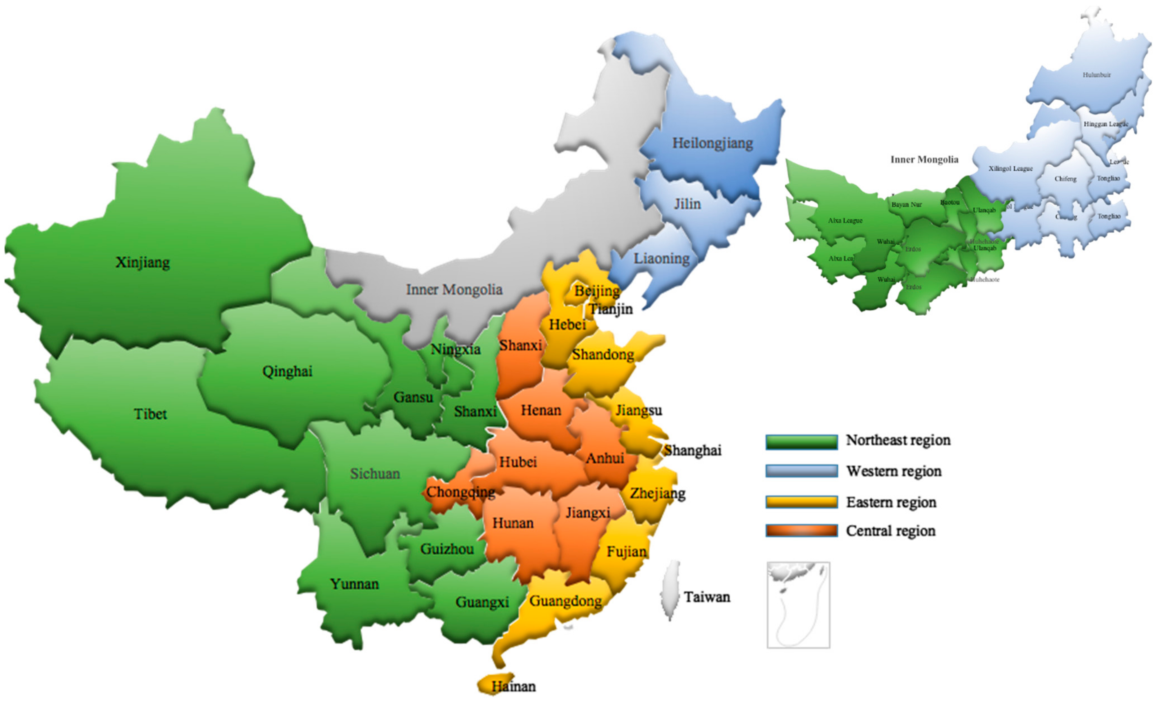
2.1. Study Location

China is divided into four major economic regions by the authorities according to the “Opinions of the Central Committee of the Communist Party of China and the State Council on Promoting the Rise of the Central Region”, the “Implementation Opinions of the State Council on Several Policy Measures for the Development of the Western Region”, and the spirit of the 16th National Congress of the Communist Party of China. Based on the economic development level (GDP, proportion of added value of service industry and urbanization rate of permanent residents), China can be divided into four regions: the northeast region, the central region, the eastern region, and the western region, as in Figure 1 below. The four economic regions contain 293 prefecture-level cities, in which Qamdo, Nyingchi, Shannan, Naqu, Sansha, and Haidong were established after 2011. To investigate the variations in MSW collection quantities from 2008 to 2017, we exclude these six recently established cities and focus on 287 prefecture-level cites, which were grouped into four regions: the northeast region (37 prefecture-level cities), central region (80 prefecture-level cities), eastern region, (84 prefecture-level cities), and western region (86 prefecture-level cities).

2.2. Variable Design and Hypotheses

2.2.1. The Design of the Outcome Variable and Hypothesis

The outcome variables are MSW collection quantities. The MSW collection quantities refer to the quantity that can be collected and transported to the transfer station or disposal site with exception regarding the quantity of waste transferred the second time. According to Olle Hage, many factors influence collection quantities to various degrees [47]. The quantity of waste differs significantly across different districts or counites. The municipalities that employ weight-based waste management fees generally experience higher collection rates, and better managed districts tend to collect less waste [45,61,62]. MSW collection actually varies in different ways across different cities of China. We hypothesize the following regarding the outcome variable:

Hypothesis 1.

The MSW collection quantities exhibit significant individual differences across cities.

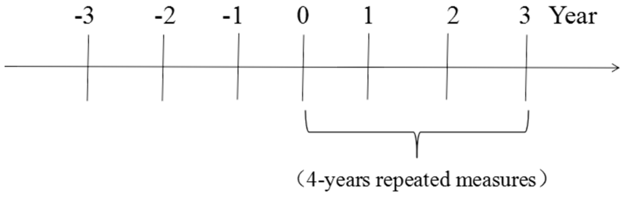
2.2.2. The Design of the Time Variable and Hypothesis

The time variable is the observation time of MSW collection quantities. The quantities of MSW change over time. The quantities of MSW have been growing rapidly in many nations or regions [34,35,36,37]. In order to better reflect the changing trend of MSW collection quantities, 10 years of historical data in MSW collection from 2008 to 2017 for 287 cities have been used, and we can hypothesize the following:

Hypothesis 2.

The MSW collection quantities are positively related to the time variable.

2.2.3. The Design of the Predictive Variables and Hypothesis

The predictive variables refer to the economic development level variables (some of them time-invariant) that can explain or characterize MSW collection quantities of regions in this study. The associations between economic conditions and waste quantities have been confirmed in previous studies [3,4,5,6,10,63,64]. Most of these research works have found a positive correlation between economic development level and MSW collection quantities. Nonetheless, since 2000, waste source classification has been adopted in the more developed regions in China [65]. The growth rate of MSW collection quantities in these cities slowed slightly. Therefore, we hypothesize the following:

Hypothesis 3.

The economic development level would be negatively related to the growth rate in MSW collection quantities over time.

Based on the variable design and hypotheses, the require data used in this study were collected by a team of student research assistants and faculty researchers from the Economics and Management School at Harbin Engineering University that have both a research background and understanding of MSW. Historical data for 287 prefecture-level cities over the period of 2008 to 2017 were obtained from the China Urban Construction Statistical Yearbook.

2.3. Methods

2.3.1. Hierarchical Linear Model (HLM)

The hierarchical linear model (HLM) is a random coefficient model with nested random coefficients [1] that is typically used to analyze longitudinal experimental data [66,67,68]. Hierarchical linear modeling allows the data to be structured in at least two levels. For longitudinal design, the first level is the repeated measure (time) nested within the second level, which is the person-level data [69]. The first level captures the within-subject variations, whereas the second level describes the between-subject’s variability [70]. This multilevel approach cannot be implemented with the traditional RM ANOVA [71].

To characterize and describe the time variation in MSW collection quantities, we use the data of the MSW collection quantities from 2008 to 2017. For fitting such data in the estimations, standard linear modeling is not optimal, as it assumes that the errors of each observation unit are independent with a constant variance. However, HLM estimates the errors for each participant separately, and does not assume constant variance. HLM incorporates both the fixed effects and random effects in estimations. A consideration of the random effects in the modeling procedure is consistent with the sensible notion that a participant’s outcome measures are likely to be influenced by many characteristics that are unique to that person (or individual entirely) but not properly measured. HLM allows for separate error terms for each participant to be considered.

HLM can be regarded as the combination of a set of equations in a hierarchical manner, which yields longitudinal results that are not restricted by the common variance assumption made in general linear modeling (GLM). Here, HLM models were fitted to the MSW collection quantities of different economic regions, and different models were used to analyze the longitudinal collection quantities and the economic region. The first layer of data is concerned with variations due to different points in time (2008, 2011, 2014, and 2017). The second layer of data relates to variations due to different cities (287 prefecture-level cities). The first layer of data (temporal variation dimension) is embedded into the second layer of data (cross-sectional variation) for HLM implementation. The HLM estimation modeling of MSW collection quantities in different cities was established based on the nested structure in the data. The various models are described in detail below. Statistical significance was set at or defined as p < 0.05.

2.3.2. Formulating HLM Models in Change over Time Studies

For each analysis, we first specified a null model where there is no predictor variable. The null model (Model 1) is the one that contains no independent variables in Level-1 and Level-2. It is designed to calculate the within-group homogeneity, which can be used to determine whether a hierarchy structure exists in the data of MSW collection quantities across 287 prefecture-level cities. The basic form of Model 1 is as follows:

$$\mathrm{Level}-1 \mathrm{Model}: WC{Q}_{ti}={\pi }_{0i}+e_{ti}$$

(1)

$$\mathrm{Level}-2 \mathrm{Model}: {\pi }_{0i}={\beta }_{00}+r_{0i}$$

(2)

Next, we specified a baseline model, which includes all the control variables. Subsequently, we added a time-level predictor variable to the model year of MSW collection quantities to ascertain how the MSW collection quantities are influenced by the time-layer variable. Model 2 allows one-way analysis of variance for the predictor variables in Level-1, in order to identify if there is a linear relationship between the predictor variable and the dependent variable, i.e., MSW collection quantities. The basic form of Model 2 is as follows:

$$\mathrm{Level}-1 \mathrm{Model}: WC{Q}_{ti}={\pi }_{0i}+{\pi }_{1i}\left(TIM{E}_{ti}\right)+e_{ti}$$

(3)

$$\mathrm{Level}-2 \mathrm{Model}: {\pi }_{0i}={\beta }_{00}+r_{0i}$$

(4)

$${\pi }_{1i}={\beta }_{10}+r_{1i}$$

(5)

In the final model, we added the different economic region, which is a city-level predictor variable. Model 3 combines variables at both layers and explains how the dependent variables (MSW collection quantities) are subject to the influence of the first layer and second layer. The basic form of Model 3 is as follows:

$$\mathrm{Level}-1 \mathrm{Model}: WC{Q}_{ti}={\pi }_{0i}+{\pi }_{1i}\left(TIM{E}_{ti}\right)+e_{ti}$$

(6)

$$\mathrm{Level}-2 \mathrm{Model}: {\pi }_{0i}={\beta }_{00}+{\beta }_{01}\left(CLUSTE{R}_i\right)+r_{0i}$$

(7)

$${\pi }_{1i}={\beta }_{10}+{\beta }_{11}\left(CLUSTE{R}_i\right)+r_{1i}$$

(8)

where

• $t$ stands for time;
• $i$ stands for city;
• TIME is the time layer variable;
• $WC{Q}_{ti}$ is the focus variable: the MSW collection quantities per city;
• ${\pi }_{0i}$ and ${\pi }_{1i}$ are the intercept and slope, respectively, of unit (city) $i$ (second-layer unit) in the first layer;
• ${\mathsf{\beta }}_{00}$ and ${\beta }_{11}$ are the average values for the intercept ${\mathsf{\pi }}_{0\mathrm{i}}$ and slope ${\mathsf{\pi }}_{1\mathrm{i}}$, respectively;
• ${\beta }_{10}$ is the intercept for the slope ${\pi }_{1i}$, representing their fixed (constant) components, meaning that they are constant among the MSW collection quantities;
• $CLUSTE{R}_i$ is the first predictor variable measured by the economic development level;
• $r_{0i}$ and $r_{1i}$ are the random elements of ${\pi }_{0i}$ and slope ${\mathsf{\pi }}_{1\mathrm{i}}$, respectively, representing the difference between city units.

3. Results

We used the software HLM7.0 and SPSS22.0 editions for the statistical analysis. For the measurement time variables, we choose 0, 1, 2, and 3 respectively aim to make the intercept ${\beta }_{0j}$ of Equation (3) equal the average of 287 prefecture-level city MSW collection quantities in final year (2017), as in Figure 2 below.

3.1. Verifying the Applicability of the HLM

The null model can be used to calculate the “interclass correlation coefficient”, as was done in Raudenbush and Bryk [59]. Through the operating results of the model and numerical calculation, we obtain the Intra Correlation Coefficient (ICC) results that the ICC (1) is 0.90, and the reliability estimate ICC (2) is 0.97. This indicates that the σ² (intra-group homogeneity) exhibits statistical significance (p < 0.001). The results suggest that the data has a hierarchy structure. ICC (1) and ICC (2) are commonly used indexes to verify the applicability of HLM in estimation. In general, if the index is greater than 0.138, then it means that the dependent variables exhibit significant differences among organizations (units) at different hierarchical levels; hence, it is suitable to use HLM for analysis.

$$ICC\left(1\right)=\frac{{\pi }_0}{{\pi }_0+{\sigma }^2}=\frac{3516.26}{3516.26+390.24}=0.90$$

(9)

3.2. Differences in MSW Collection Quantities

Table 1. Estimation Results of Model 1 (Null model).

Fixed Effect	Coefficient	Standard Error		p-Value
for intercept 1, ${\pi }_0$
intercept 2, ${\beta }_{00}$	42.67	3.55		<0.001
Random Effect	Variance Component	d.f.	x 2	p-Value
intercept 1, $r_0$	3516.26	96	10571.23	<0.001
Level-1, $e$	390.24
Random Level-1 Coefficient		Reliability Estimate
INTRCPT 1, ${\pi }_0$		0.97

(Table is compiled by the author based on the model input results).

shows that the mean MSW collection quantity for these cities is 42.67 million tons. The MSW collection quantities varied (statistically) significantly from city to city (p < 0.001). It appears from

Table 2. Estimation Results of Model 2 (Random coefficients regression model).

Fixed Effect	Coefficient	Standard Error		p-Value
for intercept 1, ${\mathsf{\pi }}_0$
intercept 2, ${\mathsf{\beta }}_{00}$	34.15	2.82		<0.001
for time slope, ${\mathsf{\pi }}_1$
intercept 2, ${\mathsf{\beta }}_{10}$	5.69	0.74		<0.001
Random Effect	Variance Component	Approx. d.f.	${\mathit{\chi }}^{\mathit{2}}$	p-Value
intercept 1, ${\mathrm{r}}_0$	3586.75	286	37448.99	<0.001
time slope, ${\mathrm{r}}_1$	136.15	286	2051.89	<0.001
Level-1, $\mathrm{e}$	110.16

(Table is compiled by the author based on the model input results).

that the time variable significantly affected the regional MSW collection quantities (${\beta }_{10}$ = 5.69, p < 0.001), which is consistent with Hypothesis 1. This shows that the different regional MSW collection quantities increase linearly with time at 5.69%. The variances of intercept and slope $r_0$ and $r_1$ are 3586.75 (p < 0.001) and 136.15 (p < 0.001), respectively. This indicates that the regional differences cause the MSW collection quantities to exhibit a remarkable change in model variances.

The full model (Model 3) augmented the independent variable to include the economic development level. As a result, the variance of intercept declined to 2175.10 from 3586.75. This indicates that adding the economic development level variable can explain 39.36% of the intercept variance of Model 2. Also, the variance of slope declined to 126.06 from 136.15, indicating that the economic development level variable can explain 7.41% of the slope variance of Model 2. Taking “economic development level” as an explanatory variable, Model 3 provides a better fit to the data. Similar to Table 2,

Table 3. Estimation Results of Model 3 (Full model).

Fixed Effect	Coefficient		Standard Error	p-Value
for intercept 1, ${\mathsf{\pi }}_0$
intercept 2, ${\mathsf{\beta }}_{00}$	48.07		8.19	<0.001
cluster, ${\mathsf{\beta }}_{01}$	−5.72		2.58	0.028
for time slope, ${\mathsf{\pi }}_1$
intercept 2, ${\mathsf{\beta }}_{10}$	12.31		1.77	<0.001
cluster, ${\mathsf{\beta }}_{11}$	−2.72		0.61	<0.001
Random Effect	Variance Component	d.f.	x 2	p-Value
interecpt 1, ${\mathrm{r}}_0$	2175.10	285	8323.29	<0.001
time slope, ${\mathrm{r}}_1$	126.06	285	1914.35	<0.001
Level-1, $\mathrm{e}$	110.16

(Table is compiled by the author based on the model input results).

shows that the time variable has a statistically significant effect on MSW collection quantities in different cities (${\mathsf{\beta }}_{10}$ = 12.31, $p$ < 0.001). The effect sizes (ES) can be calculated as 0.72 (ES > 0.35) [72]. It shows that the “economic development level” variable can significantly explain the differences in the outcome variable. Furthermore, the regression coefficient (${\mathsf{\beta }}_{11}$ = −2.72, $p$ < 0.001) means that the economic development level variable has a statistically significant and negative impact on the growth rate of MSW collection quantities.

4. Discussion

This study is perhaps the first longitudinal study of regional differences in MSW collection quantities, and HLM, which is arguably more suitable than the traditional statistical methods for dealing with longitudinal data, is selected for statistical analysis. In this paper, we demonstrated the application of various hierarchical linear models with unique structures to analyze the regional differences in MSW collection quantities. The results of the study support the above hypotheses. Model 3 results verified that the economic development level is the major factor influencing the differences in MSW collection quantities across cities. Specifically, the economic development level is negatively related to the growth rate in MSW collection quantities over time.

4.1. The Factors behind the Differences

The economic development level is a composite index that combines GDP, the proportion of the added value of the service industry, and the urbanization rate of permanent residents. The eastern region leads in economic development, realizing significant gains in GDP. With the rapid increase of GDP, the waste collection problems have become serious, which has brought high attention to governments to deal with the problems. The regional government has taken measures aiming at reducing waste collection quantities at the source. Not surprisingly, the first batch of pilot cities for waste classification are concentrated in the eastern region. The concept of waste classification was implemented earlier, achieving high waste recovery rate at the source. A case in point is Shanghai, where the special “green account” policy has achieved impressive results. Consequently, the growth rate of MSW collection quantities has declined. In contrast, in the northeast region, such as in Harbin, Jilin, and Shenyang, the government, society, and corporations have paid less attention to the MSW management (as they are more concerned about material economic development rather than the environment), and hence have not achieved the same extent of reduction in the growth rate of MSW collection quantities.

Tourism is a large and important service industry in the western region and central region, such as in Xi’an, Chengdu, and Urumchi. Those cities receive and rely on many tourists visiting every year. Tourism spawns unnecessary waste, especially food waste; thus, the growth rate of MSW collection quantities is increasing year by year. By comparison, the northeast region is affected by geographical location, natural climate, and slow growth in service industry, resulting in a relatively stable growth rate in MSW collection quantities. On the other hand, the modern service industry in the eastern region is diversified in development, and constantly improving the quality of MSW collection service has enabled a reduction in MSW collection quantities at the source. For instance, Shenzhen City in Guangdong Province has achieved the full coverage of MSW facility allocations in the community, providing the basic guarantee for MSW collection. There has been a smart trash sorting device installed over the Futian district. Hence, less waste needs to be collected to the disposal site, and the growth rate of MSW collection quantities has declined.

The urbanization level in the eastern region is relatively high. The increasing urbanization level is associated with increases in urban construction and urban population [4,5,8,73]. The MSW collection quantities also have increased. However, many countermeasures have been adopted to reduce MSW collection quantities and manage MSW more efficiently, such as the household registration system limiting the size of urban population, and the waste charge and classification system being used to control the quantity. These measures have proved to be effective to a large extent, so that the growth rate of MSW collection quantities slows down. In contrast, rising urbanization levels in the northeast and western regions have led to a population boom. MSW quantities have increased dramatically to the extent that waste collection facilities cannot handle or meet with the rapidly increasing MSW quantities at the source. As a result, the growth rate of MSW collection quantities in these regions keep increasing.

4.2. The Limitations and Future Research

This study has limitations that should be considered. On the one hand, although this study establishes a reasonable correlation between economic development level and MSW collection quantities, indicators for measuring the economic development level have not been weighted. The level of economic development is highlighted here as a major predictor of the regional differences in MSW collection quantities, but it cannot fully explain all the variations. There may be other factors that also influence waste collection quantities, such as the geographical environment factor, politics factor, social factor, and so on. On the other hand, HLM can be used to determine whether MSW collection quantities change over time linearly, but if there are more predictive variables added to explain the regional difference of MSW collection quantities, an alternative methodology needs to be explored. All of these limitations will be addressed in the authors’ future works.

References

1. Li, Z.G.; Feng, X.; Li, P.; Liang, L.; Tang, S.L.; Wang, S.F.; Fu, X.W.; Qiu, G.L.; Shang, L.H. Emissions of air-borne mercury from five municipal solid waste landfills in Guiyang and Wuhan, China. Atmos. Chem. Phys. 2010, 10, 3353–3364. [Google Scholar] [CrossRef] [Green Version]
2. Cheng, H.; Zhang, Y.; Meng, A.; Li, Q. Municipal Solid Waste Fueled Power Generation in China: A Case Study of Waste-to-Energy in Changchun City. Environ. Sci. Technol. 2007, 41, 7509–7515. [Google Scholar] [CrossRef] [PubMed]
3. Sankoh, F.P.; Yan, X.; Conteh, A.M.H. A Situational Assessment of Socioeconomic Factors Affecting Solid Waste Generation and Composition in Freetown, Sierra Leone. J. Environ. Prot. 2012, 3, 563–568. [Google Scholar] [CrossRef] [Green Version]
4. Afroz, R.; Hanaki, K.; Tudin, R. Factors affecting waste generation: A study in a waste management program in Dhaka City, Bangladesh. Environ. Monit. Assess. 2011, 179, 509–519. [Google Scholar] [CrossRef] [PubMed]
5. Liu, C.; Wu, X. Factors influencing municipal solid waste generation in China: A multiple statistical analysis study. Waste Manag. Res. 2011, 29, 371–378. [Google Scholar] [PubMed]
6. Gellynck, X.; Jacobsen, R.; Verhelst, P. Identifying the key factors in increasing recycling and reducing residual household waste: A case study of the Flemish region of Belgium. J. Environ. Manag. 2011, 92, 2683–2690. [Google Scholar] [CrossRef] [PubMed]
7. Namlis, K.-G.; Komilis, D. Influence of four socioeconomic indices and the impact of economic crisis on solid waste generation in Europe. Waste Manag. 2019, 89, 190–200. [Google Scholar] [CrossRef]
8. Bandara, N.J.G.J.; Hettiaratchi, J.P.A.; Wirasinghe, S.C.; Pilapiiya, S. Relation of waste generation and composition to socio-economic factors: A case study. Environ. Monit. Assess. 2007, 135, 31–39. [Google Scholar] [CrossRef]
9. Triguero, A.; Álvarez-Aledo, C.; Cuerva, M.; Alvarez, C. Factors influencing willingness to accept different waste management policies: Empirical evidence from the European Union. J. Clean. Prod. 2016, 138, 38–46. [Google Scholar] [CrossRef]
10. Ma, J.; Hipel, K.W.; Hanson, M.L.; Cai, X.; Liu, Y. An analysis of influencing factors on municipal solid waste source-separated collection behavior in Guilin, China by Using the Theory of Planned Behavior. Sustain. Cities Soc. 2018, 37, 336–343. [Google Scholar] [CrossRef]
11. Nguyen, T.T.P.; Zhu, D.; Le, N.P. Factors influencing waste separation intention of residential households in a developing country: Evidence from Hanoi, Vietnam. Habitat Int. 2015, 48, 169–176. [Google Scholar] [CrossRef]
12. Díaz-Villavicencio, G.; Didonet, S.R.; Dodd, A. Influencing factors of eco-efficient urban waste management: Evidence from Spanish municipalities. J. Clean. Prod. 2017, 164, 1486–1496. [Google Scholar] [CrossRef]
13. Ibáñez-Forés, V.; Coutinho-Nóbrega, C.; Bovea, M.D.; De Mello-Silva, C.; Lessa-Feitosa-Virgolino, J. Influence of implementing selective collection on municipal waste management systems in developing countries: A Brazilian case study. Resour. Conserv. Recycl. 2018, 134, 100–111. [Google Scholar] [CrossRef]
14. Gradus, R.; Schoute, M.; Dijkgraaf, E. The effects of market concentration on costs of local public services: Empirical evidence from Dutch waste collection. Local Gov. Stud. 2018, 44, 86–104. [Google Scholar] [CrossRef]
15. Katusiimeh, M.W.; Mol, A.P.; Burger, K. The operations and effectiveness of public and private provision of solid waste collection services in Kampala. Habitat Int. 2012, 36, 247–252. [Google Scholar] [CrossRef]
16. Bolaane, B.; Isaac, E. Privatization of solid waste collection services: Lessons from Gaborone. Waste Manag. 2015, 40, 14–21. [Google Scholar] [CrossRef] [PubMed]
17. Campos-Alba, C.M.; De La Higuera-Molina, E.J.; Pérez-López, G.; Zafra-Gómez, J.L. Measuring the Efficiency of Public and Private Delivery Forms: An Application to the Waste Collection Service Using Order-M Data Panel Frontier Analysis. Sustainability 2019, 11, 2056. [Google Scholar] [CrossRef]
18. Benito-López, B.; Moreno-Enguix, M.D.R.; Solana-Ibañez, J. Determinants of efficiency in the provision of municipal street-cleaning and refuse collection services. Waste Manag. 2011, 31, 1099–1108. [Google Scholar] [CrossRef] [PubMed]
19. Stevens, B.J. Scale, Market Structure, and the Cost of Refuse Collection. Rev. Econ. Stat. 1978, 60, 438. [Google Scholar] [CrossRef]
20. Fernández-Aracil, P.; Ortuño-Padilla, A.; Melgarejo-Moreno, J. Factors related to municipal costs of waste collection service in Spain. J. Clean. Prod. 2018, 175, 553–560. [Google Scholar] [CrossRef] [Green Version]
21. Rogge, N.; De Jaeger, S. Measuring and explaining the cost efficiency of municipal solid waste collection and processing services. Omega 2013, 41, 653–664. [Google Scholar] [CrossRef]
22. Hannan, M.; Akhtar, M.; Begum, R.; Basri, H.; Hussain, A.; Scavino, E. Capacitated vehicle-routing problem model for scheduled solid waste collection and route optimization using PSO algorithm. Waste Manag. 2018, 71, 31–41. [Google Scholar] [CrossRef] [PubMed]
23. Son, L.H.; Louati, A. Modeling municipal solid waste collection: A generalized vehicle routing model with multiple transfer stations, gather sites and inhomogeneous vehicles in time windows. Waste Manag. 2016, 52, 34–49. [Google Scholar] [CrossRef] [PubMed]
24. Arribas, C.A.; Blazquez, C.A.; Lamas, A. Urban solid waste collection system using mathematical modelling and tools of geographic information systems. Waste Manag. Res. 2010, 28, 355–363. [Google Scholar] [CrossRef] [PubMed]
25. Nguyen-Trong, K.; Nguyen-Thi-Ngoc, A.; Nguyen-Ngoc, D.; Dinh-Thi-Hai, V. Optimization of municipal solid waste transportation by integrating GIS analysis, equation-based, and agent-based model. Waste Manag. 2017, 59, 14–22. [Google Scholar] [CrossRef] [PubMed]
26. Benjamin, A.; Beasley, J. Metaheuristics for the waste collection vehicle routing problem with time windows, driver rest period and multiple disposal facilities. Comput. Oper. Res. 2010, 37, 2270–2280. [Google Scholar] [CrossRef] [Green Version]
27. Golroudbary, S.R.; Zahraee, S.M. System dynamics model for optimizing the recycling and collection of waste material in a closed-loop supply chain. Simul. Model. Pr. Theory 2015, 53, 88–102. [Google Scholar] [CrossRef]
28. Larsen, I.; Børrild, K. Waste management in Copenhagen: Principles and trends. Waste Manag. Res. 1991, 9, 239–258. [Google Scholar] [CrossRef]
29. Gotoh, S. Waste management and recycling trends in Japan. Resour. Conserv. 1987, 14, 15–28. [Google Scholar] [CrossRef]
30. Chowdhury, A.; Vu, H.L.; Ng, K.T.W.; Richter, A.; Bruce, N. An investigation on Ontario’s non-hazardous municipal solid waste diversion using trend analysis. Can. J. Civ. Eng. 2017, 44, 861–870. [Google Scholar] [CrossRef]
31. Sapuay, G.P. Resource Recovery through RDF: Current Trends in Solid Waste Management in the Philippines. Procedia Environ. Sci. 2016, 35, 464–473. [Google Scholar] [CrossRef]
32. Sun, N.; Chungpaibulpatana, S. Development of an Appropriate Model for Forecasting Municipal Solid Waste Generation in Bangkok. Energy Procedia 2017, 138, 907–912. [Google Scholar] [CrossRef]
33. Klavenieks, K.; Blumberga, D. Forecast of Waste Generation Dynamics in Latvia. Energy Procedia 2016, 95, 200–207. [Google Scholar] [CrossRef] [Green Version]
34. Abbasi, M.; El Hanandeh, A. Forecasting municipal solid waste generation using artificial intelligence modelling approaches. Waste Manag. 2016, 56, 13–22. [Google Scholar] [CrossRef] [PubMed]
35. Ghinea, C.; Drăgoi, E.N.; Comăniţă, E.-D.; Gavrilescu, M.; Câmpean, T.; Curteanu, S.; Gavrilescu, M. Forecasting municipal solid waste generation using prognostic tools and regression analysis. J. Environ. Manag. 2016, 182, 80–93. [Google Scholar] [CrossRef] [PubMed]
36. Intharathirat, R.; Salam, P.A.; Kumar, S.; Untong, A. Forecasting of municipal solid waste quantity in a developing country using multivariate grey models. Waste Manag. 2015, 39, 3–14. [Google Scholar] [CrossRef] [PubMed]
37. Jiang, P.; Liu, X. Hidden Markov model for municipal waste generation forecasting under uncertainties. Eur. J. Oper. Res. 2016, 250, 639–651. [Google Scholar] [CrossRef]
38. Estay-Ossandon, C.; Mena-Nieto, A.; Harsch, N. Using a fuzzy TOPSIS-based scenario analysis to improve municipal solid waste planning and forecasting: A case study of Canary archipelago (1999–2030). J. Clean. Prod. 2018, 176, 1198–1212. [Google Scholar] [CrossRef]
39. Jia, L.; Zhao, W.; Zhai, R.; Liu, Y.; Kang, M.; Zhang, X. Regional differences in the soil and water conservation efficiency of conservation tillage in China. Catena 2019, 175, 18–26. [Google Scholar] [CrossRef]
40. Rogge, N.; De Jaeger, S. Evaluating the efficiency of municipalities in collecting and processing municipal solid waste: A shared input DEA-model. Waste Manag. 2012, 32, 1968–1978. [Google Scholar] [CrossRef]
41. Pérez-López, G.; Prior, D.; Zafra-Gómez, J.L. Temporal scale efficiency in DEA panel data estimations. An application to the solid waste disposal service in Spain. Omega 2018, 76, 18–27. [Google Scholar] [CrossRef]
42. Halkos, G.; Petrou, K.N. Assessing 28 EU member states’ environmental efficiency in national waste generation with DEA. J. Clean. Prod. 2019, 208, 509–521. [Google Scholar] [CrossRef]
43. Yang, W.; Li, L. Efficiency evaluation of industrial waste gas control in China: A study based on data envelopment analysis (DEA) model. J. Clean. Prod. 2018, 179, 1–11. [Google Scholar] [CrossRef]
44. Xue, W.; Cao, K.; Li, W. Municipal solid waste collection optimization in Singapore. Appl. Geogr. 2015, 62, 182–190. [Google Scholar] [CrossRef]
45. Bees, A.; Williams, I. Explaining the differences in household food waste collection and treatment provisions between local authorities in England and Wales. Waste Manag. 2017, 70, 222–235. [Google Scholar] [CrossRef] [PubMed]
46. Berglund, C.; Söderholm, P.; Nilsson, M. A note on inter-country differences in waste paper recovery and utilization. Resour. Conserv. Recycl. 2002, 34, 175–191. [Google Scholar] [CrossRef]
47. Hage, O.; Söderholm, P. An econometric analysis of regional differences in household waste collection: The case of plastic packaging waste in Sweden. Waste Manag. 2008, 28, 1720–1731. [Google Scholar] [CrossRef] [PubMed]
48. Arbulú, I.; Lozano, J.; Rey-Maquieira, J. Tourism and solid waste generation in Europe: A panel data assessment of the Environmental Kuznets Curve. Waste Manag. 2015, 46, 628–636. [Google Scholar] [CrossRef]
49. Gui, S.; Zhao, L.; Zhang, Z. Does municipal solid waste generation in China support the Environmental Kuznets Curve? New evidence from spatial linkage analysis. Waste Manag. 2019, 84, 310–319. [Google Scholar] [CrossRef] [PubMed]
50. Su, E.C.-Y.; Chen, Y.-T. Policy or income to affect the generation of medical wastes: An application of environmental Kuznets curve by using Taiwan as an example. J. Clean. Prod. 2018, 188, 489–496. [Google Scholar] [CrossRef]
51. Horvath, B.; Mallinguh, E.; Fogarassy, C. Designing Business Solutions for Plastic Waste Management to Enhance Circular Transitions in Kenya. Sustainability 2018, 10, 1664. [Google Scholar] [CrossRef]
52. Ambrosio, E.C.P.; Sforza, C.; De Menezes, M.; Gibelli, D.; Codari, M.; Carrara, C.F.C.; Machado, M.A.A.M.; Oliveira, T.M. Longitudinal morphometric analysis of dental arch of children with cleft lip and palate: 3D stereophotogrammetry study. Oral Surg. Oral Med. Oral Pathol. Oral Radiol. 2018, 126, 463–468. [Google Scholar] [CrossRef] [PubMed] [Green Version]
53. Ajoudani, F.; Jasemi, M.; Lotfi, M. Social participation, social support, and body image in the first year of rehabilitation in burn survivors: A longitudinal, three-wave cross-lagged panel analysis using structural equation modeling. Burns 2018, 44, 1141–1150. [Google Scholar] [CrossRef] [PubMed]
54. McFarquhar, M.; McKie, S.; Emsley, R.; Suckling, J.; Elliott, R.; Williams, S. Multivariate and repeated measures (MRM): A new toolbox for dependent and multimodal group-level neuroimaging data. NeuroImage 2016, 132, 373–389. [Google Scholar] [CrossRef] [PubMed] [Green Version]
55. Cleary, P.; Quinn, M.; Moreno, A. Socioemotional wealth in family firms: A longitudinal content analysis of corporate disclosures. J. Fam. Bus. Strat. 2019, 10, 119–132. [Google Scholar] [CrossRef]
56. Chowa, G.A.; Masa, R.D.; Ramos, Y.; Ansong, D. How do student and school characteristics influence youth academic achievement in Ghana? A hierarchical linear modeling of Ghana YouthSave baseline data. Int. J. Educ. Dev. 2015, 45, 129–140. [Google Scholar] [CrossRef]
57. Zhang, Y.-J.; Jin, Y.-L.; Zhu, T.-T. The health effects of individual characteristics and environmental factors in China: Evidence from the hierarchical linear model. J. Clean. Prod. 2018, 194, 554–563. [Google Scholar] [CrossRef]
58. Gentry, W.A.; Martineau, J.W. Hierarchical linear modeling as an example for measuring change over time in a leadership development evaluation context. Leadersh. Q. 2010, 21, 645–656. [Google Scholar] [CrossRef]
59. Raudenbush, S.W.; Bryk, A.S. Hierarchical Linear Models: Applications and Data Analysis Methods, 2nd ed.; Newbury ParkCA; Sage Publications: London, England, 2002. [Google Scholar]
60. Willett, J.B. Chapter 9: Questions and Answers in the Measurement of Change. Rev. Res. Educ. 1988, 15, 345–422. [Google Scholar] [CrossRef]
61. Aphale, O.; Thyberg, K.L.; Tonjes, D.J. Differences in waste generation, waste composition, and source separation across three waste districts in a New York suburb. Resour. Conserv. Recycl. 2015, 99, 19–28. [Google Scholar] [CrossRef]
62. Castillo-Giménez, J.; Montañés, A.; Picazo-Tadeo, A.J. Performance in the treatment of municipal waste: Are European Union member states so different? Sci. Total Environ. 2019, 687, 1305–1314. [Google Scholar] [CrossRef]
63. Singhirunnusorn, W.; Donlakorn, K.; Kaewhanin, W. Contextual Factors Influencing Household Recycling Behaviours: A Case of Waste Bank Project in Mahasarakham Municipality. Procedia Soc. Behav. Sci. 2012, 36, 688–697. [Google Scholar] [CrossRef] [Green Version]
64. Khan, D.; Kumar, A.; Samadder, S. Impact of socioeconomic status on municipal solid waste generation rate. Waste Manag. 2016, 49, 15–25. [Google Scholar] [CrossRef] [PubMed]
65. Meng, X.; Tan, X.; Wang, Y.; Wen, Z.; Tao, Y.; Qian, Y. Investigation on decision-making mechanism of residents’ household solid waste classification and recycling behaviors. Resour. Conserv. Recycl. 2019, 140, 224–234. [Google Scholar] [CrossRef]
66. Snijders, T. Analysis of longitudinal data using the hierarchical linear model. Qual. Quant. 1996, 30, 30. [Google Scholar] [CrossRef]
67. Hox, J.J.; Maas, C.J.M.; Brinkhuis, M.J.S. The effect of estimation method and sample size in multilevel structural equation modeling. Stat. Neerl. 2010, 64, 157–170. [Google Scholar] [CrossRef]
68. Yeh, P.-H.; Gazdzinski, S.; Durazzo, T.C.; Sjöstrand, K.; Meyerhoff, D.J. Hierarchical linear modeling (HLM) of longitudinal brain structural and cognitive changes in alcohol-dependent individuals during sobriety. Drug Alcohol Depend. 2007, 91, 195–204. [Google Scholar] [CrossRef]
69. Davidian, M. Hierarchical Linear Models: Applications and Data Analysis Methods. J. Am. Stat. Assoc. 2003, 98, 767–768. [Google Scholar] [CrossRef]
70. Van Der Leeden, R. Multilevel Analysis of Repeated Measures Data. Qual. Quant. 1998, 32, 15–29. [Google Scholar] [CrossRef]
71. Lininger, M.; Spybrook, J.; Cheatham, C.C. Hierarchical Linear Model: Thinking Outside the Traditional Repeated-Measures Analysis-of-Variance Box. J. Athl. Train. 2015, 50, 438–441. [Google Scholar] [CrossRef] [Green Version]
72. Cohen, M.J. Monolithic Solar Cell and Bypass Diode System. U.S. Patent 4,759,803, 26 July 1988. [Google Scholar]
73. Ho, W.S.; Hashim, H.; Lim, J.S.; Lee, C.T.; Sam, K.C.; Tan, S.T. Waste Management Pinch Analysis (WAMPA): Application of Pinch Analysis for greenhouse gas (GHG) emission reduction in municipal solid waste management. Appl. Energy 2017, 185, 1481–1489. [Google Scholar] [CrossRef]
Figure 1. China’s four major economic regions.
Sustainability 11 04113 g001
Figure 2. Time of measurements in research design.
Sustainability 11 04113 g002