Article

Analysis of Spatiotemporal Urban Temperature Characteristics by Urban Spatial Patterns in Changwon City, South Korea

1
Institute of Industrial Technology, Changwon National University, 20 Changwondaehak-ro Uichang-gu Changwon-si, Gyeongsangnam-do 641-773, Korea
2
School of Civil, Environmental and Chemical Engineering, Changwon National University, 20 Changwondaehak-ro Uichang-gu Changwon-si, Gyeongsangnam-do 641-773, Korea
*
Author to whom correspondence should be addressed.
Sustainability 2019, 11(14), 3777; https://doi.org/10.3390/su11143777
Submission received: 20 May 2019 / Revised: 4 July 2019 / Accepted: 5 July 2019 / Published: 10 July 2019
(This article belongs to the Collection Sustainable Built Environment)

Abstract

:
Spatiotemporal air and land surface temperature (LST) characteristics were analyzed based on urban spatial patterns for Changwon City, South Korea. Twelve ASTER (Advanced spaceborne thermal emission and reflection radiometer) Thermal infrared radiance (TIR) images during the daytime and nighttime from June to September, 2012–2014 were used for LST analysis. Air temperature was measured at five meteorological stations. The landcover type, elevation, and location of the meteorological measurement stations were the spatial patterns. The differences among the mean LST for each landcover material were the maximum of 8 °C and 1 °C during the daytime and nighttime, respectively. The LST decreased with increasing built-up area ratio, most prominently in July, but less so with increasing forest area for the same area ratios. The changes of urban temperature according to the spatial pattern were found to be different in each period, and there were some differences from previous studies. This is because the thermal characteristics differ depending on the geographical location, climatic conditions, and building environment of the cities. Therefore, to mitigate the urban heat island continuously, it should be applied to urban planning considering the relationship between spatial patterns and urban temperature, and the urban environment should be considered rather than directly using the results of previous studies.

1. Introduction

The urban heat island (UHI) refers to the phenomenon of urban air temperature higher than that of the surrounding area by 2 °C or more [1,2,3]. This phenomenon is attributable to the difference in the spatial characteristics of land surface between urban and suburban areas. Whereas artificial land cover materials such as concrete and asphalt and high-rise buildings are densely concentrated in urban areas, suburban areas are mostly covered with natural materials such as woodland, grassland, and barren land. Unlike natural surfaces, artificial land cover materials cause solar radiation energy to accumulate on the land surface due to energy exchange characteristics such as emissivity, albedo, and heat capacity [1], causing the LST to rise. As the amount of energy accumulated on land surface increases, LST increases. The LST thus elevated affects the air temperature, acting as a major factor leading to the temperature rise in urban areas [1,4,5,6,7,8]. It is by this mechanism that the UHI phenomenon is closely associated with the land cover material [9]. Therefore, it is important to set up a plan to mitigate the UHI effect by understanding the spatial characteristics pertaining to urban and suburban areas and their impact on the LST and air temperature.
Several previous studies have analyzed surface urban heat island (SUHI) or air urban heat island (AUHI) using the LST derived from the satellite imagery and have clarified the relationship with the spatial characteristics. Satellite imagery provides LST over a large area, which allows identifying UHI-related features over the entire surface area of a city without time gap [10,11,12,13]. Use of geographic information systems (GIS) in conjunction with satellite imagery facilitates the analysis of LST characteristics dependent upon spatial patterns and, consequently, the identification of major causes of the UHI phenomenon [14,15,16]. Previous studies have analyzed the characteristics of SUHI by deriving LST data from a satellite equipped with thermal infrared sensors [14,16], and the relationship between spatial patterns and UHI phenomenon using the normalized difference vegetation index (NDVI) or normalized difference built-up index (NDBI) derived from satellite imagery or spatial data such as land-use and land-dover maps [17,18,19,20,21,22,23]. Benali et al. [24] and Kloog et al. [25] analyzed the temperature profiles over urban areas and shed light on AUHI effect by working out the relationship between the in situ air temperature measurements and the surface temperature derived from satellite imagery. Coutts et al. [26], Wang et al. [27], Ferreira and Duarte [28], Hereher [29], and Pal and Ziaul [30] analyzed the relationship between the land cover area and the LST of satellite imagery, and quantitatively predicted the LST characteristics according to the spatial pattern change. Zhou et al. [31] noted that several previous studies analyzed the SUHI-related characteristics using satellite imagery, most frequently Landsat (53%), followed by MODIS (25%) and ASTER (7%).
As examined above, many researchers have studied the UHI phenomenon using satellite imagery. However, to mitigate the UHI effect in a continuous and controlled manner from the perspective of urban planning, it is crucial to understand the effect of urban spatial patterns on LST and air temperature. Although many researchers have identified the LST and air temperature characteristics depending on spatial patterns which vary by season and time of day [32,33,34,35,36], the sustainable growth of cities is obstructed by haphazard green space expansion and urban development restrictions under the banner of UHI mitigation. This suggests that the research findings based on satellite imagery can be effective in supporting the decision-making in favor of mitigating the UHI effect [37], but show insufficiency when it comes to practical application. To address this drawback, it is necessary to obtain quantitative data applicable to practical urban planning rather than simple results about spatial patterns and LST characteristics. On a related note, there is a limitation in directly utilizing the data obtained in previous studies, given the different construction materials and spatial patterns depending on the geographical location and urban environment of each city. For example, European and Asian cities are exposed to different meteorological conditions and thus use different land cover materials for construction, which have different impact on LST depending on period and spatial pattern. Therefore, there is a need to identify the characteristics of spatial patterns and LST of each city, which vary according to the urban environment, compare the results with those of previous research, and then to prepare action plans to mitigate the UHI effect from the perspective of continuous growth of the city.
Therefore, this study analyzed the relationship between spatial patterns and urban temperature considering various periods to provide an effective urban planning for continuously mitigating urban heat island in urban area of Changwon city, located in southeastern South Korea. For this purpose, we collected ASTER LST data of 90-m spatial resolution during the daytime and nighttime from June to September, 2012–2014, a land-cover map, and a digital surface model (DSM), and analyzed spatiotemporal characteristics of urban temperature according to the spatial patterns.

2. Materials and Methods

2.1. Research Area

This study was conducted in Changwon City (35°14′01.02″ N, 128°41′19.95″ E) in southeast Korea. Changwon City is a metropolis with a population of more than one million people where urban development is continuously ongoing. In particular, urban areas were the first planned areas in South Korea in the 1980s, and land use segments were clearly divided into residential, industrial, and public facility areas [38]. In addition, the edge of the urban area is shaped as a basin surrounded by mountainous areas with an elevation of ≥600 m, and large green parks are located throughout the city.
The climate of Changwon City has four distinct seasons. During summer, from June to August, there is a monsoon season with heavy rainfall followed by a heat wave and tropical nights with temperatures above 30 °C [39]. In addition, owing to the geographical characteristics of the basin, the air circulation is poor [40], and the intensive distribution of built-up areas such as residential and industrial areas aggravate the UHI phenomenon [41]. Therefore, it is necessary to identify the characteristics of urban temperatures by day and spatial characteristics to establish measures for continuously mitigating the UHI, heat waves, and tropical nights during summer in Changwon City.

2.2. Data Collection

2.2.1. ASTER LST Data

ASTER LST data were used to determine the characteristics of the LST. In addition to MODIS imagery, Landsat imagery can be used to determine the characteristics of LST. ASTER imagery, on the other hand, has a higher resolution (90 m) than both of these, thereby allowing LST characteristics to be more precisely analyzed. ASTER satellites are equipped with visible, near infrared (VNIR), shortwave infrared (SWIR), and thermal infrared (TIR) sensors, among which TIR is an external sensor with a wavelength in the range 8.125–11.65 µm. The LST is extracted by processing through the temperature-emissivity separation (TES) algorithm in connection with the emissivity of each coating material after measuring the atmospheric correction of Earth’s radiant energy with the TIR sensor [42,43]. In this study, ASTER 2B03 products, which are preprocessed with atmospheric correction and TES algorithm, were used.
The ASTER LST data collected with <10% cloud cover during daytime and nighttime in summer (from June to September) between 2012 and 2014 and the corresponding imagery are shown in Table 1 and Figure 1, respectively.
Seven images were collected during the daytime at approximately 14:20 and five nighttime imageries were obtained at about 01:30. All the images were geometrically calibrated using ENVI ver. 4.2, an image processing program.

2.2.2. Air Temperature Data

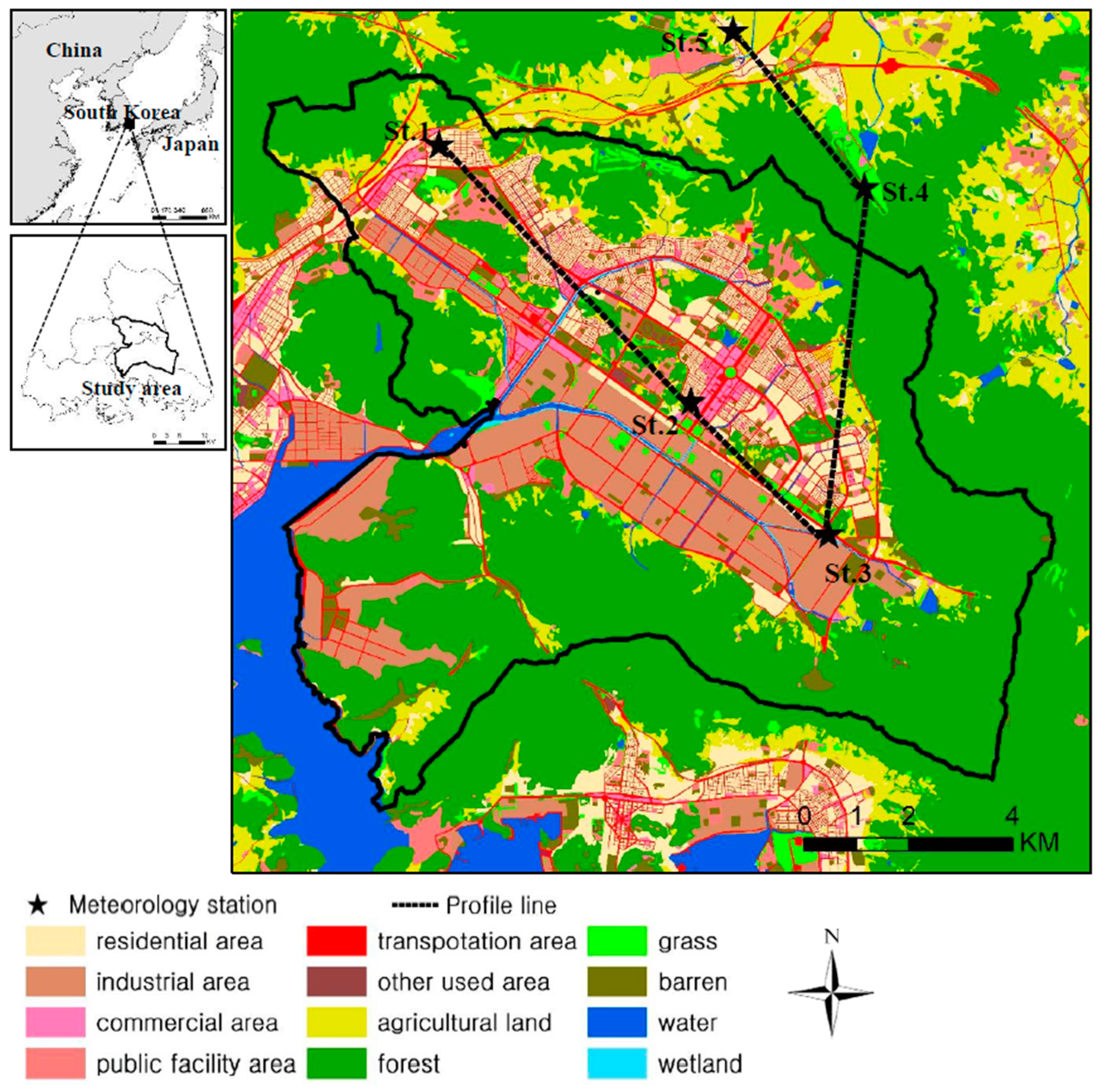
To determine whether the air temperature data should be simultaneously measured with the ASTER satellite, five stations (Sts. 1–5) from among the automatic meteorological measurement equipment installation stations managed by the Disaster and Safety Countermeasures Headquarters of Changwon City were selected at different locations in the study area (Figure 2). Air temperature at the meteorological station is collected in units of 1 min. Sts. 1–3 are inside urban areas, although the characteristics of the surrounding land use are different. Sts. 4 and 5, on the other hand, re outside the city. The automatic meteorological measurement equipment was installed >10 m above the ground on the roofs of regional community service centers. The data were obtained by connecting to the homepage of the Changwon City Disaster Safety Center (http://bangjae.changwon.go.kr) [44] and selecting the temperature data measured at the time of the ASTER satellite image acquisition.

2.2.3. Spatial Data

A land use status map, DSMs, and building data were collected for spatial data. The landcover classification map produced in 2010 by the Ministry of Environment of the Republic of Korea was used for the land use status map (Figure 2). This map was produced by first classifying the landcover using Landsat satellite imagery with a spatial resolution of 30 m, a digital topography map with a resolution of 1:25,000, and satellite imagery obtained from the Korea Multipurpose Satellite-2 (Kompsat-2) with a resolution of 4 m and then verifying the accuracy of the classification through field surveys (http://egis.me.go.kr). Landcover consists of 22 types such as residential areas, industrial areas, agricultural lands, and forests. The DSMs utilized the data collected by aerial light detection and ranging (LiDAR) in 2010 with a spatial resolution of 1 m × 1 m. The building data were obtained by extracting building layers from a 1:1000 digital topography map.

2.3. Analysis of Spatiotemporal Characteristics of Urban Temperature

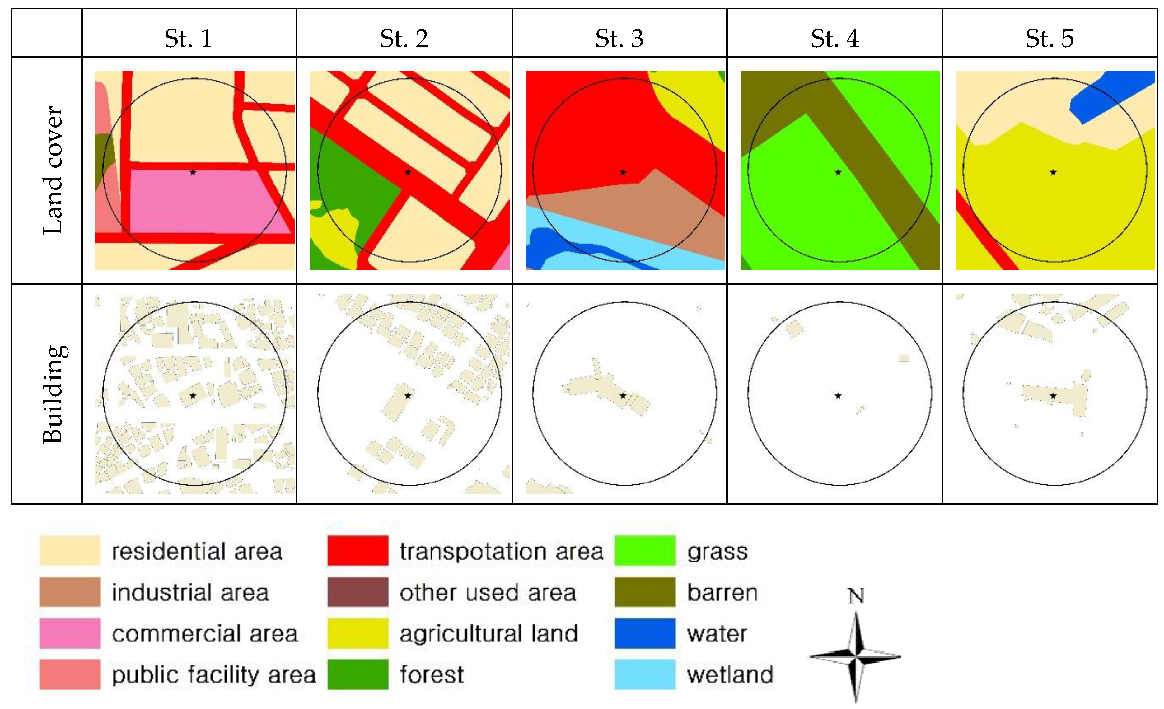
To identify the characteristics of spatiotemporal urban temperature, we performed three different analyses. First, we derived the spatiotemporal characteristics of urban temperature using the land-use types and building density in the area within a 90-m radius around the in situ observation point, DSM-based building heights, air temperature, and ASTER LST data. The radius of the in situ air temperature measurement point was set to 90 m to match the spatial resolution to that of the ASTER LST. Then, we derived the correlation between LST and air temperature during the daytime and nighttime by performing a linear regression analysis of LST and air temperature.
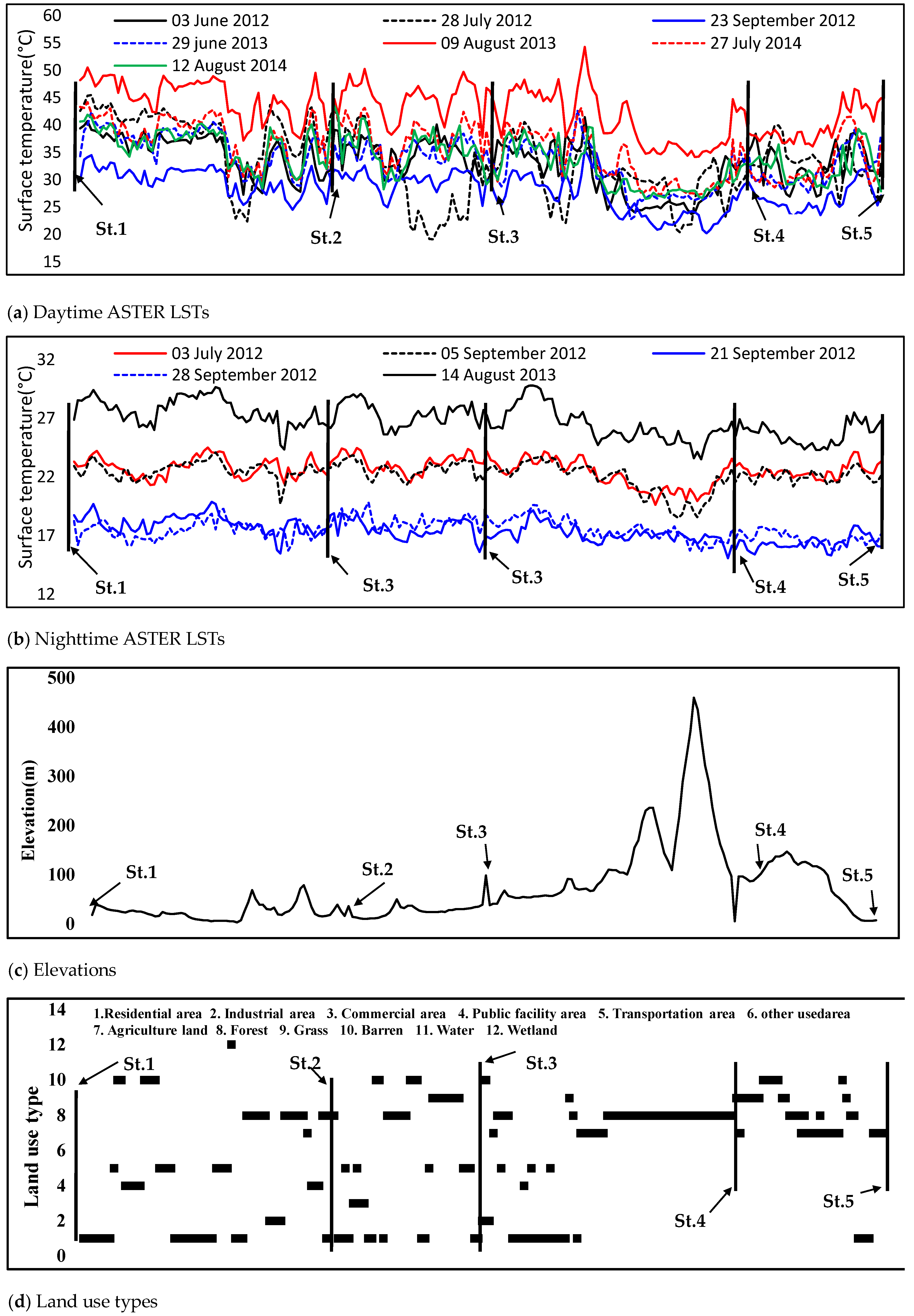
Second, we conducted a profile analysis to identify in more detail the LST characteristics according to land use type and altitude. Specifically, we plotted lines connecting the meteorological measurement points as shown in Figure 3, and segmented them at 90-m intervals to match the spatial resolution to that of the ASTER LST. Using the zonal statistic tool of ArcGIS 10.2 program, we constructed models for time-dependent mean ASTER LST, altitude, and typical land-use types.
Third, we analyzed the area ratio of each land use types and mean ASTER LSTs distributed within a Vector GRIDs (90 m × 90 m). For the analysis, we built a Vector GRID identical to the spatial resolution of ASTER LST data and put together information on the time-dependent ASTER LST and area ratio by land-use type in each grid. Drawing on previous research, we categorized land use into three types: urban land, cropland and barren land, and woodland. Based on the information contained in the Vector GRID, we analyzed the effect of land-use types depending on season and time of day and compared the analysis results with those of previous research in an attempt to derive a methodology for applying them to urban planning aimed to mitigate the UHI effect.

3. Results and Discussion

3.1. Spatial Characteristics Surrounding Meteorological Measurement Stations

Figure 3 shows the land use types and building distributions within 90 m around the meteorological measurement stations. The land use types were classified as built-up and natural areas. The built-up area consists of artificial covering materials such as residential, commercial, and industrial areas, while the natural area consists of natural covering materials such as agricultural, forest, and barren areas. The buildings were mainly investigated through the area ratio and average height.
The built-up area occupies the majority (i.e., 98.72%) of the area around St. 1. The building area was 36.71%, and the average building height was 8.54 m where low-rise buildings were concentrated. The area around St. 2 consists of 79.65% and 20.35% built-up and natural areas, respectively, and is adjacent to a forest area. The building area is 20.52%, and the average building height 7.53 m, which is similar to the building distribution characteristics around St. 1. The area around St. 3 consists of 87.09% and 12.91% built-up and natural areas, respectively, and is adjacent to a stream. Although the building area is small (i.e., 5.82%), the buildings are as high as 10.81 m. The area around St. 4 does not have any built-up area and only shows a small building area (i.e., 1.11%). The area around St. 5 consists of more natural areas (i.e., 75.95%) than urban ones (i.e., 24.05%) and shows a building area of 8.92%, consisting of low-density low-rise buildings (whose average height is 9.17 m) distributed throughout the area. Although most of the meteorological measurement stations were within an elevation of 40 m, St. 4 was installed at 96.57 m, the highest elevation (Table 2).

3.2. Characteristics of Urban Temperature

3.2.1. Air Temperature

Table 3 shows the temperatures measured at the various meteorological measurement stations. No temperatures were measured for some days at Sts. 4 and 5. The highest temperature (an average of 34.9 °C) was measured during the daytime on 28 August 2014 followed by 28 July 2012, 12 August 2014, and 27 July 2014 (averages of 34.7 °C, 30.6 °C, and 30.3 °C, respectively). The low temperature days were 3 June and 23 September 2012 (averages of 25.9 °C and 26.6 °C, respectively), and 29 June 2013 (an average of 29.4 °C). In Korea, June is the month when the daytime is the longest of the year owing to the highest altitude of the sun in the sky and to the rainfall that often occurs during the rainy season. The full-scale summer season begins in July, and the hot weather continues until August. The temperature gradually decreases from September and into autumn. The temperatures measured in July and August were the highest, which reflect the seasonal characteristics of Korea. The average nighttime temperature was the highest (i.e., 27.2 °C) on 14 August 2013, followed by 25.8 °C on 5 September 2012. During these months, the nights were tropical as the temperature remained around 25 °C or higher even late at night. The nighttime temperature was also high from July to early September, similar to the daytime temperature pattern, after which the temperature gradually decreased.
Comparing the temperatures by measurement station, the daytime temperature was the highest at St. 1. In particular, the temperatures on 9 August 2013 and 28 July 2012 were very high (i.e., above 35 °C) at 35.6 °C and 35.7 °C, respectively. To reiterate, St. 1 is located in a dense residential area. Sts. 2–4, on the other hand, showed lower daytime temperatures. Although Sts. 2 and 3 are located in residential areas, some commercial and industrial areas, urban parks, and streams are distributed in the adjacent areas. Furthermore, St. 4 is located in the mountains, thus the temperatures measured at Sts. 2–4 would be lower by about 1–2 °C than those measured at St. 1 because the natural land use type around Sts. 2–4 would reduce the surrounding temperatures. The temperature measured at St. 3 (i.e., 23.4 °C) was low in the daytime but high at nighttime, a difference of about 1–2 °C compared with those measured at the other stations. Sts. 2, 4, and 5 showed low nighttime temperatures. Sts. 4 and 5, which are located in the suburbs of the city, showed temperature differences of about 2–3 °C compared with the temperatures measured in the urban area. On 28 September 2012, the difference between the average temperature measured in the urban area and that measured in the suburban area was the largest (3.5 °C), while on 3 July and 5 September 2012, that difference was the smallest (i.e., 1.8 °C).
These results showed that urban areas comprised of artificial landcover materials showed higher temperatures than suburban areas, which showed the same tendency on all summer days. In addition, natural materials such as forests and streams reduced temperatures inside the urban areas.

3.2.2. Land Surface Temperature

Table 4 shows the results of the analysis of the LST measured within a 90-m radius around the meteorological measurement stations. The average daytime LST was the highest at 46.0 °C on 9 August 2013, followed by 39.7 °C on 27 July 2014, which showed the same LST characteristics. The lowest LST was 29.8 °C on 3 September 2012. Although the air temperature at St. 2 (29.7 °C) was lower than at the other stations, the LST there was the highest, probably because of the dense artificial landcover material there. On the contrary, the low air temperature at St. 2 was probably owing to the cooling effects of the adjacent forest area. The green areas distributed in the urban area helped decrease the air temperature. Sts. 3 and 4 showed low air temperature and LST. The difference between the highest LST and the lowest averaged 7.6 °C, which was greater than that of the air temperature (2.9 °C).
The average nighttime LST was 21.5 °C, which was 0.1 °C higher than the average nighttime air temperature (21.4 °C). The lowest daytime LST was 17.2 °C on both 21 and 28 September 2012. The air temperature was also the lowest at those times (i.e., 21 September 2012: 17.2 °C; and 28 September 2012: 17.3 °C). The air temperatures were higher than the LST ones on all days except 14 August 2013. However, during the daytime, the LST were higher than the air temperatures at all the stations because solar radiation was constantly shining down during the daytime, thereby heating the surfaces. The LST rapidly decreased during the nighttime, on the other hand, because solar radiation was absent and the artificial landcover material had a lower capacity for retaining the daytime heat [45]. Thus, the air temperature was higher than the LST during the nighttime, causing the surface temperature to decrease faster than the air temperature. Adjacent to a forest, St. 5 shows that the surface temperature was higher than the air temperature during the nighttime.

3.2.3. Correlation between Air Temperature and LST

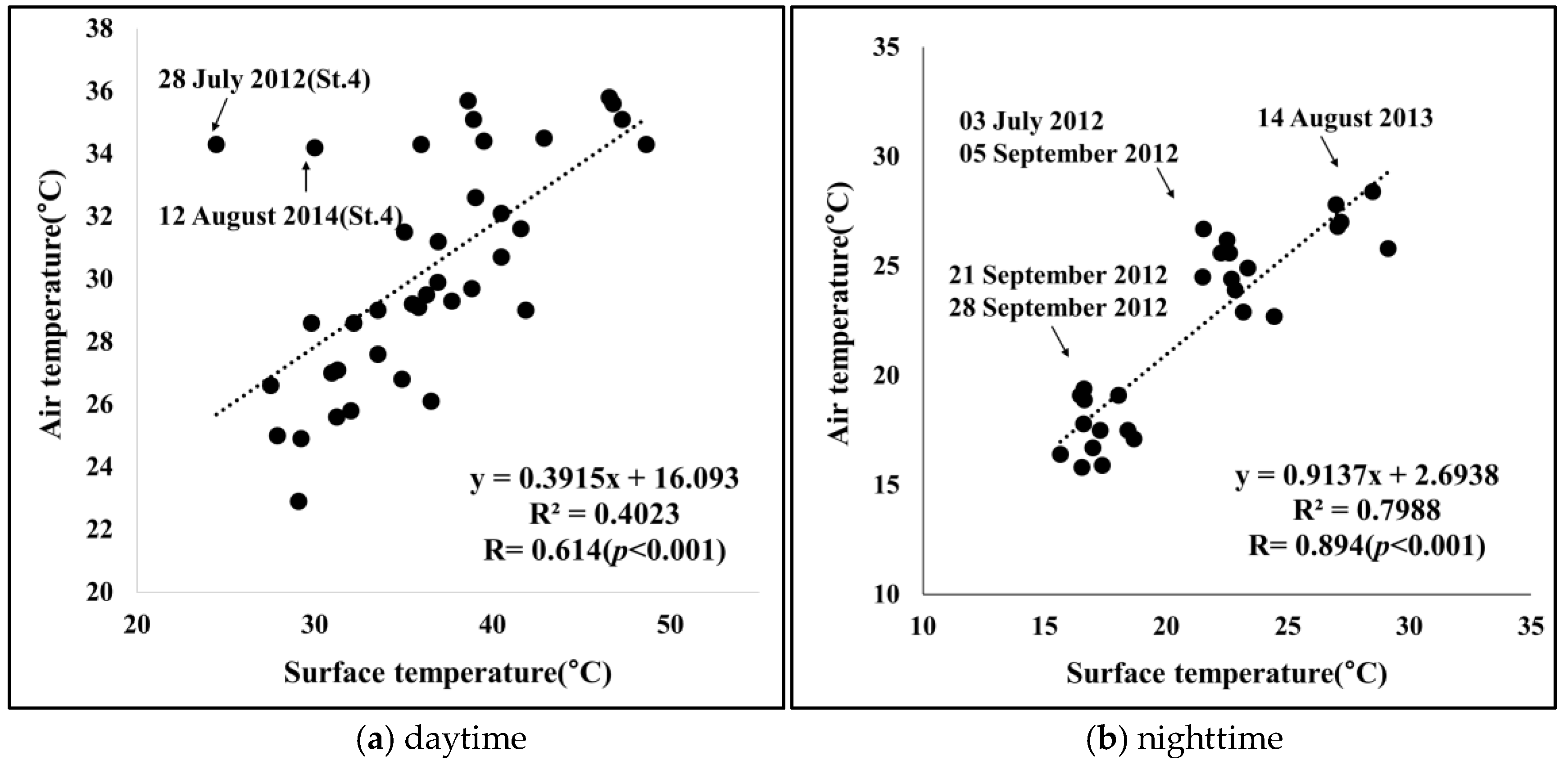
Figure 4 shows scatterplots for the air temperature and LST measured at the meteorological measurement stations on various days to analyze the relationship between the air temperature and LST. The Pearson Correlation Coefficient (R) of the daytime LST and air temperatures was 0.614 (p < 0.001), indicating that the air temperature increased with increasing LST. The slope of the linear regression equation was 0.3915. When the LST increased by 1 °C, the air temperature increased by 0.3915 °C, indicating that the air temperature increased less than the LST. The data mostly showed that the higher is the LST, the higher is the air temperature. However, on 28 July 2012 and 12 August 2014, the air temperature was high despite the low LST. The LST at St. 4 was low owing to the influence of cloud cover on the ASTER LST measurements.
During the nighttime, the correlation between the air temperature and LST was higher than that between them during the daytime (R = 0.894, p < 0.001). In addition, since the slope of the linear regression equation was near 1 (i.e., slope = 0.9137), the LST and air temperatures both increased similarly. The air temperature remained high during the daytime, resulting from the increase in the LST of the landcover material owing to solar radiation. However, the air temperature did not increase as rapidly as the LST owing to the influence of the atmospheric humidity and wind. Thus, the LST increased more than the air temperature. However, since solar radiation does not shine down during the nighttime, the surface heat radiated into the air, and thermal equilibrium was established and maintained after a certain amount of time, resulting in similar increases in LST and air temperatures. Meanwhile, the nighttime LST distribution was grouped according to specific days, resulting in a significant difference between the nighttime and daytime LST distributions.
The correlation between the LST and air temperatures is useful for analyzing the spatial patterns of UHI phenomena since it can predict the temperature distributions of urban areas from the LST data of satellite imagery. Many studies have analyzed correlations between LST and air temperatures from satellite imagery. Sun et al. [46] predicted air temperatures using MODIS LSTs and the crop water stress index (CWSI) for four meteorological stations on the North China Plain and showed that more than 80% of the data were accurate to within 3 °C. Fu et al. [47] estimated temperatures using MODIS LSTs for alpine meadows in the Northern Tibetan Plateau, and the mean daytime LST was forecast to be <10% of the linear regression coefficient during the growing season and more than 40% during the rest of the year. Klok et al. [23] used 11 NOAA-AVHRR images to analyze the relationship between LST and air temperatures in Rotterdam, the Netherlands and found that the linear regression model was 81% accurate. Cheng et al. [48] used NOAA-AVHRR data for North Taiwan to predict air temperature based on LST data from changes in landcover, and the linear regression model showed 91.49%, 77.08%, 53.6%, and 87.51% accuracy for data from the built-up area, paddy fields, water pond, and vegetation, respectively. Compared to the accuracy of the linear regression model derived in other studies, that of the one derived in this study was relatively high, although there are some differences according to the target area, utilized satellite imagery data, and research methods. Therefore, it is believed that the air temperature, except for that measured at the meteorological measurement stations, can be roughly estimated using the LST data of the satellite imagery.

3.3. Relationship between Spatial Pattern and Urban Temperature

3.3.1. Temperature Profiles

The temperature profiles are shown in Figure 5. Overall, the daytime surface temperature was the highest on 9 August 2013 (red line). However, it was low on 23 September 2012 (blue line). The differences in nighttime LST were clearly divided according to the day. The highest nighttime LST was measured on 14 August 2013 (black line) followed by 3 July 2012 (red line) and 5 September 2012 (black dots), while the lowest nighttime LST was measured on both 21 (blue line) and 28 (blue dots) September 2012.
The LST changed in each zone. In particular, the daytime LST changed more significantly than the nighttime ones, which are attributed to the influence of spatial characteristics such as land use type and elevation on the land surface. The daytime and nighttime LST were compared according to spatial characteristics. According to the land use type, the daytime LST was the highest (37.69 °C) in the residential area followed by 36.47 °C and 36.32 °C in the public facility and industrial areas, respectively. The profiles obtained for the public facility and industrial areas were unreliable since fewer measurements (9 and 7, respectively) were made in those areas than in the areas for other land use types. However, the profile obtained for the residential area was reliable since it was based on 50 measurements. Most residential homes in South Korea are single-family dwellings with fewer than three stories and are mostly comprised of artificial covering materials such as concrete and cement with small green areas. Owing to the characteristics of such residential areas, the LST tends to be high resulting from the excessive accumulation of radiant heat from solar radiation during the daytime. The commercial, forest, and barren areas (whose LSTs were 30.89 °C, 31.85 °C, and 31.85 °C, respectively) were identified as low LST types. The profile obtained for the commercial area, which consists of three sample areas, must become more reliable by analyzing more commercial area types. The highest LST (36.34 °C) was measured in the flat areas between 0 and 50 m since most of the flat areas such as residential and industrial areas have built-up areas showing high LSTs. The LSTs at elevations above 100 m, on the other hand, were lower than 30 °C, suggesting that higher elevation areas are located outside the city, where forests showing lower LSTs are located (Table 5).
The difference in the nighttime LSTs among the various land use types was about 1 °C, which was less than the difference in the daytime LSTs among the same (~6 °C). The land use types associated with high LSTs were the transportation areas (including roads) (21.97 °C) and residential areas (21.86 °C), while the farming areas (which showed a high daytime LST) also showed a relatively high nighttime LST (21.68 °C). The industrial (20.84 °C), grass (20.59 °C), and barren (20.67 °C) areas all showed lower nighttime LSTs (Table 6). In particular, the industrial area showed a high daytime LST because the covering material was mostly metal, while the nighttime LST of the industrial area was low because the metal had rapidly cooled. The difference among the daytime and nighttime LSTs with respect to elevation was insignificant, only about 1 °C.
Since profile analyses only compare the LST characteristics according to the space for a given day for some regions through which the line passes, it has limitations when used to characterize an entire area. Residential, commercial, and industrial areas, where artificial covering materials are concentrated, showed high LSTs, while natural areas such as forest, agricultural, and grassland areas showed low ones. These results were consistent with previous research that analyzed the relationship between the spatial characteristics and the LST [10,48,49,50,51]. The results suggested that the higher is the elevation, the lower is the LST owing to the landcover types rather than to the elevation.

3.3.2. Relationship between Landcover Area Ratio and Urban Temperature

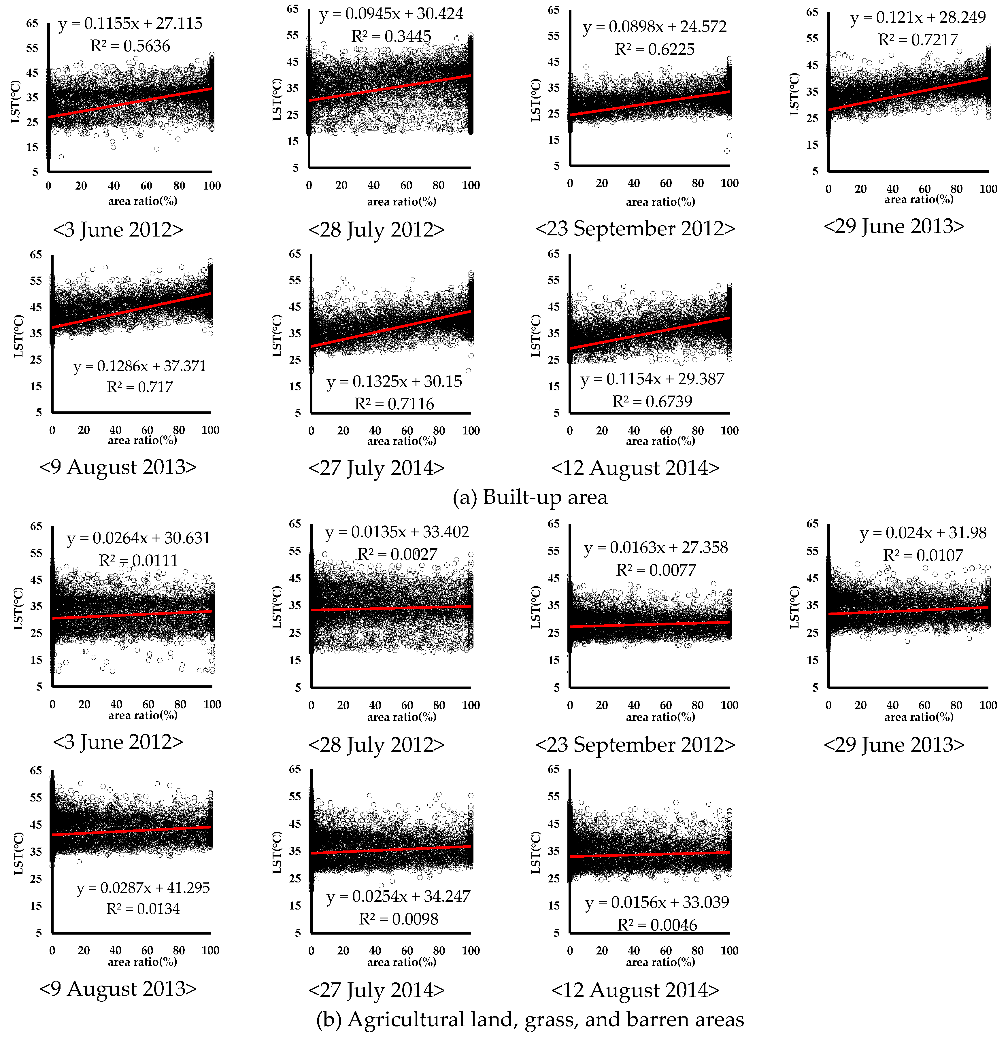
A scatterplot analysis was conducted to compare the LST characteristics by day according to the area ratio of land types categorized into urban, agricultural, barren, and forest areas. First, the results for the daytime LSTs are shown in Figure 6. Although the LST of the built-up area increased with increasing area ratio, it increased by varying degrees each day. The greatest increase was shown on 27 July 2014, when the slope of the linear regression model was 0.1325, suggesting that the LST increased by about 1.3 °C as the area ratio of the built-up area increased by 10%. This was followed by 9 August 2013 (slope = 0.1286) and 29 June 2013 (slope = 0.1210). On the other hand, 23 September 2012 showed a very low increase in daytime LST with increasing area ratio of the built-up area. The slope that day was only 0.0898, suggesting that the built-up area made the LST rise between June and August, during the peak of summer in Korea (Figure 6a).
For the agricultural and barren areas, the explanatory power (R2) of the linear regression model was <0.1. Therefore, the results of those analyses were unreliable, probably because of the surrounding LST since the urban area of Changwon City is not adjacent to any large-scale farmland—which is only present on a small scale near the built-up and forest areas (Figure 6b).
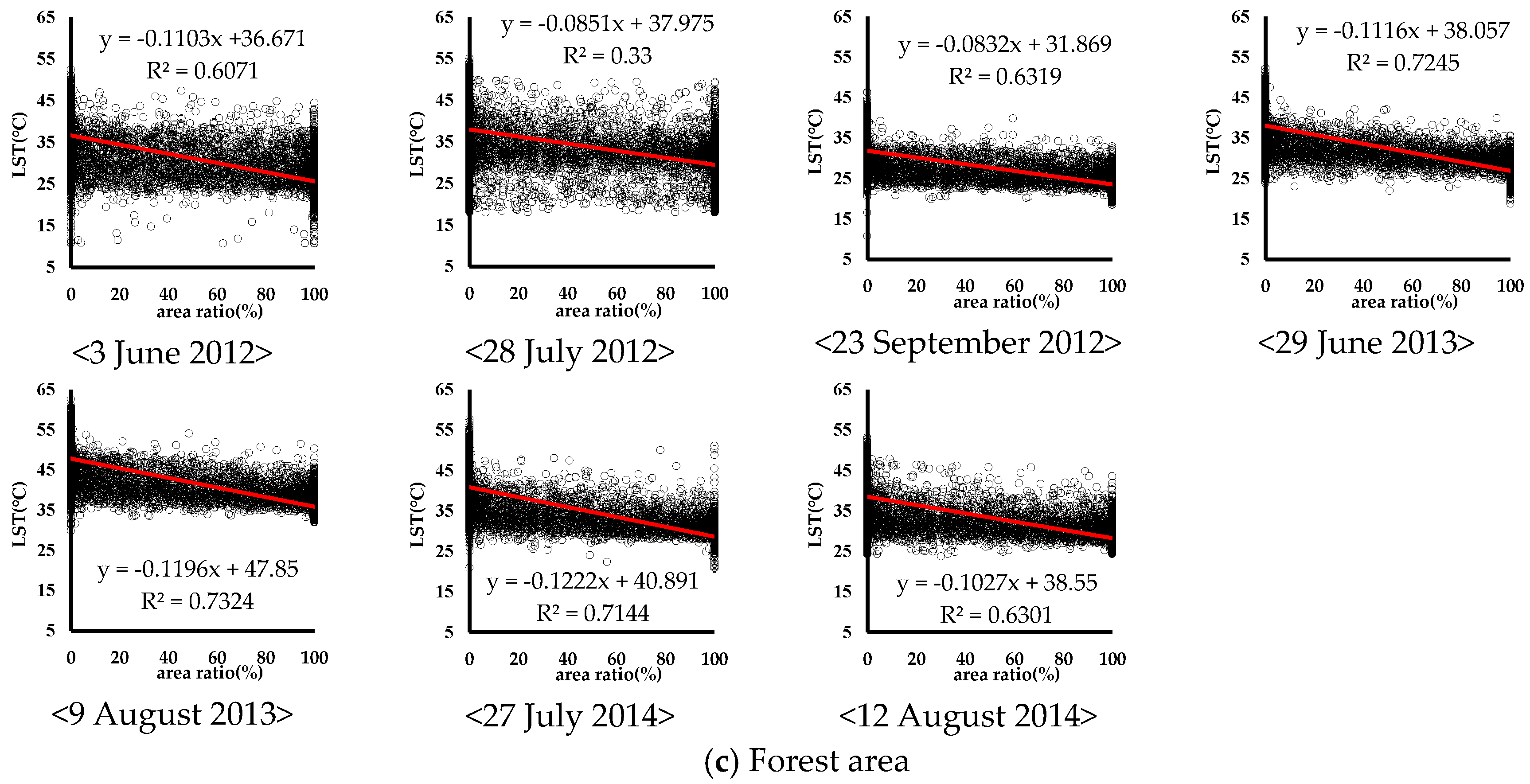
The LST of the forest area decreased with increasing area ratio. The greatest decrease in slope was observed on 27 July 2014 (slope = −0.1222), and the LST decreased by about 1.2 °C when the forest area increased by 10%, while 23 September 2013 showed a decrease (−0.0832), and the average decrease for the remaining time period was about −0.11 (3 June 2012: −0.1103; 29 June 2013: −0.1116; 9 August 2013: −0.1196; and 12 August 2014: −0.1027) (Figure 6c).
Meanwhile, 28 July 2012 showed low explanatory power in the linear regression model, resulting from the effect of cloud cover on the ASTER LST data measured that day.
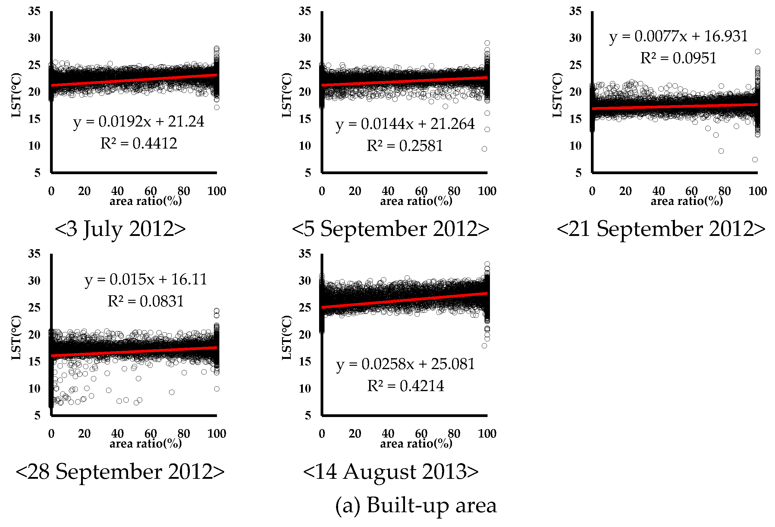
The corresponding results for the nighttime LSTs are shown in Figure 7. The explanatory power of the linear regression model for the nighttime LSTs was lower than that of the model for the daytime ones on all days. The slopes were also gentle because the changes in the LST with the area ratio were insignificant. Although the nighttime LST in the built-up area increased with increasing area ratio as did the daytime LST, the slope of the regression line for the nighttime LSTs was much gentler than that for the daytime ones. The steepest slope (0.0258) was recorded on 14 August 2012, when the LST increased by about 0.25 °C when the built-up area ratio increased by 10%. On the other hand, 21 September 2012 showed the gentlest slope (0.0077). The increase in LST in the built-up area was the most significant in August when the weather was the hottest and the nights were tropical (Figure 7a).
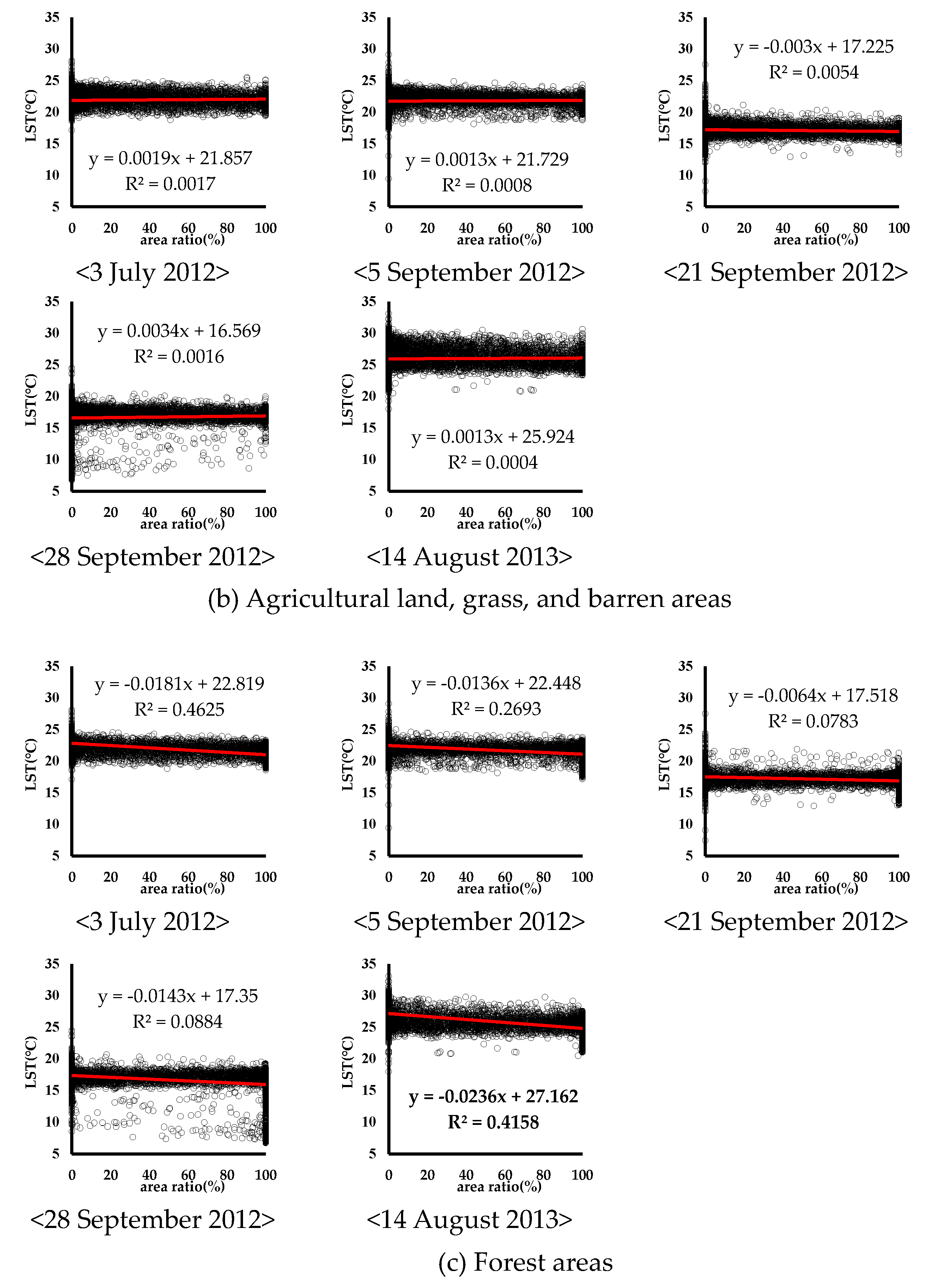
There were few changes in the LST owing to changes in the area ratio of the agricultural and barren areas. On 21 September 2012 (−0.0030), although the LST decreased with increasing area ratio, the LST increased on all other days (3 July 2012: 0.0019; 5 September 2012: 0.0013; 28 September 2012: 0.0034; and 14 August 2012: 0.0013). There were no distinct changes in the nighttime LSTs of the agricultural and barren areas (Figure 7b).
Although the nighttime LST of the forest area decreased with increasing area ratio, as did the daytime LST, the slope of the nighttime LST regression line was gentle, similar to that for the built-up area. The slope was the steepest (−0.0236) on 14 August 2012 and the gentlest (−0.0064) on 21 September 2012, and it showed the identical characteristics of the slope for the daytime LST (Figure 7c).

3.4. Discussion

The analysis results reveal that LST showed different characteristics in different spatial patterns depending on season and time of day. In particular, built-up areas showed the greatest increase in LST during the daytime in July and August, the two hottest months in South Korea. The tendency of LST decrease in forest areas was lower than the tendency of LST increase in built-up areas, which allows the assumption that the overall LST would increase provided that forest areas and built-up areas have the same area ratio. On 27 July 2014, for example, in an area composed of 10% forest area and 10% built-up area, if the area increase at the same ratio of 20% each, the forest area LST decreases by 2.44 °C, whereas the LST increases by 2.65 °C, resulting in an overall LST increase of 0.21 °C. Rise in LST leads to rise in air temperature, and the application of 0.21 °C increase in LST to the linear regression model for daytime LST and air temperature in Figure 4a yields 0.08 °C rise in air temperature. These results are meaningful because it can estimate the variation of LST and air temperature according to spatial pattern although uncertainty in not considered due to accuracy of satellite imagery and LST retrieval algorithm.
In previous research, there have been many studies on the relationship between land cover land use and LST. Pal and Ziaul [30] analyzed the relationship between land cover change and LST using Landsat TM for various periods in English Bazar Municipality. R2 between land cover change and LST was 0.4–0.6. The characteristics of land cover change and LST were different according to the periods. Zhao et al. [52] analyzed the relationship LST and land cover using Landsat 8 in Shenyang, China. The agricultural area showed a decrease of about 0.2037 °C according to the area ratio and R2 was 0.3533, which was similar to that of this study. The forest area was similar to the agricultural area at 0.2250 °C, but R2 was 0.5476 and the correlation was high. Tran et al. [37] analyzed the characteristics of urban area and LST by linear regression for various periods. R2 between of urban cover ratio and LST was 0.97–0.99. Klok et al. [23] conducted the relationship green space and LST in July, the mean LST decreased by 1.3 °C when green space increased by 10%. In the present study, the mean LST decreased by 2.3 °C under the same conditions, demonstrating a 1% higher LST reduction effect. As a result of comparing with the previous studies, the relationship of the LST and the land cover change was different according to the analyzed time and target area. This may be because the satellite images and spatial data used for analysis are different. However, another reason is that the effect of spatial patterns on urban temperature is different due to the geographical location and urban environment. When the geographical location and the urban environment are different, the amount of radiant energy from the sun and the thermal properties (emissivity, albedo, and heat capacity) are different. Therefore, to mitigate the UHI effect from the perspective of urban planning, it is essential to understand the impact of spatial pattern on the LST taking into account the urban environment and climatic characteristics.
As examined above, the correlation between surface temperature and spatial pattern is unclear during the nighttime, presumably because of the indistinct differences in the LST by land-use type due to the absence of solar radiation energy input. However, the heat of the surface accumulated during the daytime continues to affect the nighttime temperature, causing a phenomenon similar to tropical night. Accordingly, lowering the LST during the daytime is assumed to be effective during the nighttime. Zhou et al. [31] reported that 63% of the studies investigating the UHI phenomenon using satellite imagery involved daytime, 6% nighttime, and 30% both, demonstrating that much fewer studies have been dedicated to the nighttime UHI phenomenon. This is because the Landsat TM LST imagery, which is most widely used for LST analysis, is available only during the daytime. On this note, the results of the present study are significant in that they were obtained by analyzing the effects during both daytime and nighttime and comparing the characteristics of period-dependent urban temperature.

4. Conclusions

This study analyzed the characteristics of urban temperature depending on spatial patterns using ASTER LST data and spatial data from various time periods to highlight the need to set up an UHI effect mitigation plan taking into account urban environment and meteorological characteristics from the perspective of urban planning. To achieve this end, we analyzed the spatial characteristics of the in situ measurement point in different time periods and times of day and the relationship between LST and air temperature, and derived the characteristics of LST according to the area ratio by land-use type. Then, we compared the analysis results with those of previous research and established a methodology for applying those researches finding to setting up UHI effect mitigation plans.
As a result, the correlation between LST and air temperature during the daytime was found to have an accuracy rate of 60% when checked against the in situ measurements, similar to that of previous research, and 89.4% during the nighttime, which could not be compared with previous research for lack of studies involving nighttime LST. The daytime LST was found to rise in urban land to different extents depending on time of day, which was slightly different from the result of a comparable previous study. The nighttime LST did not show any distinct trend depending on spatial patterns. In addition, because of the lack of previous research data at nighttime because of the collection of satellite image data, we could not directly compare with the results of this study.
This study analyzed urban temperature characteristics for various time and period according to spatial pattern. Its main achievements are twofold: identification of urban temperature characteristics that vary depending on spatial patterns (land-use types) and time of day (daytime vs. nighttime) and determination of the impact of spatial patterns on urban temperature depending on urban environment and meteorological characteristics, differentiating itself from previous research. These results can be used as important source data for decision-making regarding UHI effect reduction from the perspective of urban planning. In particular, to mitigate the current UHI effect, indiscriminately creating green space or imposing restrictions on urban development activities can hamper a sustainable development of cities. The results of this study provide quantitative data on the impact of spatial patterns (land-use types) on the urban temperature in summer, i.e., at the peak of the UHI effect. They are expected to serve as important data that can help decision-making regarding urban planning and policy decision for mitigating the UHI effect at the stages of urban redevelopment and reconstruction.

Author Contributions

B.S. and K.P. conceived and designed the research; B.S. analyzed the spatial data and wrote the paper.

Funding

This work was supported by the National Research Foundation (NRF) of Korea grant funded by the Korea government (Ministry of Science and ICT) (No. NRF-2016R1A2B4015460).

Conflicts of Interest

The authors declare no conflicts of interest.

References

  1. Rizwan, A.M.; Dennis, L.Y.C.; Liu, C. A review on the generation, determination and mitigation of the Urban Heat Island. J. Environ. Sci. 2008, 20, 120–128. [Google Scholar] [CrossRef]
  2. Adams, M.P.; Smith, P.L. A systematic approach to model the influence of the type and density of vegetation cover on urban heat using remote sensing. Landsc. Urban Plan 2014, 132, 47–54. [Google Scholar] [CrossRef]
  3. Phelan, P.E.; Kaloush, K.; Miner, M.; Golden, J.; Phelan, B.; Silva, I.I.I.H.; Taylor, R.A. Urban heat island: Mechanisms, implications, and possible remedies. Annu. Rev. Environ. Resour. 2015, 40, 285–307. [Google Scholar] [CrossRef]
  4. Levermore, G.; Parkinson, J.; Lee, K.; Laycock, P.; Lindley, S. The increasing trend of the urban heat island intensity. Urban Clim. 2018, 24, 360–368. [Google Scholar] [CrossRef]
  5. Santamouris, M. Using cool pavements as a mitigation strategy to fight urban heat island-a review of the actual development. Renew. Sustain. Energy Rev. 2013, 26, 224–240. [Google Scholar] [CrossRef]
  6. Jamei, E.; Rajagopalan, P.; Seyedmahmoudian, M.; Jamei, Y. Review on the impact of urban geometry and pedestrian level greening on outdoor thermal comfort. Renew. Sustain. Energy Rev. 2016, 54, 1002–1017. [Google Scholar] [CrossRef]
  7. Tan, J.; Zheng, Y.; Tang, X.; Guo, C.; Li, L.; Song, G.; Zhen, X.; Yuan, D.; Kalkstein, A.J.; Li, F.; et al. The urban heat island and its impact on heat waves and human health in Shanghai. Int. J. Biometeorol. 2010, 54, 75–84. [Google Scholar] [CrossRef] [PubMed]
  8. Coseo, P.; Larsen, L. How factors of land use/land cover, building configuration, and adjacent heat sources and sinks explain Urban Heat Islands in Chicago. Landsc. Urban. Plan. 2014, 125, 117–129. [Google Scholar] [CrossRef]
  9. Wang, W.; Liu, K.; Tang, R.; Wang, S. Remote sensing image-based analysis of the urban heat island effect in Shenzhen, China. Phys. Chem. Earth 2019. [Google Scholar] [CrossRef]
  10. Schwarz, N.; Schlink, U.; Franck, U.; Großmann, K. Relationship of land surface and air temperatures and its implications for quantifying urban heat island indicators-An application for the City of Leipzig (Germany). Ecol. Indic. 2012, 18, 693–704. [Google Scholar] [CrossRef]
  11. Pongracz, R.; Bartholy, J.; Dezso, Z. Application of remotely sensed thermal information to urban climatology of Central European cities. Phys. Chem. Earth 2010, 35, 95–99. [Google Scholar] [CrossRef]
  12. Weng, Q. Thermal infrared remote sensing for urban climate and environmental studies: Methods, applications, and trends. ISPRS J. Photogramm. Remote Sens. 2009, 64, 335–344. [Google Scholar] [CrossRef]
  13. Yang, Q.; Huang, X.; Tang, Q. The footprint of urban heat island effect in 302 Chinese cities: Temporal trends and associated factors. Sci. Total Environ. 2019, 655, 652–662. [Google Scholar] [CrossRef] [PubMed]
  14. Voogt, J.A.; Oke, T.R. Thermal remote sensing of urban climates. Remote Sens. Environ. 2003, 86, 370–384. [Google Scholar] [CrossRef]
  15. Grimmond, S. Urbanization and global environmental change: Local effects of urban warming. Geogr. J. 2007, 173, 83–88. [Google Scholar] [CrossRef]
  16. Martin, P.; Baudouin, Y.; Gachon, P. An alternative method to characterize the surface urban heat island. Int. J. Biometeorol. 2015, 59, 849–861. [Google Scholar] [CrossRef]
  17. Jamei, Y.; Rajagopalan, P.; Sun, Q. Spatial structure of surface urban heat island and its relationship with vegetation and built-up areas in Melbourne, Australia. Sci. Total Environ. 2019, 659, 1335–1351. [Google Scholar] [CrossRef]
  18. Li, J.; Song, C.; Cao, L.; Zhu, F.; Meng, X.; Wu, J. Impacts of landscape structure on surface urban heat islands: A case study of Shanghai, China. Remote Sens. Environ. 2011, 115, 3249–3263. [Google Scholar] [CrossRef]
  19. Weng, Q.; Lu, D.; Schubring, J. Estimation of land surface temperature–vegetation abundance relationship for urban heat island studies. Remote Sens. Environ. 2004, 89, 467–483. [Google Scholar] [CrossRef]
  20. Yuan, F.; Bauer, M.E. Comparison of impervious surface area and normalized difference vegetation index as indicators of surface urban heat island effects in Landsat imagery. Remote Sens. Environ. 2007, 106, 375–386. [Google Scholar] [CrossRef]
  21. Duncan, J.M.A.; Boruff, B.; Saunders, A.; Sun, Q.; Hurley, J.; Amati, M. Turning down the heat: An enhanced understanding of the relationship between urban vegetation and surface temperature at the city scale. Sci. Total Environ. 2019, 656, 118–128. [Google Scholar] [CrossRef] [PubMed]
  22. Chen, X.-L.; Zhao, H.-M.; Li, P.-X.; Yin, Z.-Y. Remote sensing image-based analysis of the relationship between urban heat island and land use/cover changes. Remote Sens. Environ. 2006, 104, 133–146. [Google Scholar] [CrossRef]
  23. Klok, L.; Zwart, S.; Verhagen, H.; Mauri, E. The surface heat island of Rotterdam and its relationship with urban surface characteristics. Resour. Conserv. Recycl. 2012, 64, 23–29. [Google Scholar] [CrossRef]
  24. Benali, A.; Carvalho, A.C.; Nunes, J.P.; Carvalhais, N.; Santos, A. Estimating air temperature in Portugal using MODIS LSAT data. Remote Sens. Environ. 2012, 124, 108–121. [Google Scholar] [CrossRef]
  25. Kloog, I.; Chudnovsky, A.; Koutrakis, P.; Schwartz, J. Temporal and spatial assessments of minimum air temperature using satellite surface temperature measurements in Massachusetts, USA. Sci. Total Environ. 2012, 432, 85–92. [Google Scholar] [CrossRef] [Green Version]
  26. Coutts, A.M.; Harris, R.J.; Phan, T.; Livesley, S.J.; Williams, N.S.G.; Tapper, N. Thermal infrared remote sensing of urban heat: Hotspots, vegetation, and an assessment of techniques for use in urban planning. Remote Sens. Environ. 2016, 186, 637–651. [Google Scholar] [CrossRef]
  27. Wang, Y.C.; Hu, B.K.H.; Myint, S.W.; Feng, C.C.; Chow, W.T.L.; Passy, P.F. Patterns of land change and their potential impacts on land surface temperature change in Yangon, Myanmar. Sci Total Environ. 2018, 643, 738–750. [Google Scholar] [CrossRef]
  28. Ferreira, L.S.; Duarte, D.H.S. Exploring the relationship between urban form, land surface temperature and vegetation indices in a subtropical megacity. Urban. Clim. 2019, 27, 105–123. [Google Scholar] [CrossRef]
  29. Hereher, M.E. Effect of land use/cover change on land surface temperatures—The Nile Delta, Egypt. J. Afr. Earth Sci. 2017, 126, 75–83. [Google Scholar] [CrossRef]
  30. Pal, S.; Ziaul, S. Dection of land use and land cover change and land surface temperature in English Bazar urban centre. Egypt. J. Remote Sens. 2017, 20, 125–145. [Google Scholar] [CrossRef]
  31. Zhou, D.; Xiao, J.; Bonafoni, S.; Berger, C.; Deilami, K.; Zhou, Y.; Frolking, S.; Yao, R.; Qiao, Z.; Sobrino, J.A. Satellite Remote Sensing of Surface Urban Heat Islands: Progress, Challenges, and Perspectives. Remote Sens. 2019, 11, 48. [Google Scholar] [CrossRef]
  32. Zhang, P.; Bounoua, L.; Imhoff, M.L.; Wolfe, R.E.; Thome, K. Comparison of MODIS land surface temperature and air temperature over the continental USA meteorological stations. Can. J. Remote Sens. 2014, 40, 110–122. [Google Scholar] [CrossRef]
  33. Sun, H.; Chen, Y.; Zhan, W. Comparing surface-and canopy-layer urban heat islands over Beijing using MODIS data. Int. J. Remote Sens. 2015, 36, 5448–5465. [Google Scholar] [CrossRef]
  34. Azevedo, J.A.; Chapman, L.; Muller, C.L. Quantifying the daytime and night-time urban heat island in Birmingham, UK: A comparison of satellite derived land surface temperature and high resolution air temperature observations. Remote Sens. 2016, 8, 153. [Google Scholar] [CrossRef]
  35. Li, L.; Huang, X.; Li, J.; Wen, D. Quantifying the spatiotemporal trends of canopy layer heat island (CLHI) and its driving factors over Wuhan, China with satellite remote sensing. Remote Sens. 2017, 9, 536. [Google Scholar] [CrossRef]
  36. Sheng, L.; Tang, X.; You, H.; Gu, Q.; Hu, H. Comparison of the urban heat island intensity quantified by using air temperature and Landsat land surface temperature in Hangzhou, China. Ecol. Indic. 2017, 72, 738–746. [Google Scholar] [CrossRef]
  37. Tran, D.X.; Pla, F.; Latorre-Carmona, P.; Myint, S.W.; Caetano, M.; Kieu, H.V. Characterizing the relationship between land use land cover change and land surface temperature. ISPRS J. Photogramm. Remote Sens. 2017, 124, 119–132. [Google Scholar] [CrossRef] [Green Version]
  38. Song, B.G.; Park, K.H. Contribution of greening and high-albedo coatings to improvements in the thermal environment in complex urban areas. Adv. Meteorol. 2015, 14, 792172. [Google Scholar] [CrossRef]
  39. Song, B.G.; Kim, G.A.; Seo, K.H.; Lee, S.W.; Park, K.H. Analysis of Surface Temperature Characteristics by Land Surface Fabrics Using TIR Images. J. Korean Assoc. Geogr. Inf. Stud. 2018, 21, 162–175. [Google Scholar]
  40. Song, B.G.; Park, K.H. Air Ventilation Evaluation at Nighttime for the Construction of Wind Corridor in Urban Area. J. Korean Assoc. Geogr. Inf. Stud. 2013, 16, 16–29. [Google Scholar] [CrossRef]
  41. Song, B.G.; Park, K.H. Validation of ASTER Surface Temperature Data with In Situ Measurements to Evaluate Heat Islands in Complex Urban Areas. Adv. Meteorol. 2014, 620410. [Google Scholar] [CrossRef]
  42. Hartz, D.A.; Prashad, L.; Hedquist, B.C.; Golden, J.; Brazel, A.J. Linking satellite images and hand-held infrared thermography to observed neighborhood climate conditions. Remote Sens. Environ. 2006, 104, 190–200. [Google Scholar] [CrossRef]
  43. Gillespie, A.; Rokugawa, S.; Matsunaga, T.; Cothern, J.S.; Hook, S.; Kahle, A.B. A Temperature and Emissivity Separation Algorithm for Advanced Spaceborne Thermal Emission and Reflection Radiometer (ASTER) Images. IEEE Trans. Geosci. Remote Sens. 1998, 36, 1113–1126. [Google Scholar] [CrossRef]
  44. Homepage of Disaster and Safety Countermeasures Headquarters of Changwon City. Available online: http://bangjae.changwon.go.kr (accessed on 15 February 2019).
  45. Weber, S. Comparison of in-situ measured ground heat fluxes within a heterogeneous urban ballast layer. Theor. Appl. Climatol. 2006, 83, 169–179. [Google Scholar] [CrossRef]
  46. Sun, Y.J.; Wang, J.F.; Zhang, R.H.; Gillies, R.R.; Xue, Y.; Bo, Y.C. Air temperature retrieval from remote sensing data based on thermodynamics. Theor. Appl. Climatol. 2005, 80, 37–48. [Google Scholar] [CrossRef]
  47. Fu, G.; Shen, Z.; Zhang, X.; Shi, P.; Zhang, Y.; Wu, J. Estimating air temperature of an alpine meadow on the Northern Tibetan Plateau using MODIS land surface temperature. Acta Ecol. Sin. 2011, 31, 8–13. [Google Scholar] [CrossRef]
  48. Cheng, K.S.; Su, Y.F.; Kuo, F.T.; Hung, W.C.; Chiang, J.L. Assessing the effect of landcover changes on air temperature using remote sensing images—A pilot study in northern Taiwan. Landsc. Urban. Plan 2008, 85, 85–96. [Google Scholar] [CrossRef]
  49. Takebayashi, H.; Moriyama, M. Study on the urban heat island mitigation effect achieved by converting to grass-covered parking. Sol. Energy 2009, 83, 1211–1223. [Google Scholar] [CrossRef] [Green Version]
  50. Nichol, J.E.; Fung, W.Y.; Lam, K.; Wong, M.S. Urban heat island diagnosis using ASTER satellite images and ‘in situ’ air temperature. Atmos. Res. 2009, 94, 276–284. [Google Scholar] [CrossRef]
  51. Ng, E.; Chen, L.; Wang, Y.; Yuan, C. A study on the cooling effects of greening in a high-density city: An experience from Hong Kong. Build. Environ. 2012, 47, 256–271. [Google Scholar] [CrossRef]
  52. Zhao, Z.Q.; He, B.J.; Li, L.G.; Wang, H.B.; Darko, A. Profile and concentric zonal analysis of relationship between land use/land cover and land surface temperature: Case study of Shenyang, China. Energ. Build. 2017, 155, 282–295. [Google Scholar] [CrossRef]
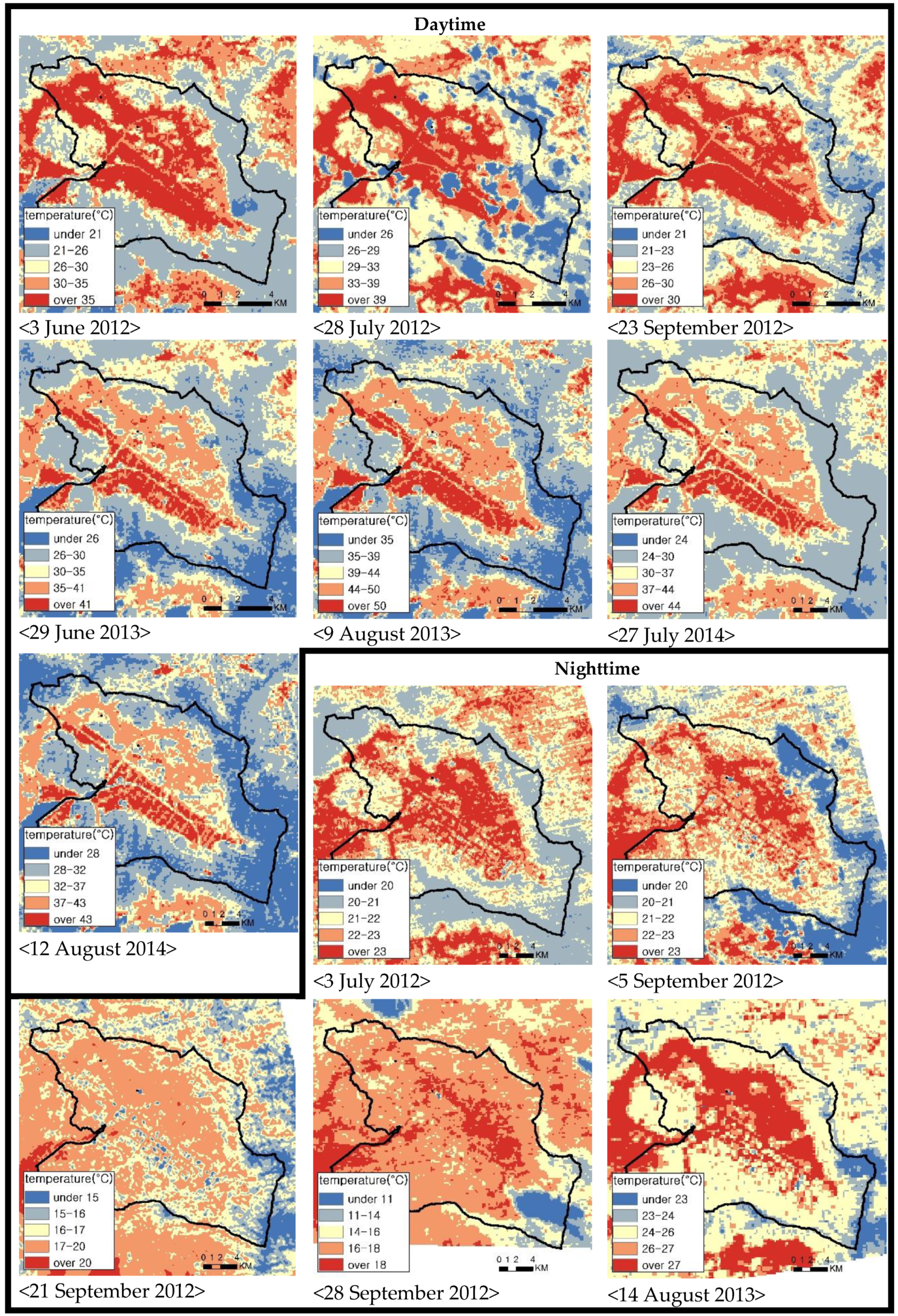
Figure 1. Daytime and nighttime ASTER LST images.
Sustainability 11 03777 g001
Figure 2. Land use types, meteorological measurement stations, and profile line status of research area.
Sustainability 11 03777 g002
Figure 3. Land use types and building distributions surrounding meteorological measurement stations.
Sustainability 11 03777 g003
Figure 4. Pearson Correlation Coefficients (R) and scatterplots of LST and air temperatures measured during: (a) daytime; and (b) nighttime.
Sustainability 11 03777 g004
Figure 5. Profiles obtained for: (a) daytime ASTER LSTs; (b) nighttime ASTER LSTs; (c) elevations; and (d) land use types.
Sustainability 11 03777 g005
Figure 6. Scatterplot analyses of daytime ASTER LSTs for various days for: (a) built-up; (b) agricultural land, grass, and barren; and (c) forest areas.
Sustainability 11 03777 g006aSustainability 11 03777 g006b
Figure 7. Scatterplot analyses of corresponding nighttime ASTER LSTs for various days for: (a) built-up; (b) agricultural land, grass, and barren; and (c) forest areas.
Sustainability 11 03777 g007aSustainability 11 03777 g007b
Table 1. List of ASTER LST data collected.
TimeDateLocal Time (UTC + 9)
Daytime3 June 201214:19
28 July 201214:10
23 September 201214:16
29 June 201314:21
9 August 201314:20
27 July 201414:18
12 August 201414:22
Nighttime3 July 201201:35
5 September 201201:34
21 September 201201:31
28 September 201201:37
14 August 201301:33
Table 2. Characteristics of Land use, building, and elevation within 90 m around the meteorological measurement point.
StationArea Ratio of Land Use (%)BuildingElevation (m)
UrbanNaturalArea Ratio (%)Mean Height
St. 198.721.2836.718.5423.66
St. 279.6520.3520.527.5314.26
St. 387.0912.915.8210.8139.16
St. 40.00100.001.116.7596.57
St. 524.0575.958.929.1711.60
Table 3. Air temperatures (°C) measured at meteorological measurement stations.
StationDaytimeNighttime
201220132014Mean20122013Mean
3 June28 July23 September29 June9 August27 July12 August3 July5 September21 September28 September14 August
St. 126.835.727.129.535.632.130.731.123.925.617.517.827.022.4
St. 226.134.425.629.134.329.029.329.722.724.917.117.525.821.6
St. 325.034.328.629.034.529.734.230.824.426.719.119.127.823.4
St. 425.8-24.9--29.228.627.122.9-15.815.9-18.2
St. 5-34.326.629.935.131.630.431.3-25.616.716.426.821.4
Mean25.934.726.629.434.930.330.630.023.525.717.217.326.921.4
Max.–Min.2.61.43.72.21.53.65.62.91.81.83.33.52.62.6
Table 4. LST (°C) measured at various meteorological measurement stations.
StationDaytimeNighttime
201220132014Mean20122013Mean
3 June28 July3 September29 June9 August27 July12 August3 July5 September21 September28 September14 August
St. 134.938.631.336.346.840.540.538.422.822.617.316.627.221.3
St. 236.639.531.235.848.741.937.738.824.423.418.718.429.122.8
St. 327.924.529.833.642.938.830.032.522.721.516.518.027.021.1
St. 432.029.129.235.044.235.532.233.923.222.216.517.426.921.2
St. 534.236.027.536.947.341.634.936.923.022.217.015.627.021.0
Mean33.133.629.835.546.039.735.136.123.222.417.217.227.421.5
Max.–Min.8.715.03.83.35.86.410.57.62.91.92.22.82.22.4
Table 5. Daytime LST characteristics by land use type and elevation according to profile analyses.
N201220132014Mean
3 June28 July23 September29 June9 August27 July12 August
Land useRA5036.0838.5430.6037.0845.8838.6836.9537.69
IN634.3540.3527.9334.8043.7036.7436.4036.32
CA328.3434.4825.4929.1638.0430.2530.4830.89
PA933.8439.4529.3234.9543.3437.6236.7336.47
TA1834.7736.3129.5534.2244.3137.3234.9235.91
AL2334.6325.0230.0535.5045.2338.0535.6034.87
Fo6630.3030.3126.2031.0940.7933.0931.2131.85
Gr1832.3434.4325.8929.9338.0230.3432.0231.85
Ba1833.1631.2527.4633.4741.6634.5032.6533.45
We132.2132.9427.0538.0744.8736.7427.8634.25
DEM0–50 m11435.0935.3429.8035.5744.8237.7736.0236.34
50–100 m4730.1030.3526.8731.6241.6933.8731.5032.28
100–150 m3030.9131.8224.8529.6837.7730.1030.7430.84
150–200 m629.5733.3024.7529.4737.4230.5329.9930.72
+200 m1525.5027.9222.5226.7335.0727.9227.5727.60
Table 6. Nighttime LST characteristics by land use type and by elevation according to profile analyses.
N20122013Mean
3 July5 September21 September28 September14 August
Land useRA5022.8522.6918.2417.5228.0121.86
IN622.8921.7216.7317.1226.2220.94
CA322.1322.2718.3316.7426.4021.17
PA922.8622.6117.4617.4726.6821.42
TA1823.3622.8017.7818.3627.5621.97
AL2323.1222.5617.3418.1527.2521.68
Fo6622.0821.6817.0517.5026.3520.93
Gr1822.3122.0316.0917.0425.4820.59
Ba1822.5522.1016.6216.4225.6420.67
We123.2722.1016.0517.1026.7821.06
DEM0–50 m11422.9722.6117.8017.7627.4821.72
50–100 m4722.1321.8617.2217.7726.6321.12
100–150 m3022.0021.4416.2516.7925.4920.39
150–200 m621.9722.1216.4416.3624.4920.27
+200 m1522.7922.0716.6016.5026.0220.79
RA, Residential area; IN, Industrial area; CA, Commercial area; PA, Public facility area; TA, Transportation area; OA, Other used area; AL, Agriculture area; Fo, Forest; Gr, Grass; Ba, Barren; Wa, Water; We, Wetland; N, Number.