Predicting Sheet and Rill Erosion of Shihmen Reservoir Watershed in Taiwan Using Machine Learning


Abstract
:1. Introduction
2. Research Methods
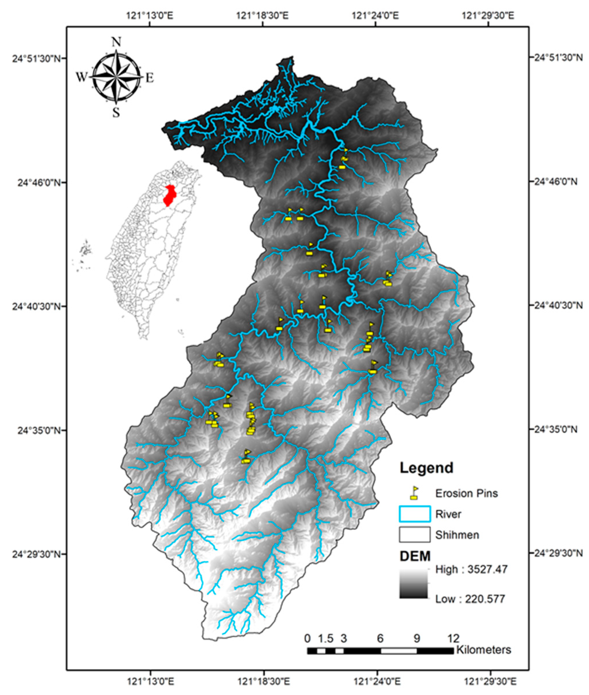
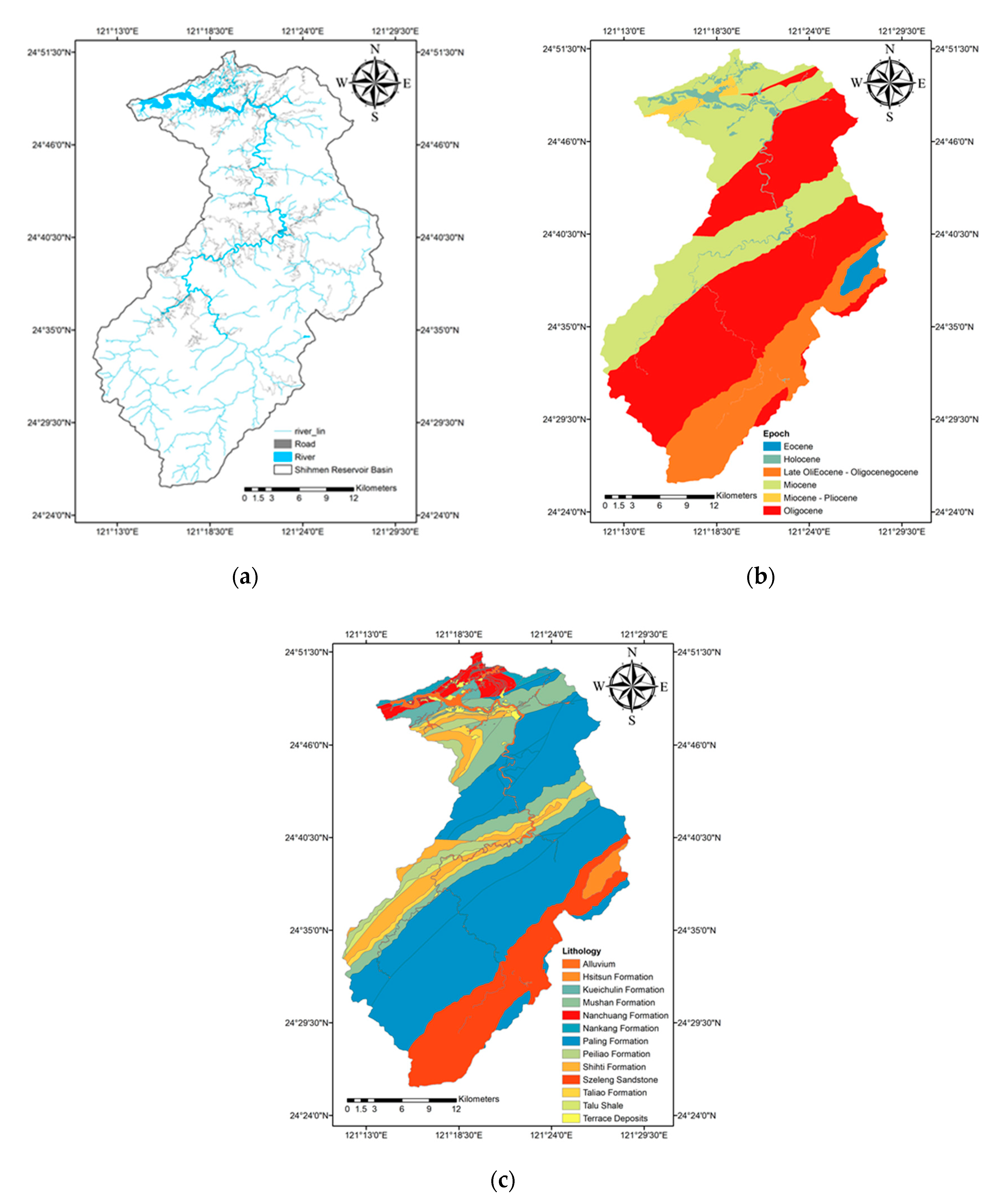
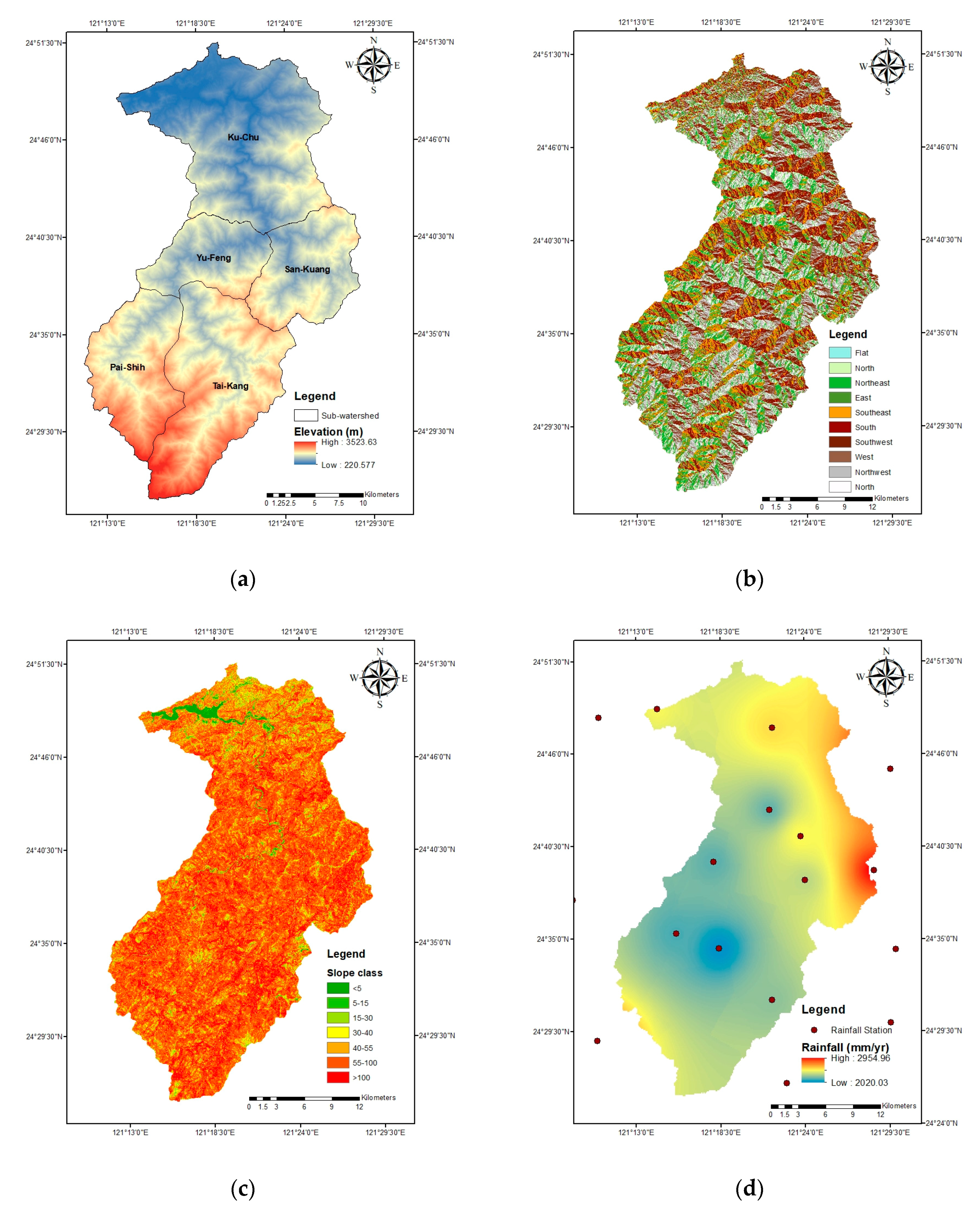
2.1. Study Area
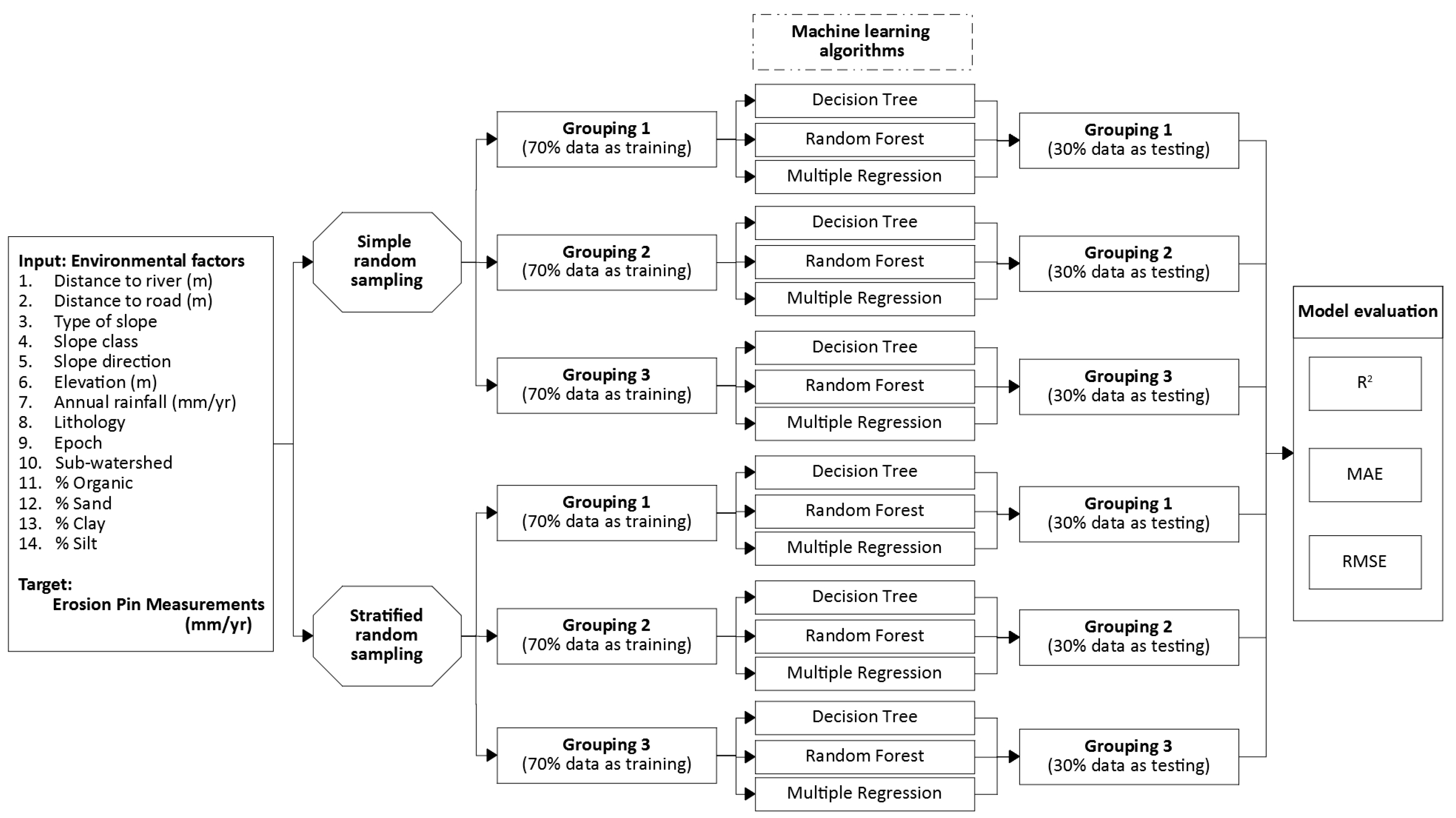
2.2. Research Framework
2.3. Data Collection
2.3.1. Erosion Pin Measurements
2.3.2. Environmental Factors
2.4. Data Separation
2.5. Model Construction
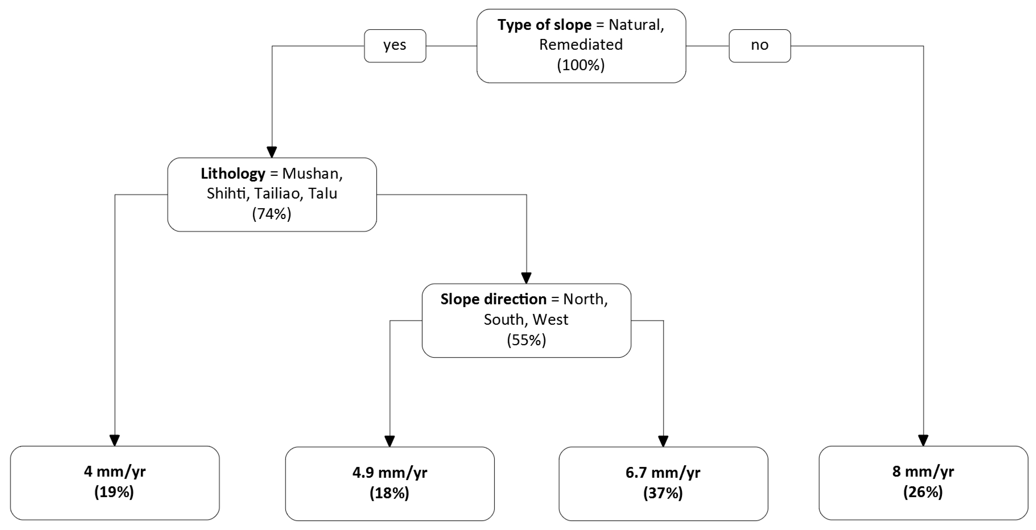
2.5.1. Decision Tree
2.5.2. Random Forest
2.5.3. Multiple Regression
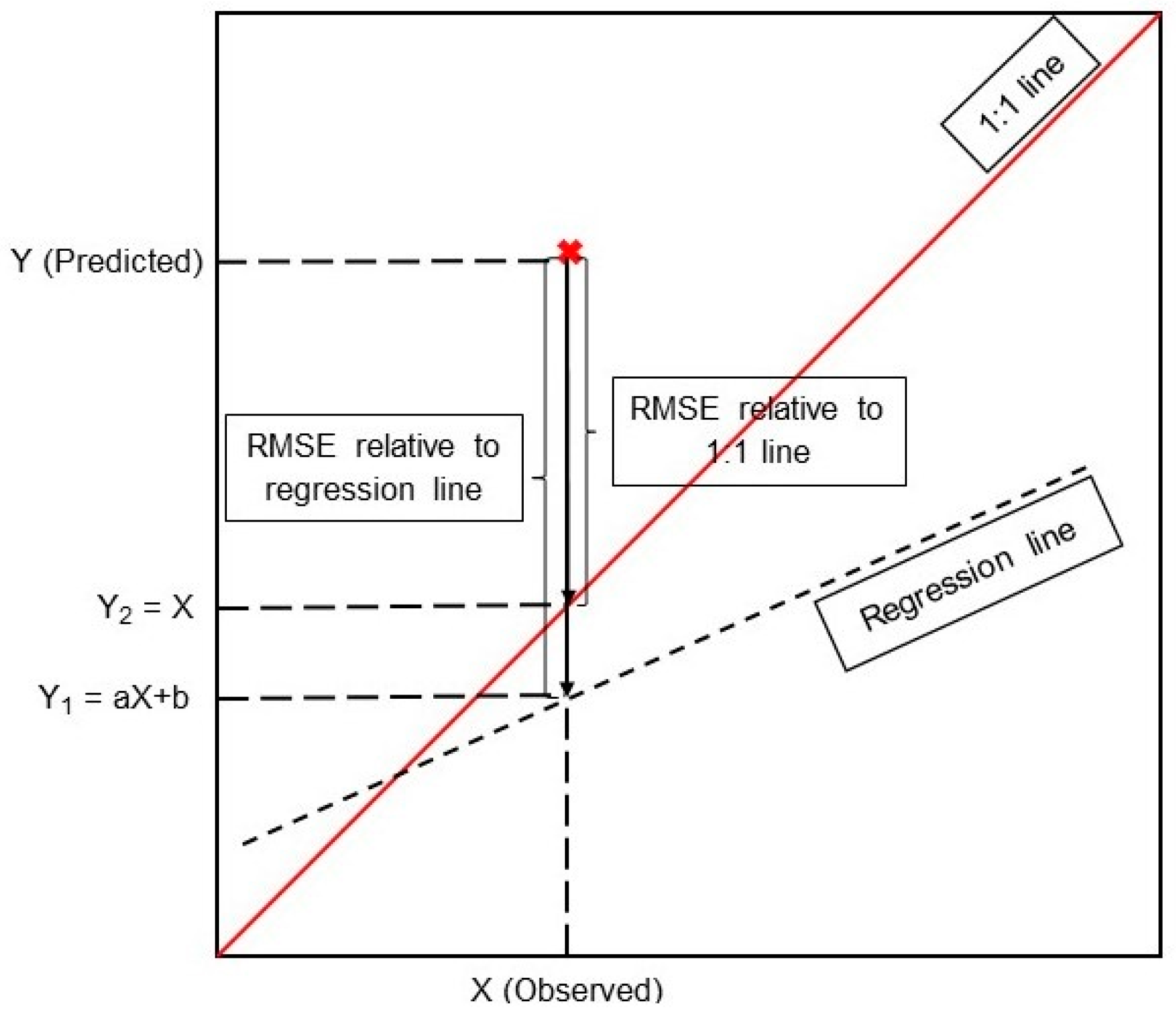
2.6. Model Performance Evaluation
3. Results and Discussion
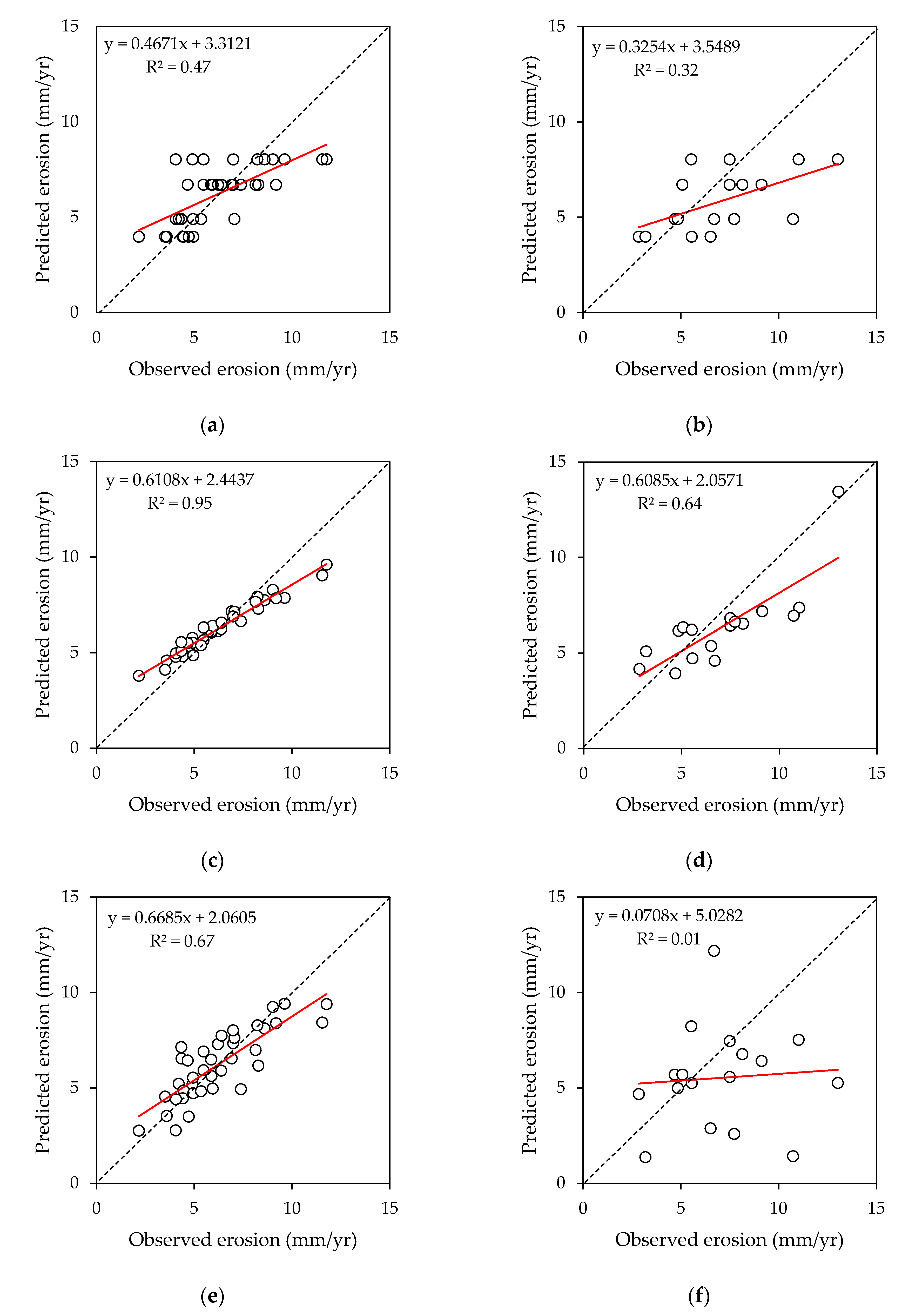
3.1. Comparison between Machine Learning Models and Multiple Regression
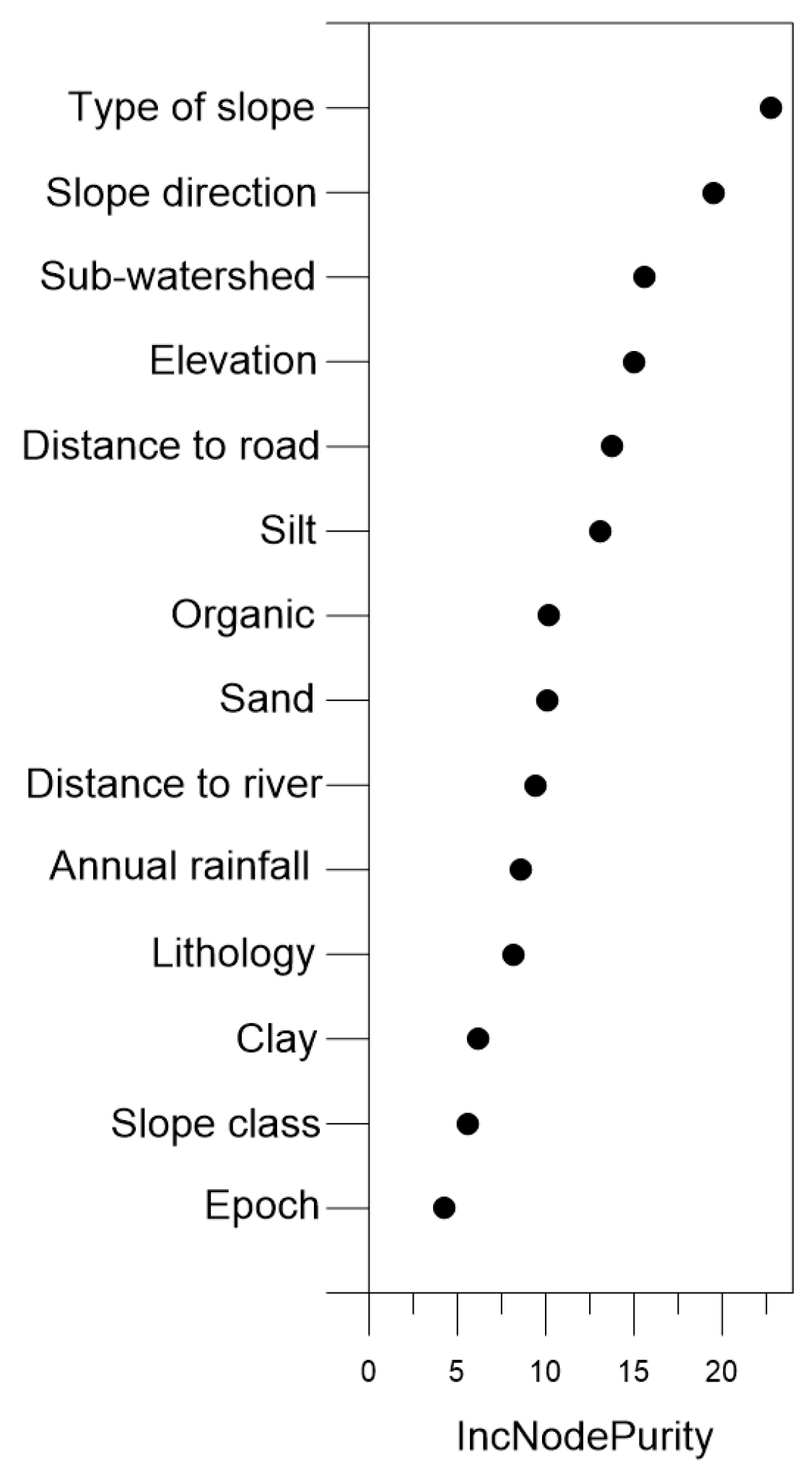
3.2. Identification of Important Factors
3.3. Comparison between Machine Learning Models and Traditional Soil Erosion Models
4. Conclusions
Author Contributions
Funding
Acknowledgments
Conflicts of Interest
References
- Amore, E.; Modica, C.; Nearing, M.A.; Santoro, V.C. Scale effect in USLE and WEPP application for soil erosion computation from three Sicilian basins. J. Hydrol. 2004, 293, 100–114. [Google Scholar] [CrossRef]
- Islam, M.R.; Jaafar, W.Z.W.; Hin, L.S.; Osman, N.; Hossain, A.; Mohd, N.S. Development of an intelligent system based on ANFIS model for predicting soil erosion. Environ. Earth Sci. 2018, 77, 186. [Google Scholar] [CrossRef]
- Tsai, Z.-X.; You, G.J.Y.; Lee, H.-Y.; Chiu, Y.-J. Use of a total station to monitor post-failure sediment yields in landslide sites of the Shihmen reservoir watershed, Taiwan. Geomorphology 2012, 139, 438–451. [Google Scholar] [CrossRef]
- Chen, Y.-J.; Chang, K.-C. A spatial–temporal analysis of impacts from human development on the Shih-men Reservoir watershed, Taiwan. Int. J. Remote Sens. 2011, 32, 9473–9496. [Google Scholar] [CrossRef]
- Chen, W.; Li, D.-H.; Yang, K.-J.; Tsai, F.; Seeboonruang, U. Identifying and comparing relatively high soil erosion sites with four DEMs. Ecol. Eng. 2018, 120, 449–463. [Google Scholar] [CrossRef]
- Ghimire, S.K.; Higaki, D.; Bhattarai, T.P. Estimation of soil erosion rates and eroded sediment in a degraded catchment of the Siwalik Hills, Nepal. Land 2013, 2, 370–391. [Google Scholar] [CrossRef]
- Haigh, M.J. The use of erosion pins in the study of slope evolution. Br. Geomorphol. Res. Group Tech. Bull. 1977, 18, 31–49. [Google Scholar]
- Edeso, J.; Merino, A.; Gonzalez, M.; Marauri, P. Soil erosion under different harvesting managements in steep forestlands from northern Spain. Land Degrad. Dev. 1999, 10, 79–88. [Google Scholar] [CrossRef]
- Saynor, M.J.; Loughran, R.J.; Erskine, W.D.; Scott, P. Sediment movement on hillslopes measured by caesium-137 and erosion pins. In Variability in Stream Erosion and Sediment Transport, Proceedings of the Canberra Symposium; No. 224; IAHS Publ.: Wallingford, UK, 1994; pp. 87–93. [Google Scholar]
- Lin, B.S.; Thomas, K.; Chen, C.K.; Ho, H.C. Evaluation of soil erosion risk for watershed management in Shenmu watershed, central Taiwan using USLE model parameters. Paddy Water Environ. 2016, 14, 19–43. [Google Scholar] [CrossRef]
- Liu, Y.-H.; Li, D.-H.; Chen, W.; Lin, B.-S.; Seeboonruang, U.; Tsai, F. Soil erosion modeling and comparison using slope units and grid cells in Shihmen reservoir watershed in northern Taiwan. Water 2018, 10, 1387. [Google Scholar] [CrossRef]
- Chen, W.; Chen, A. A statistical test of erosion pin measurements. In Proceedings of the 39th Asian Conference on Remote Sensing (ACRS 2018), Kuala Lumpur, Malaysia, 15–19 October 2018. [Google Scholar]
- Youssef, A.M.; Pourghasemi, H.R.; Pourtaghi, Z.S.; Al-Katheeri, M.M. Landslide susceptibility mapping using random forest, boosted regression tree, classification and regression tree, and general linear models and comparison of their performance at Wadi Tayyah Basin, Asir Region, Saudi Arabia. Landslides 2016, 13, 839–856. [Google Scholar] [CrossRef]
- Chen, W.; Panahi, M.; Pourghasemi, H.R. Performance evaluation of GIS-based new ensemble data mining techniques of adaptive neuro-fuzzy inference system (ANFIS) with genetic algorithm (GA), differential evolution (DE), and particle swarm optimization (PSO) for landslide spatial modelling. Catena 2017, 157, 310–324. [Google Scholar] [CrossRef]
- Kuhnert, P.M.; Henderson, A.K.; Bartley, R.; Herr, A. Incorporating uncertainty in gully erosion calculations using the random forests modelling approach. Environmetrics 2010, 21, 493–509. [Google Scholar] [CrossRef]
- Kheir, R.B.; Chorowicz, J.; Abdallah, C.; Dhont, D. Soil and bedrock distribution estimated from gully form and frequency: A GIS-based decision-tree model for Lebanon. Geomorphology 2008, 93, 482–492. [Google Scholar] [CrossRef]
- Tsai, F.; Lai, J.-S.; Chen, W.W.; Lin, T.-H. Analysis of topographic and vegetative factors with data mining for landslide verification. Ecol. Eng. 2013, 61, 669–677. [Google Scholar] [CrossRef]
- Liu, B.; Nearing, M.; Shi, P.; Jia, Z. Slope length effects on soil loss for steep slopes. Soil Sci. Soc. Am. J. 2000, 64, 1759–1763. [Google Scholar] [CrossRef]
- Liu, B.; Nearing, M.A.; Risse, L.M. Slope gradient effects on soil loss for steep slopes. Trans. ASAE 1994, 37, 1835–1840. [Google Scholar] [CrossRef]
- Lin, B.-S.; Chen, C.-K.; Thomas, K.; Hsu, C.-K.; Ho, H.-C. Improvement of the K-factor of USLE and soil erosion estimation in Shihmen reservoir watershed. Sustainability 2019, 11, 355. [Google Scholar] [CrossRef]
- Hong, H.; Panahi, M.; Shirzadi, A.; Ma, T.; Liu, J.; Zhu, A.X.; Kazakis, N. Flood susceptibility assessment in Hengfeng area coupling adaptive neuro-fuzzy inference system with genetic algorithm and differential evolution. Sci. Total Environ. 2018, 621, 1124–1141. [Google Scholar] [CrossRef]
- Lee, S.; Kim, Y.-S.; Oh, H.-J. Application of a weights-of-evidence method and GIS to regional groundwater productivity potential mapping. J. Environ. Manag. 2012, 96, 91–105. [Google Scholar] [CrossRef] [PubMed]
- Riaz, M.T.; Basharat, M.; Hameed, N.; Shafique, M.; Luo, J. A data-driven approach to landslide-susceptibility mapping in mountainous terrain: case study from the Northwest Himalayas, Pakistan. Nat. Hazards Rev. 2018, 19, 05018007. [Google Scholar] [CrossRef]
- Lantz, B. Machine Learning with R; Packt Publishing Ltd.: Birmingham, UK, 2013. [Google Scholar]
- Breiman, L. Random forests. Mach. Learn. 2001, 45, 5–32. [Google Scholar] [CrossRef]
- Micheletti, N.; Foresti, L.; Robert, S.; Leuenberger, M.; Pedrazzini, A.; Jaboyedoff, M.; Kanevski, M. Machine learning feature selection methods for landslide susceptibility mapping. Math. Geosci. 2014, 46, 33–57. [Google Scholar] [CrossRef]
- Prasad, A.M.; Iverson, L.R.; Liaw, A. Newer classification and regression tree techniques: Bagging and random forests for ecological prediction. Ecosystems 2006, 9, 181–199. [Google Scholar] [CrossRef]
- Arnaez, J.; Lasanta, T.; Ruiz-Flaño, P.; Ortigosa, L. Factors affecting runoff and erosion under simulated rainfall in Mediterranean vineyards. Soil Tillage Res. 2007, 93, 324–334. [Google Scholar] [CrossRef]
- Bagio, B.; Bertol, I.; Wolschick, N.H.; Schneiders, D.; dos Santos, M.A.N. Water erosion in different slope lengths on bare soil. Revista Brasileira de Ciência do Solo 2017, 41. [Google Scholar] [CrossRef]
- Zhang, W.; Zhou, J.; Feng, G.; Weindorf, D.C.; Hu, G.; Sheng, J. Characteristics of water erosion and conservation practice in arid regions of Central Asia: Xinjiang Province, China as an example. Int. Soil Water Conserv. Res. 2015, 3, 97–111. [Google Scholar] [CrossRef]


| Simple Random Sampling | Decision Tree | Random Forest | Multiple Regression | |||||||||
|---|---|---|---|---|---|---|---|---|---|---|---|---|
| Training | Testing | Training | Testing | Training | Testing | |||||||
| Grouping #1 | 1:1 | Reg. | 1:1 | Reg. | 1:1 | Reg. | 1:1 | Reg. | 1:1 | Reg. | 1:1 | Reg. |
| MAE (mm/yr) | 1.42 | 0.94 | 1.72 | 1.25 | 0.79 | 0.31 | 1.33 | 0.35 | 1.21 | 0.94 | 1.48 | 1.21 |
| RMSE (mm/yr) | 1.76 | 1.25 | 2.16 | 1.39 | 0.95 | 0.41 | 1.70 | 0.48 | 1.47 | 1.19 | 1.81 | 1.47 |
| R2 | - | 0.50 * | - | 0.05 | - | 0.94 * | - | 0.38 * | - | 0.65 * | - | 0.31 |
| Grouping #2 | 1:1 | Reg. | 1:1 | Reg. | 1:1 | Reg. | 1:1 | Reg. | 1:1 | Reg. | 1:1 | Reg. |
| MAE (mm/yr) | 1.38 | 0.92 | 2.15 | 1.02 | 0.79 | 0.28 | 1.59 | 0.42 | 1.22 | 0.88 | 2.03 | 1.57 |
| RMSE (mm/yr) | 1.75 | 1.16 | 2.55 | 1.31 | 0.99 | 0.38 | 1.78 | 0.57 | 1.43 | 1.13 | 2.33 | 1.84 |
| R2 | - | 0.44 | - | 0.12 | - | 0.94 * | - | 0.64 * | - | 0.63 * | - | 0.33 |
| Grouping #3 | 1:1 | Reg. | 1:1 | Reg. | 1:1 | Reg. | 1:1 | Reg. | 1:1 | Reg. | 1:1 | Reg. |
| MAE (mm/yr) | 1.37 | 1.04 | 2.32 | 1.61 | 0.73 | 0.30 | 1.61 | 0.60 | 1.16 | 0.89 | 1.83 | 1.28 |
| RMSE (mm/yr) | 1.80 | 1.22 | 2.66 | 1.66 | 0.93 | 0.37 | 1.81 | 0.85 | 1.43 | 1.16 | 2.16 | 1.68 |
| R2 | - | 0.46 * | - | 0.01 | - | 0.95 * | - | 0.33 | - | 0.66 * | - | 0.12 |
| Average | 1:1 | Reg. | 1:1 | Reg. | 1:1 | Reg. | 1:1 | Reg. | 1:1 | Reg. | 1:1 | Reg. |
| MAE (mm/yr) | 1.39 | 0.97 | 2.06 | 1.29 | 0.77 | 0.30 | 1.51 | 0.46 | 1.20 | 0.90 | 1.78 | 1.35 |
| RMSE (mm/yr) | 1.77 | 1.21 | 2.46 | 1.45 | 0.96 | 0.39 | 1.76 | 0.63 | 1.44 | 1.16 | 2.10 | 1.66 |
| R2 | - | 0.47 * | - | 0.06 | - | 0.94 * | - | 0.45 * | - | 0.65 * | - | 0.25 |
| Stratified Random Sampling | Decision Tree | Random Forest | Multiple Regression | |||||||||
|---|---|---|---|---|---|---|---|---|---|---|---|---|
| Training | Testing | Training | Testing | Training | Testing | |||||||
| Grouping #1 | 1:1 | Reg. | 1:1 | Reg. | 1:1 | Reg. | 1:1 | Reg. | 1:1 | Reg. | 1:1 | Reg. |
| MAE (mm/yr) | 1.63 | 0.83 | 1.87 | 0.96 | 0.76 | 0.24 | 1.44 | 0.84 | 0.95 | 0.77 | 2.51 | 2.33 |
| RMSE (mm/yr) | 2.00 | 0.93 | 2.53 | 1.01 | 0.93 | 0.30 | 1.68 | 1.06 | 1.22 | 1.03 | 3.19 | 2.97 |
| R2 | - | 0.22 | - | 0.08 | - | 0.95 * | - | 0.59 * | - | 0.71 * | - | 0.19 |
| Grouping #2 | 1:1 | Reg. | 1:1 | Reg. | 1:1 | Reg. | 1:1 | Reg. | 1:1 | Reg. | 1:1 | Reg. |
| MAE (mm/yr) | 1.19 | 0.87 | 2.01 | 1.03 | 0.68 | 0.24 | 1.51 | 0.97 | 0.95 | 0.84 | 2.90 | 1.84 |
| RMSE (mm/yr) | 1.58 | 1.08 | 2.52 | 1.27 | 0.89 | 0.29 | 1.77 | 1.24 | 1.25 | 1.02 | 3.89 | 2.57 |
| R2 | - | 0.47 * | - | 0.32 | - | 0.95 * | - | 0.64 * | - | 0.67 * | - | 0.01 |
| Grouping #3 | 1:1 | Reg. | 1:1 | Reg. | 1:1 | Reg. | 1:1 | Reg. | 1:1 | Reg. | 1:1 | Reg. |
| MAE (mm/yr) | 1.27 | 0.90 | 1.73 | 1.31 | 0.78 | 0.25 | 1.36 | 0.64 | 1.13 | 0.91 | 2.26 | 2.01 |
| RMSE (mm/yr) | 1.61 | 1.16 | 2.31 | 1.49 | 0.97 | 0.35 | 1.79 | 0.82 | 1.29 | 1.07 | 3.33 | 2.97 |
| R2 | - | 0.52 * | - | 0.18 | - | 0.94 * | - | 0.51 * | - | 0.69 * | - | 0.14 |
| Average | 1:1 | Reg. | 1:1 | Reg. | 1:1 | Reg. | 1:1 | Reg. | 1:1 | Reg. | 1:1 | Reg. |
| MAE (mm/yr) | 1.36 | 0.87 | 1.87 | 1.10 | 0.74 | 0.24 | 1.44 | 0.82 | 1.01 | 0.84 | 2.56 | 2.06 |
| RMSE (mm/yr) | 1.73 | 1.06 | 2.45 | 1.26 | 0.93 | 0.31 | 1.75 | 1.04 | 1.25 | 1.04 | 3.47 | 2.84 |
| R2 | - | 0.40 * | - | 0.19 | - | 0.95 * | - | 0.58 * | - | 0.69 * | 0.11 | |
| Bare | Natural | Remediated | |
|---|---|---|---|
| Number of pins | 14 | 21 | 20 |
| Average (mm/yr) | 8.38 | 6.42 | 5.19 |
| Important Findings | |
|---|---|
| Finding #1 | When an insufficient amount of site-specific data is available to apply an empirically or physically based soil erosion model, machine learning-based approaches are shown to provide an alternative method to analyze data from different slopes and predict soil erosion depths in a watershed. |
| Finging #2 | To predict the soil erosion depths of the Shihmen reservoir watershed in Taiwan, the stratified random sampling method is proved to yield better results than the simple random sampling method. |
| Finding #3 | When decision tree and random forest algorithms are compared with multiple regression analysis, the random forest algorithm performed the best of the three methods in the Shihmen reservoir watershed. |
| Finding #4 | The average error (as measured by RMSE) of the stratified random sampling method of the random forest algorithm is 0.93 mm/yr in the training data and 1.75 mm/yr in the testing data in the Shihmen reservoir watershed. |
© 2019 by the authors. Licensee MDPI, Basel, Switzerland. This article is an open access article distributed under the terms and conditions of the Creative Commons Attribution (CC BY) license (http://creativecommons.org/licenses/by/4.0/).
Share and Cite
Nguyen, K.A.; Chen, W.; Lin, B.-S.; Seeboonruang, U.; Thomas, K. Predicting Sheet and Rill Erosion of Shihmen Reservoir Watershed in Taiwan Using Machine Learning. Sustainability 2019, 11, 3615. https://doi.org/10.3390/su11133615
Nguyen KA, Chen W, Lin B-S, Seeboonruang U, Thomas K. Predicting Sheet and Rill Erosion of Shihmen Reservoir Watershed in Taiwan Using Machine Learning. Sustainability. 2019; 11(13):3615. https://doi.org/10.3390/su11133615
Chicago/Turabian StyleNguyen, Kieu Anh, Walter Chen, Bor-Shiun Lin, Uma Seeboonruang, and Kent Thomas. 2019. "Predicting Sheet and Rill Erosion of Shihmen Reservoir Watershed in Taiwan Using Machine Learning" Sustainability 11, no. 13: 3615. https://doi.org/10.3390/su11133615
APA StyleNguyen, K. A., Chen, W., Lin, B.-S., Seeboonruang, U., & Thomas, K. (2019). Predicting Sheet and Rill Erosion of Shihmen Reservoir Watershed in Taiwan Using Machine Learning. Sustainability, 11(13), 3615. https://doi.org/10.3390/su11133615