Realistic Traffic Condition Informed Life Cycle Assessment: Interstate 495 Maintenance and Rehabilitation Case Study


Abstract
:1. Introduction
2. Materials and Methods
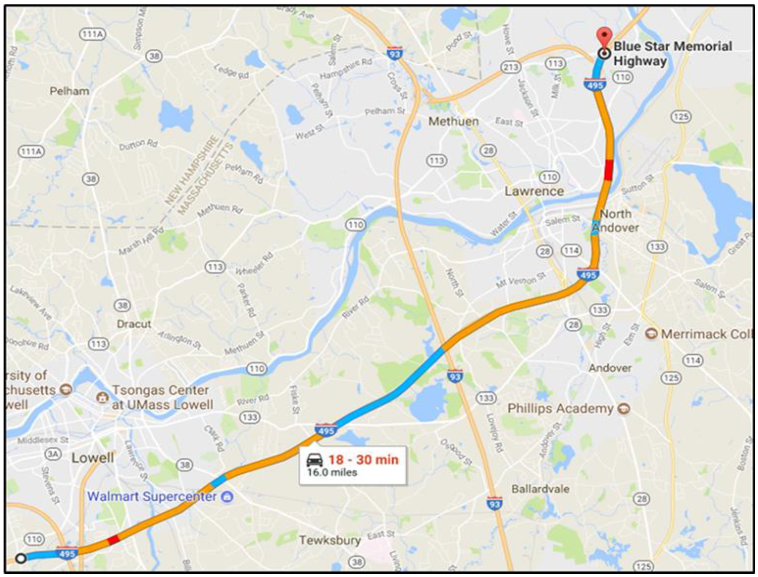
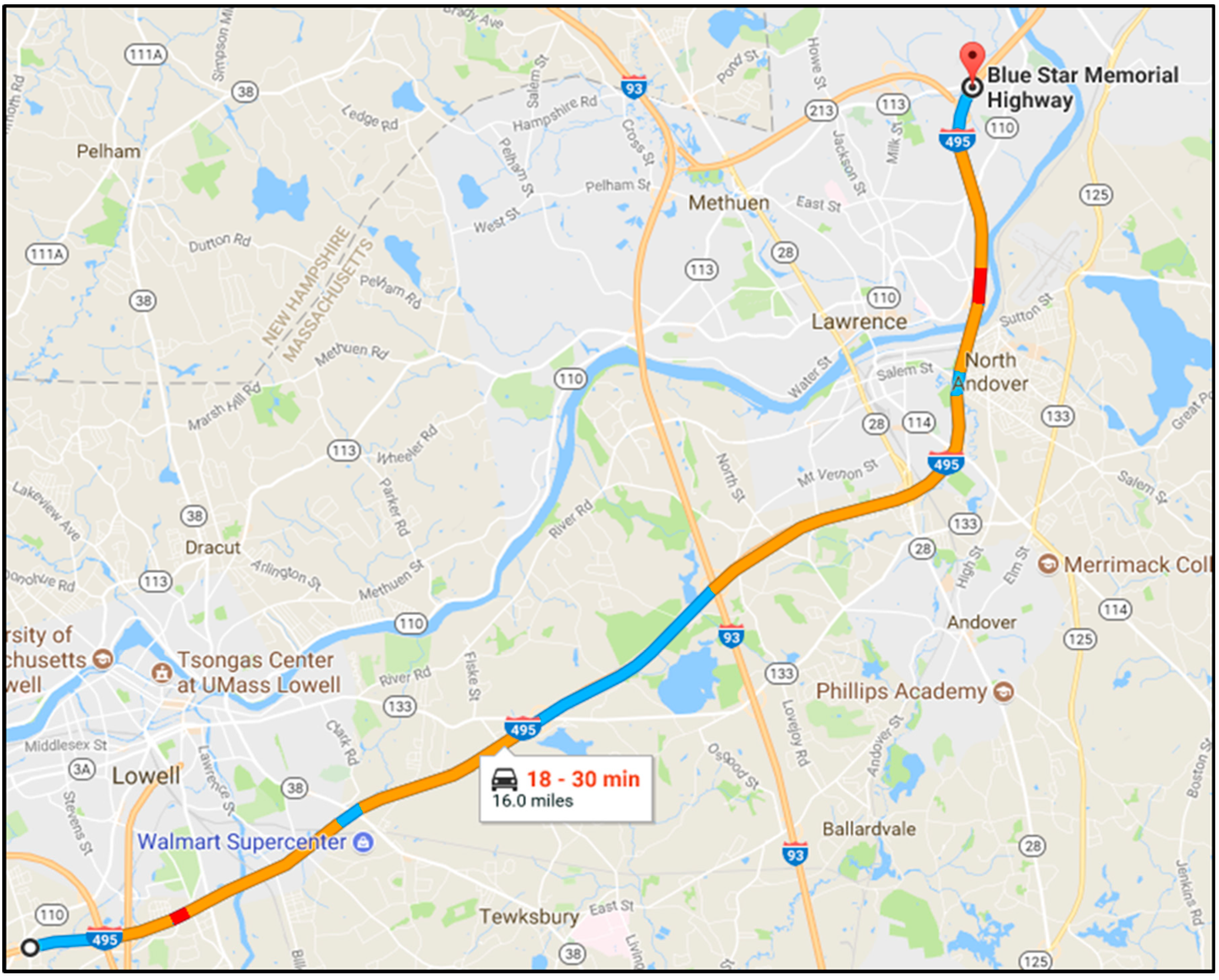
2.1. Case Study Location
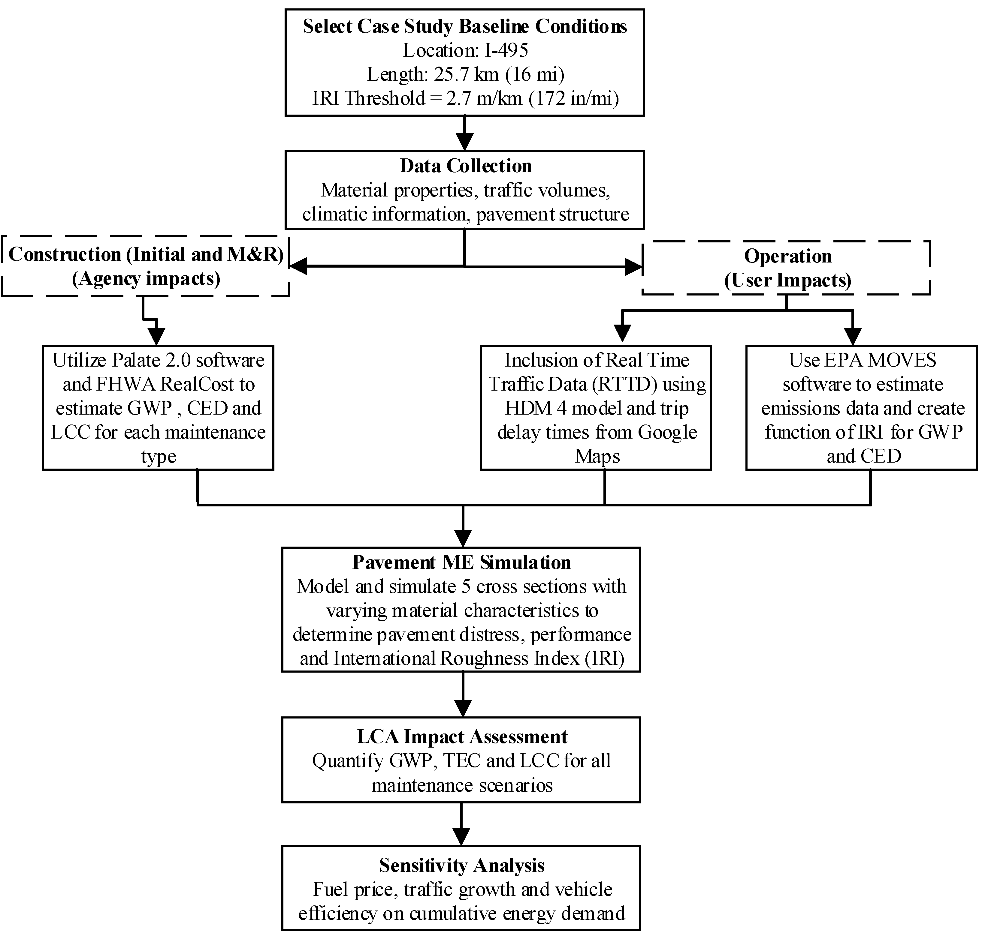
2.2. General Methodology
2.2.1. Construction Phase: Materials and Pavement Cross-Sections
2.2.2. Construction Phase: Maintenance and Rehabilitation
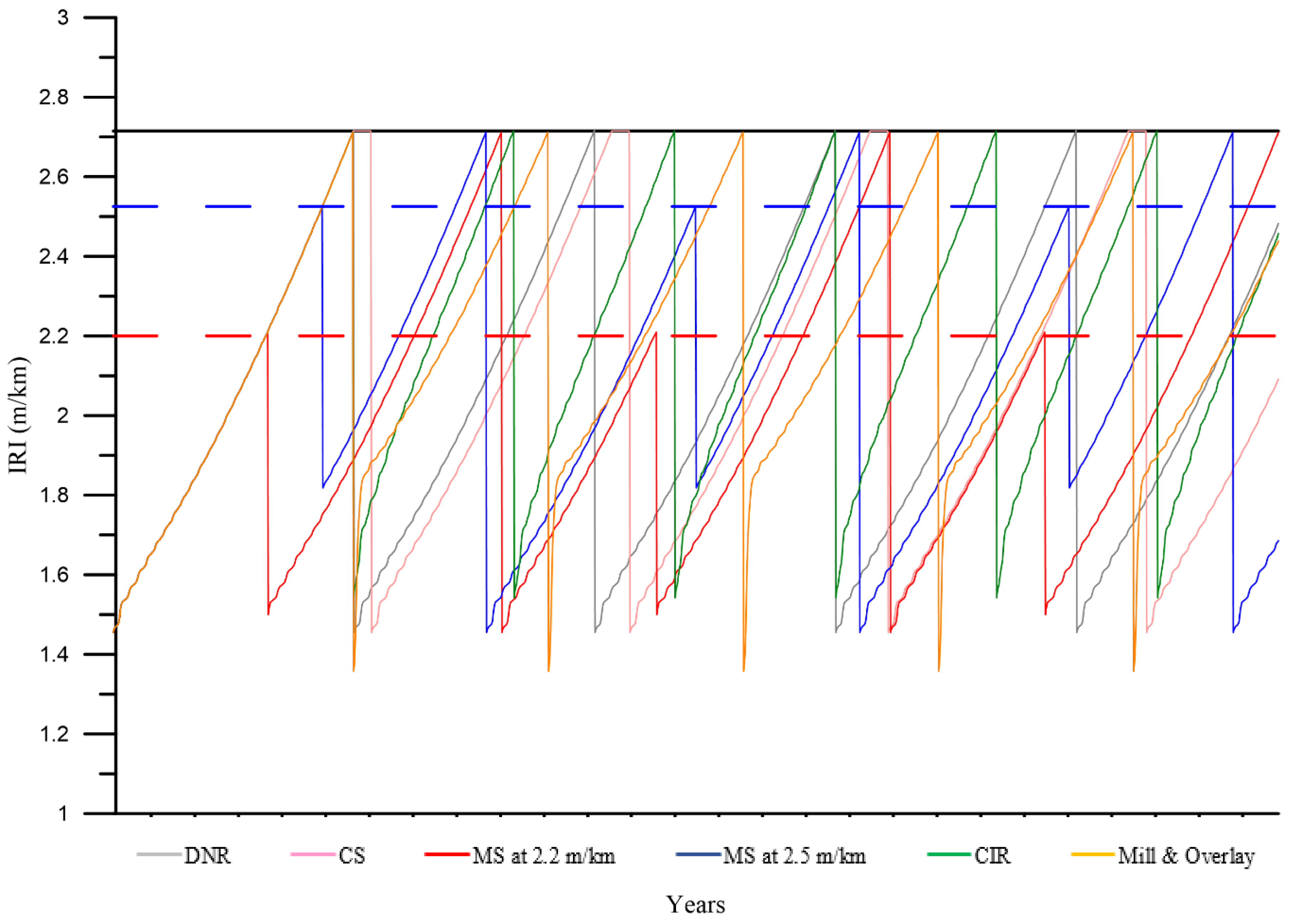
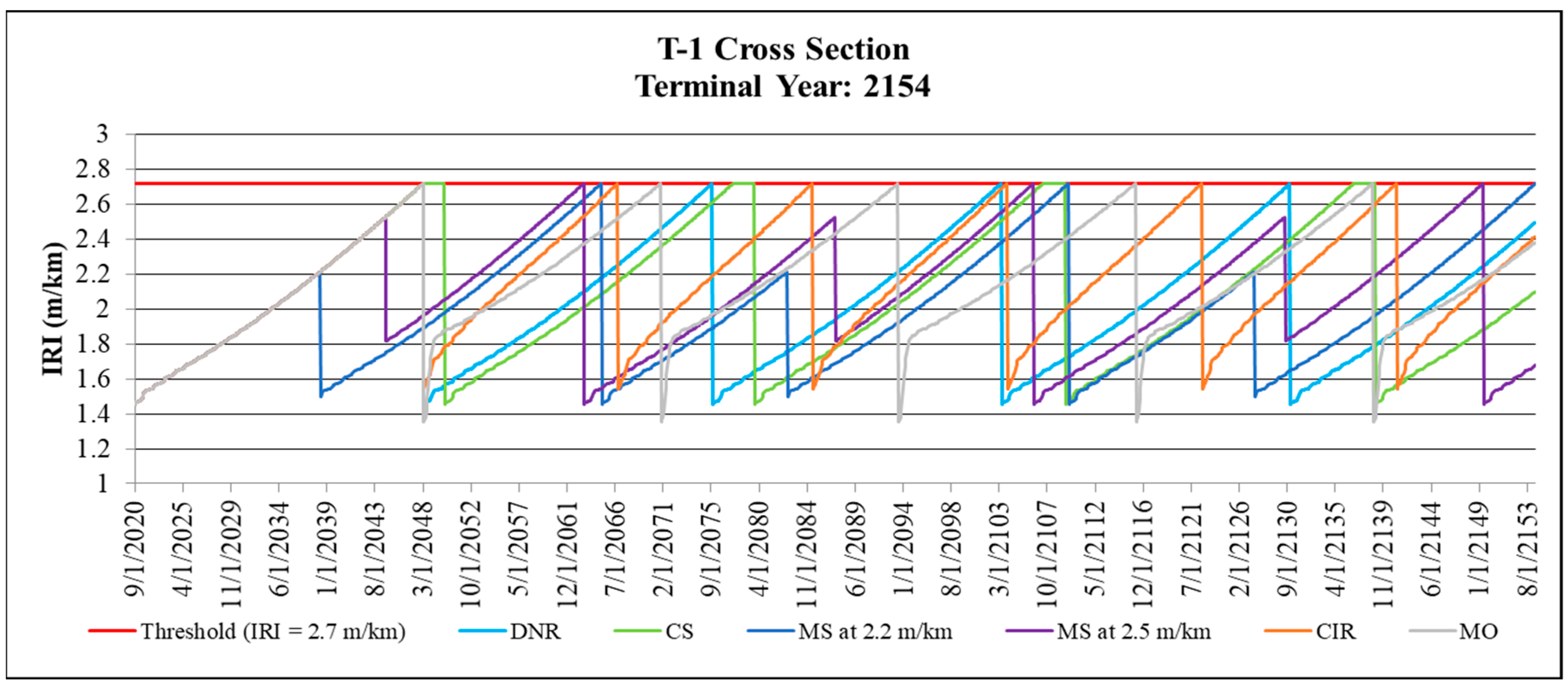
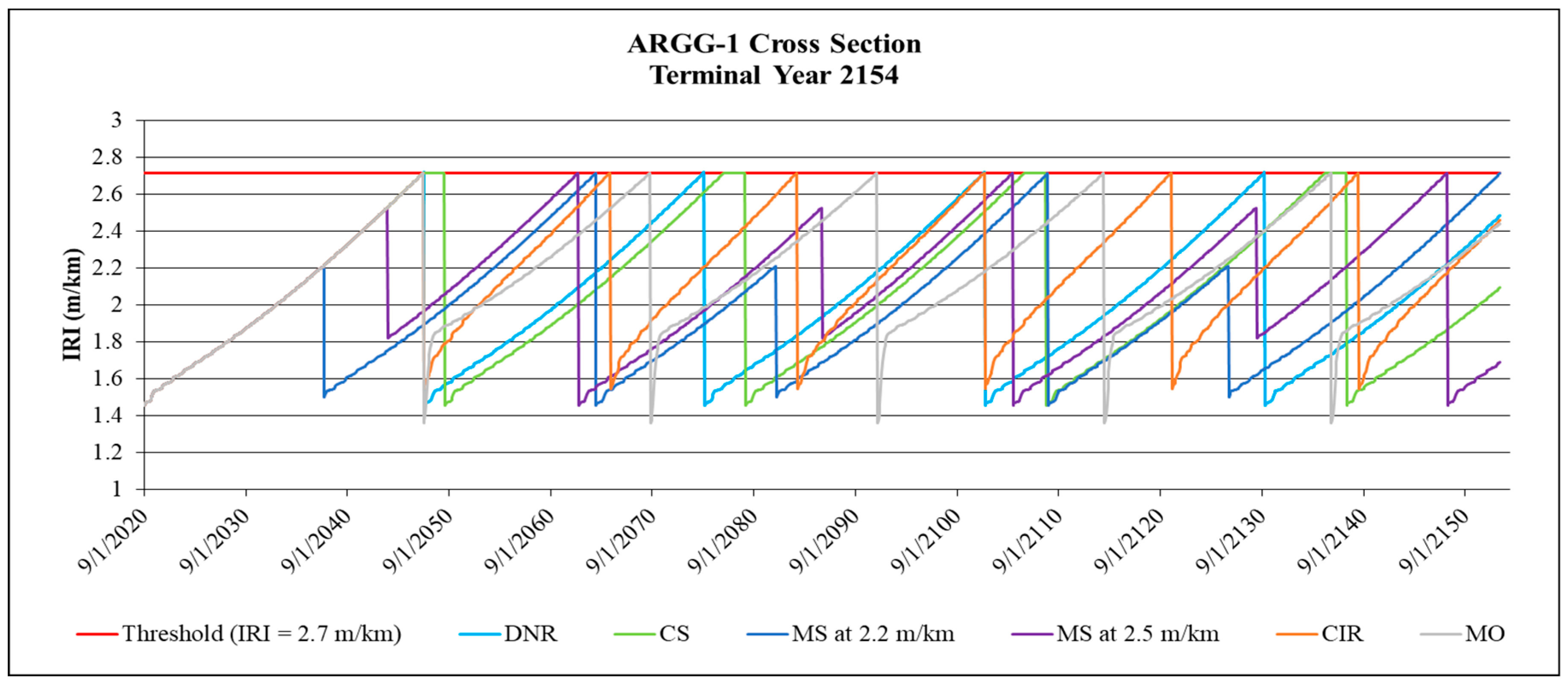
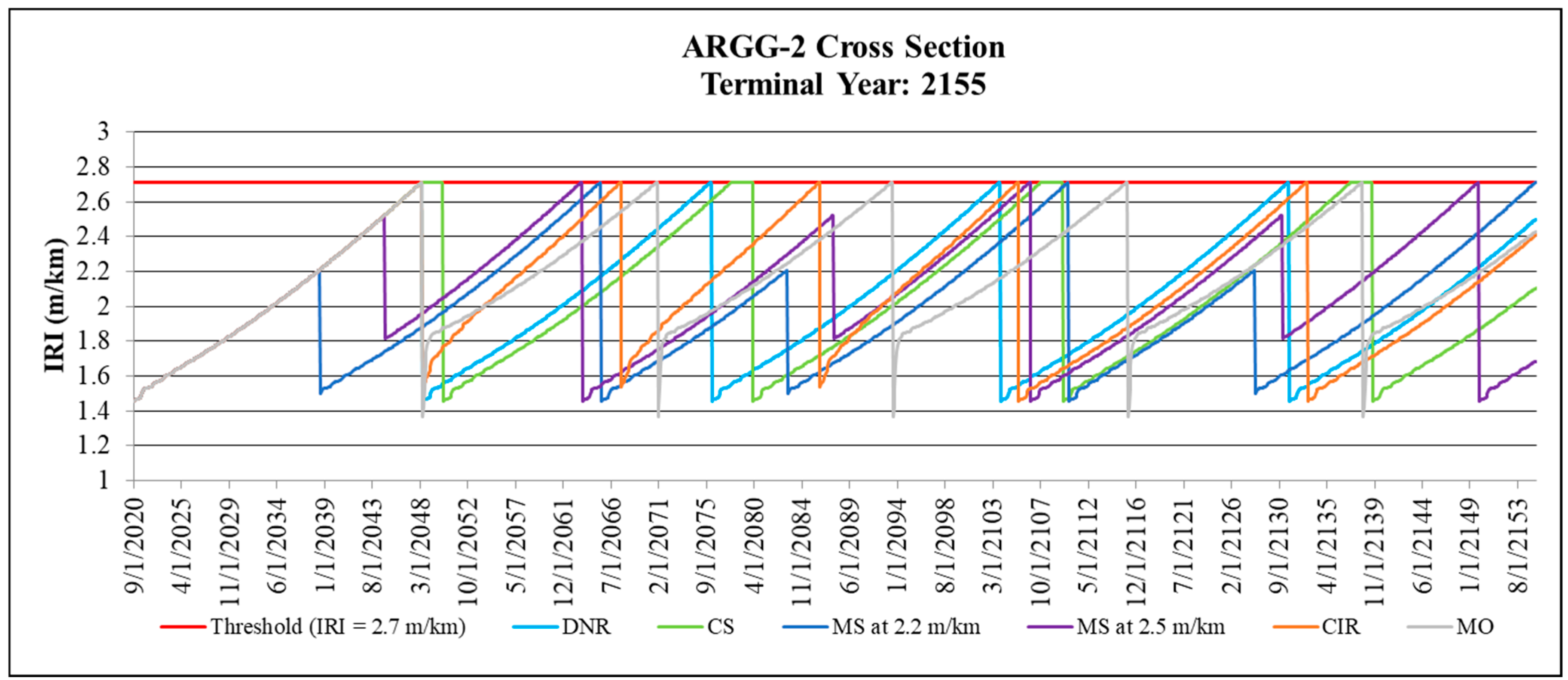
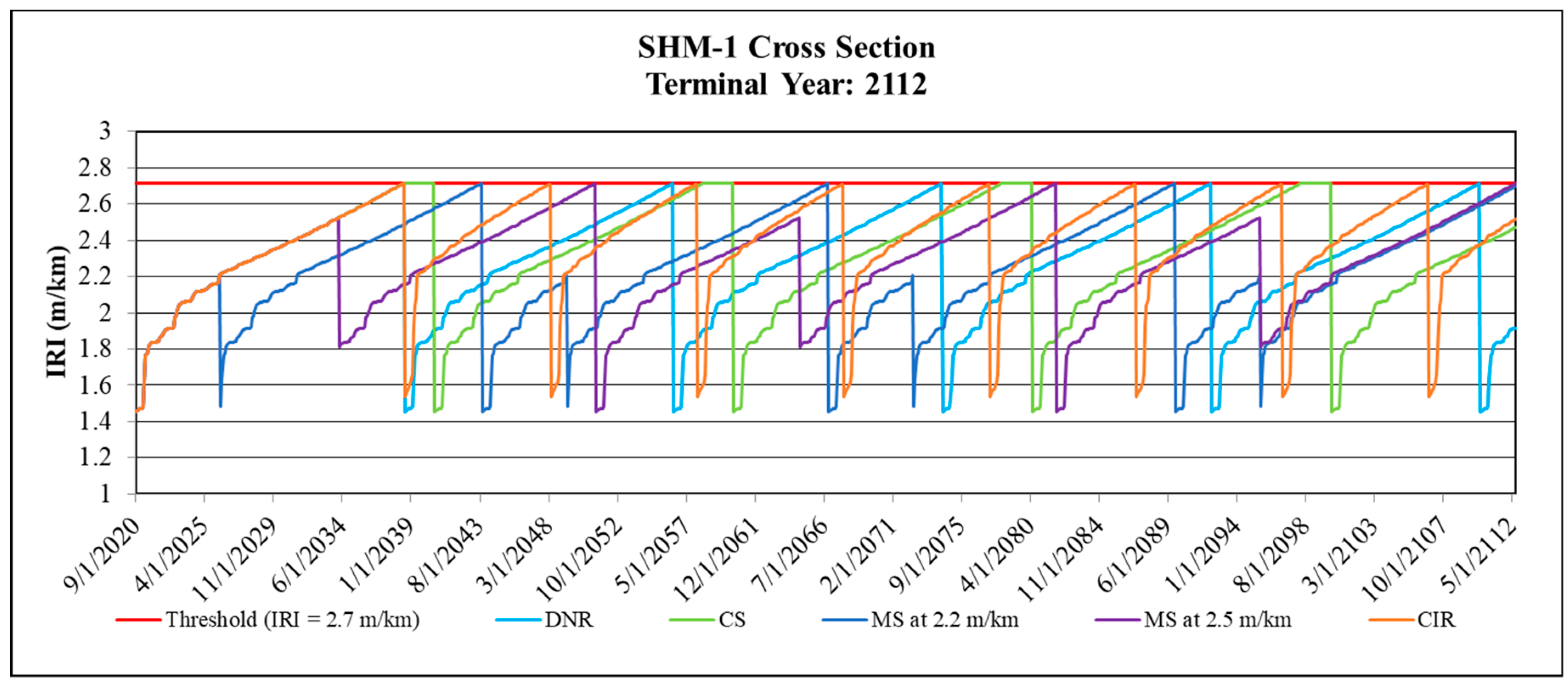
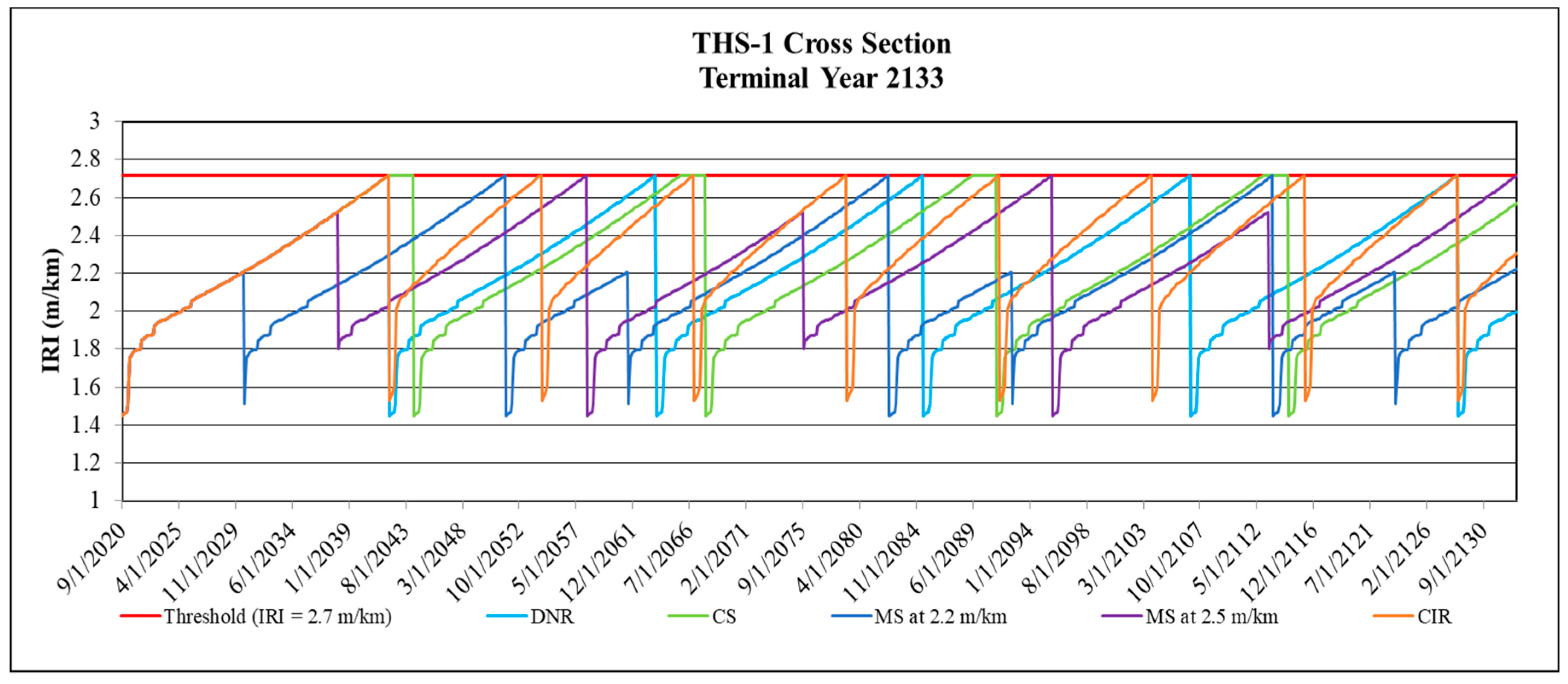
- Do nothing and reconstruct (DNR): The first M&R scenario is simply the choice to perform no maintenance or rehabilitation and to reconstruct at the end of the pavement system’s service life (reached the terminal IRI). The pavement performance curves in terms of IRI and time for this scenario are determined using Pavement ME.
- Crack sealant (CS): The next M&R alternative evaluated the use of a crack sealant every two years during the service life of the pavement until the terminal IRI value was reached and the pavement system was reconstructed. Crack sealant is a common preventative maintenance treatment to fill cracks at the surface of the pavement structure to prevent water from infiltrating. It was found in literature that the overall pavement service life is extended by 2 years when applying crack sealant as a pavement preservation technique [22]. For simplicity, it was assumed that the pavement continues to deteriorate at the same rate after applying the crack sealant treatment but a two-year extension of the service life was applied before reaching the terminal IRI trigger value. It should also be noted that crack sealant is a preservation treatment and does not address structural issues, as a M&R strategy does.
- Microsurfacing (MS 2.2 m/km): Microsurfacing was applied when an IRI trigger value of 2.2 m/km was reached. Microsurfacing is a common M&R treatment type that applies a mixture of water, asphalt emulsion, aggregate, and chemical additives to an existing asphalt pavement surface in order to preserve the underlying pavement structure. It provides a new pavement driving surface, and according to a study by MnDOT, it resets the IRI by approximately 0.7 m/km [23]. A type III microsurface was molded in this study. It should be highlighted that microsurfacing is a pavement preservation treatment and does not address underlying structural issues.
- Microsurfacing (MS 2.5 m/km): Microsurfacing was applied when an IRI trigger value of 2.5 m/km was reached. Once again, IRI was reset by approximately 0.7 m/km [23].
- Cold-In-Place (CIR) Recycling: CIR is a pavement rehabilitation technique that involves reclaiming 50 mm to 100 mm of the existing pavement structure. It is a similar process to cold plant mix recycling, except that it is performed directly in the field, typically by a paving train of equipment. Once the terminal IRI value has been triggered, the CIR treatment is performed and the IRI decreases by approximately 1.1 m/km [24,25]. The simulated cross-section after CIR was performed, consisting of a 5-cm asphalt concrete (AC) surface course, 5-cm AC base course, 10-cm of cold recycled asphalt pulverized in place, and 60-cm granular base. CIR is generally being accepted as a pavement rehabilitation strategy that has the ability to address structural distresses. Pavement ME was used to determine the pavement performance curves when CIR was used as a M&R strategy.
- Mill and Overlay (MO): Mill and overlay of approximately 50 mm was performed once the terminal IRI value was reached. On average, the IRI is reset by (0.95 to 1.26 m/km), therefore this M&R alternative scenario reset the IRI to the initial value of 1 m/km and then allowed the pavement cross-section to reach the terminal IRI value of 2.7 m/km before reconstruction [26,27]. Reconstruction was performed after one MO treatment to avoid the impractical scenario of constant MO highway pavement systems. MO often falls in the gray area as a mix between a surface treatment or a rehabilitation strategy. For the purpose of this study, MO is considered as a rehabilitation treatment capable of addressing structural distresses. Pavement ME simulations were conducted for each cross-section with use of MO treatment to determine the pavement performance curves.
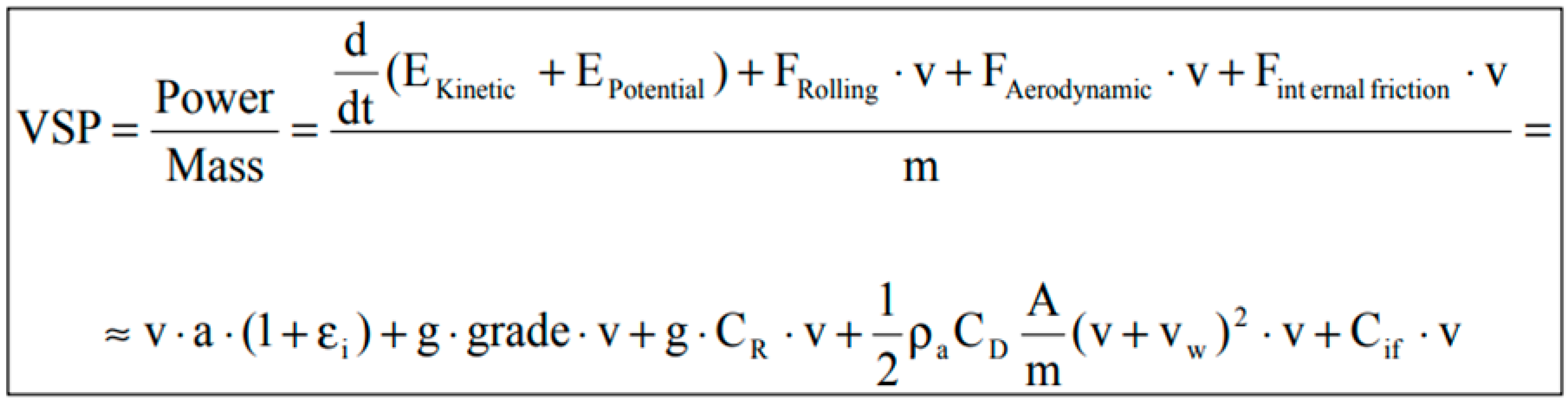
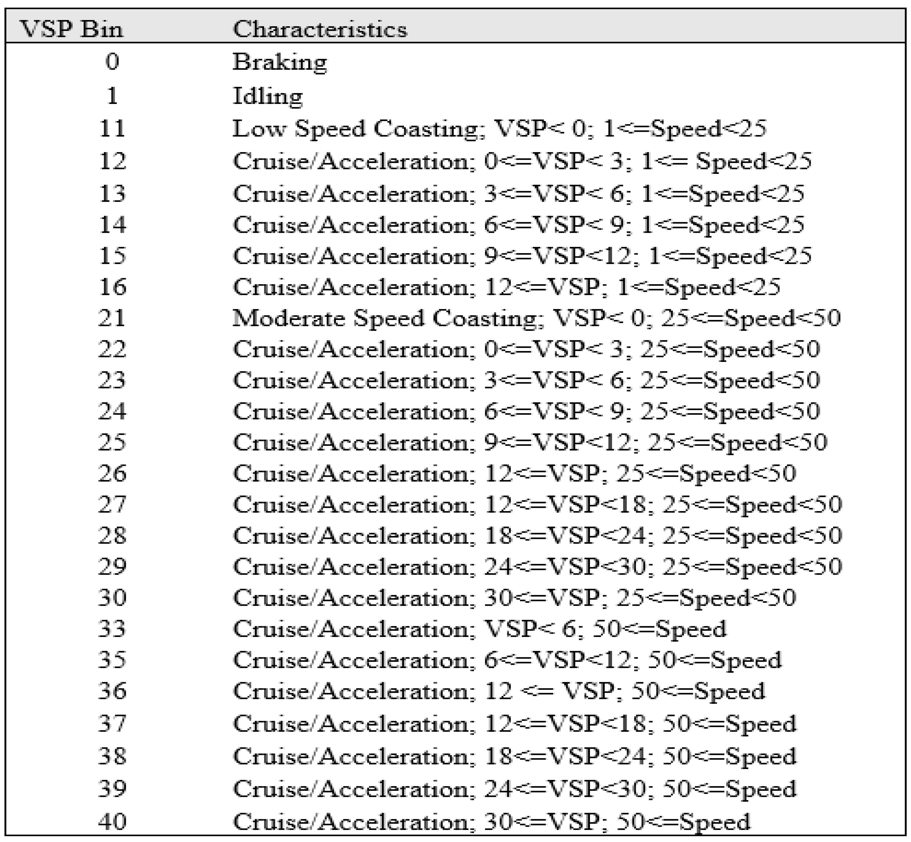
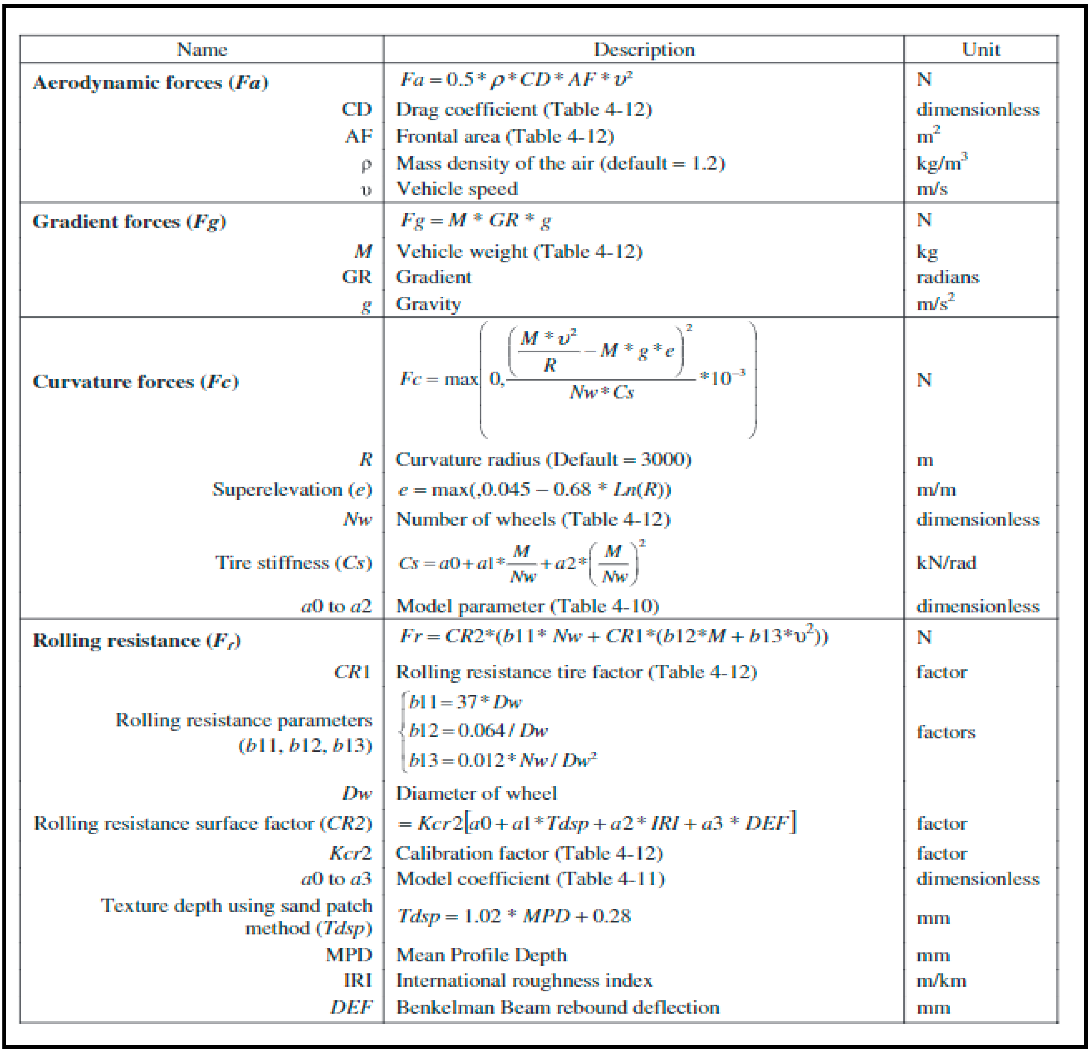
2.2.3. Use Phase
2.3. Life Cycle Cost Analysis
2.4. Sensitivity Analysis
3. Results
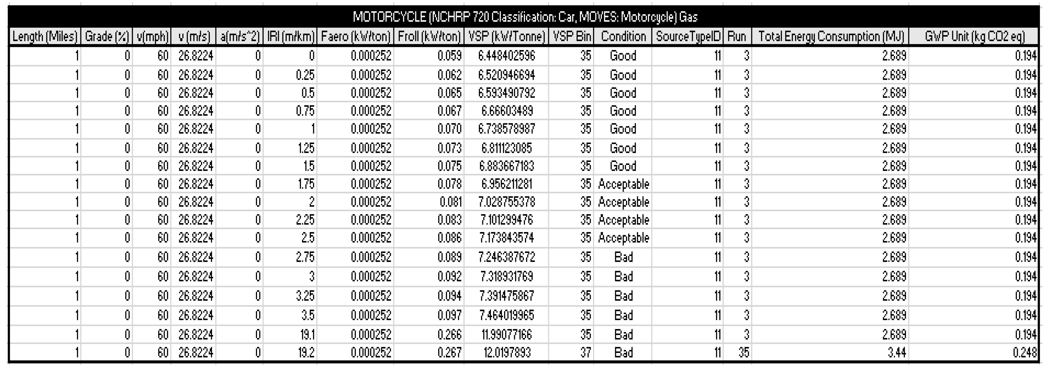
3.1. Effect of Realistic Traffic as Compared to Steady Speed
3.2. Overall LCA Results
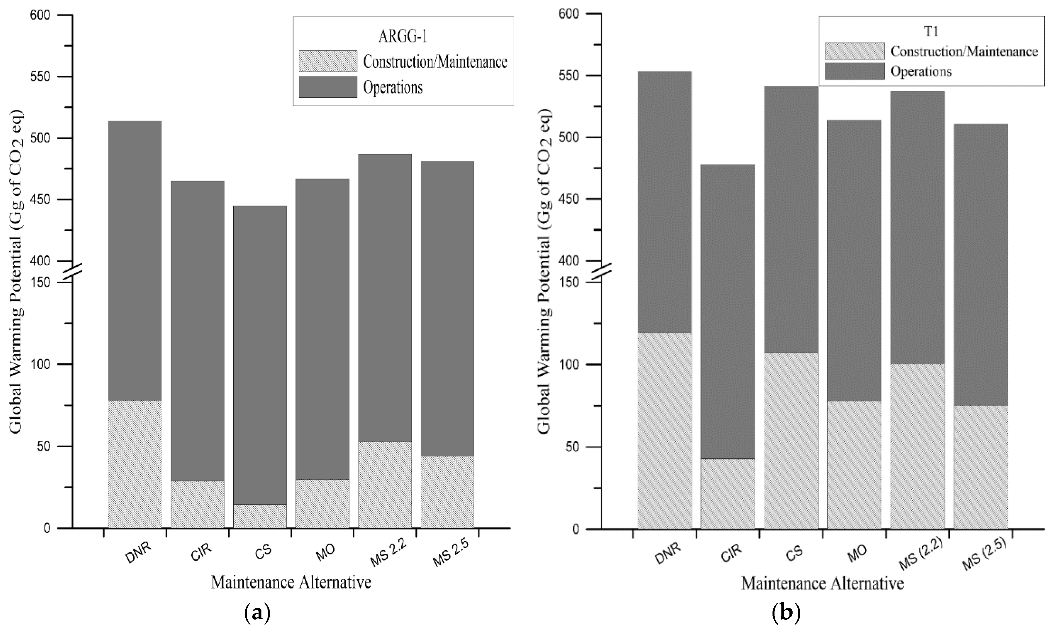
3.2.1. Global Warming Potential (GWP)
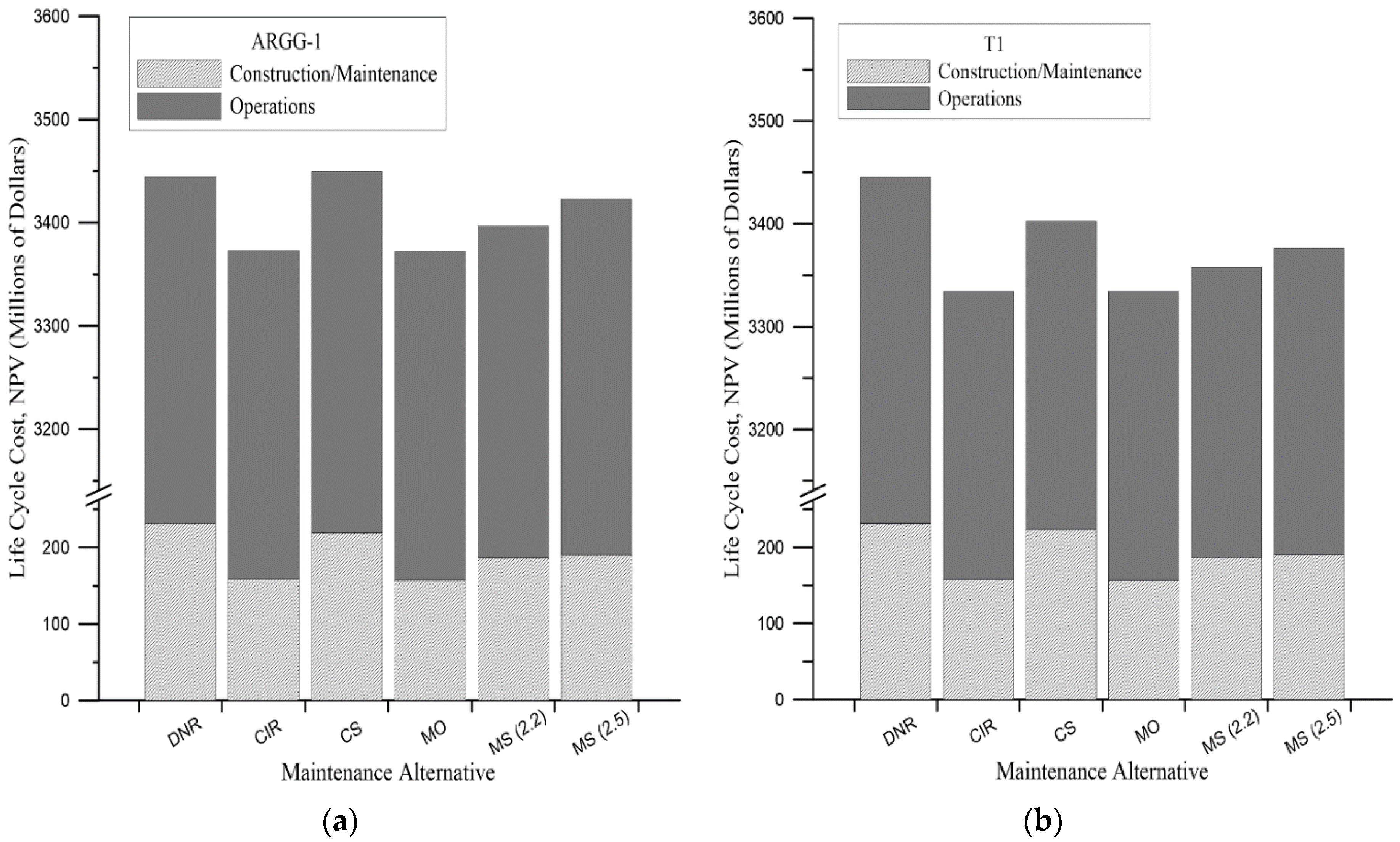
3.2.2. Life Cycle Cost (LCC)
3.3. Sensitivity Analysis
4. Discussion
5. Conclusions and Recommendations
Author Contributions
Funding
Acknowledgments
Conflicts of Interest
Appendix A
Appendix A.1. Life Cycle Inventory

| Impact Unit | Units | Value | Source |
|---|---|---|---|
| Production | |||
| Asphalt Concrete | MJ/ton | 641 | SimaPro |
| Asphalt Concrete | kg CO2 eq/ton | 84.7 | SimaPro |
| Gravel | MJ/ton | 265 | SimaPro |
| Gravel | kg CO2 eq/ton | 14.1 | SimaPro |
| Sand | MJ/ton | 61.8 | SimaPro |
| Sand | kg CO2 eq/ton | 4.25 | SimaPro |
| Transportation | |||
| Dump Truck transportation | MJ/ton·mile | 5.134 | SimaPro |
| Dump Truck transportation | kg CO2 eq/ton·mile | 0.321 | SimaPro |
| Construction | |||
| Asphalt Paver (Productivity) | ton/h | 10 | PaLATE |
| Asphalt Rolling—TandemIngersol Rand DD90HF (productivity) | ton/h | 395 | PaLATE |
| Asphlat Roller—Pheumatic Dynapac CP134 | ton/h | 884 | PaLATE |
| Unbound Material Placement—Caterpillar 120H | ton/h | 300 | PaLATE |
| Unbound Material Compaction (productivity) | ton/h | 1832 | PaLATE |
| Construction Machine Operation | MJ/ton | 10816 | SimaPro |
| Construction Machine Operation | kg CO2 eq/hr | 72 | SimaPro |
| Maintenance | |||
| Asphalt Milling | ton/h | 6.23 | SimaPro |
| Asphalt Milling | kg CO2 eq/yd3 | 0.409 | SimaPro |
| CIR Recycler 800 hp (Productivity) | ton/h | 1713 | PaLATE |
| CIR Recycler 800 hp (Productivity) | kg CO2 eq/yd3 | 0.99 | PaLATE |
| Crack Seal Treatment | MJ/ft2 | 0.92 | Chehovits et al., 2010 |
| Crack Seal Treatment | kg CO2 eq/ft2 | 0.000067 | Chehovits et al., 2010 |
| Operation | |||
| Gasoline | MJ/gal | 132 | EPA |
| Gasoline | lb CO2 eq/gal | 19.6 | EPA |
| Diesel | MJ/gal | 137.7 | EPA |
| Diesel | lb CO2 eq/gal | 22.4 | EPA |
Appendix A.2. Life Cycle Analysis Period
| M&R Alternative | Cross-Section | ||||
|---|---|---|---|---|---|
| ARGG-1 | ARGG-2 | SHM-1 | T-1 | THS-1 | |
| Do Nothing Reconstruct | 5 | 5 | 6 | 5 | 6 |
| Crack Sealant | 5 | 5 | 5 | 5 | 5 |
| Microsurface @ 2.2 m/km | 3 | 3 | 4 | 3 | 4 |
| Microsurface @ 2.5 m/km | 4 | 4 | 3 | 4 | 3 |
| Cold-In-Place Recycling | 7 | 6 | 9 | 6 | 9 |
| Mill and Overlay | 6 | 6 | 6 | ||

Appendix A.3. Implementation of RTTD
| Vehicle Class | Number of Axles | Nw | M (tons) | Kcr2 | CD | AF (m2) | WD | Tire Type | CR1 | b11 | b12 | b13 | C0lc | Ctcle | VOL (dm3) | |
| (dm3/MNm) | (dm3/MNm) | VEHF AC | ||||||||||||||
| Small car | 2 | 4 | 1.9 | 0.5 | 0.42 | 1.9 | 0.62 | Radial | 1 | 22.2 | 0.11 | 0.13 | 0.01747 | 0.001 | 1.4 | 2 |
| Medium car | 2 | 4 | 1.9 | 0.5 | 0.42 | 1.9 | 0.62 | Radial | 1 | 22.2 | 0.11 | 0.13 | 0.01747 | 0.001 | 1.4 | 2 |
| Large car | 2 | 4 | 1.9 | 0.5 | 0.42 | 1.9 | 0.62 | Radial | 1 | 22.2 | 0.11 | 0.13 | 0.01747 | 0.001 | 1.4 | 2 |
| Van | 2 | 4 | 2.54 | 0.67 | 0.5 | 2.9 | 0.7 | Radial | 1 | 25.9 | 0.09 | 0.1 | 0.01602 | 0.00092 | 1.6 | 2 |
| Four-wheel drive | 2 | 4 | 2.5 | 0.58 | 0.5 | 2.8 | 0.7 | Radial | 11 | 25.9 | 0.09 | 0.1 | 0.01602 | 0.00092 | 1.6 | 2 |
| Light truck | 2 | 4 | 4.5 | 0.99 | 0.6 | 5 | 0.8 | Radial | 1 | 29.6 | 0.08 | 0.08 | 0.01602 | 0.00092 | 1.6 | 2 |
| Medium truck | 2 | 6 | 6.5 | 0.99 | 0.6 | 5 | 0.8 | Bias | 1.3 | 29.6 | 0.08 | 0.11 | 0.02999 | 0.00099 | 6 | 1 |
| Heavy truck | 3 | 10 | 13 | 1.1 | 0.7 | 8.5 | 1.05 | Bias | 1.3 | 38.85 | 0.06 | 0.11 | 0.03829 | 0.00135 | 8 | 1 |
| Articulated truck | 5 | 18 | 15.6 | 1.1 | 0.8 | 9 | 1.05 | Bias | 1.3 | 38.85 | 0.06 | 0.2 | 0.04328 | 0.00153 | 8 | 1 |
| Mni bus | 2 | 4 | 2.16 | 0.67 | 0.5 | 2.9 | 0.7 | Radial | 1 | 25.9 | 0.09 | 0.1 | 0.01747 | 0.00092 | 1.6 | 2 |
| Light bus | 2 | 4 | 2.5 | 0.99 | 0.5 | 4 | 0.8 | Radial | 1 | 29.6 | 0.08 | 0.08 | 0.01747 | 0.00092 | 1.6 | 2 |
| Medium bus | 2 | 6 | 4.5 | 0.99 | 0.6 | 5 | 1.05 | Bias | 1.3 | 38.85 | 0.06 | 0.06 | 0.02999 | 0.00099 | 6 | 1 |
| Heavy bus | 3 | 10 | 13 | 1.1 | 0.7 | 6.5 | 1.05 | Bias | 1.3 | 38.85 | 0.06 | 0.06 | 0.03829 | 0.00135 | 8 | 1 |
| Coach | 3 | 10 | 13.6 | 1.1 | 0.7 | 6.5 | 1.05 | Bias | 1.3 | 38.85 | 0.06 | 0.06 | 0.03829 | 0.00135 | 8 | 1 |
| Car Acceleration (m/s2) | Truck Acceleration (m/s2) | |
|---|---|---|
| Orange | 2.94 | 1.47 |
| Red | 2.94 | 1.47 |
| Dark Red | 2.9 | 1.45 |


| Vehicle Class | Number of Axles | Nw | M (tons) | Kcr2 | CD | AF (m2) | WD | Tire Type | CR1 | b11 | b12 | b13 | C0lc | Ctcle | VOL (dm3) | |
| (dm3/MNm) | (dm3/MNm) | VEHF AC | ||||||||||||||
| Small car | 2 | 4 | 1.9 | 0.5 | 0.42 | 1.9 | 0.62 | Radial | 1 | 22.2 | 0.11 | 0.13 | 0.01747 | 0.001 | 1.4 | 2 |
| Medium car | 2 | 4 | 1.9 | 0.5 | 0.42 | 1.9 | 0.62 | Radial | 1 | 22.2 | 0.11 | 0.13 | 0.01747 | 0.001 | 1.4 | 2 |
| Large car | 2 | 4 | 1.9 | 0.5 | 0.42 | 1.9 | 0.62 | Radial | 1 | 22.2 | 0.11 | 0.13 | 0.01747 | 0.001 | 1.4 | 2 |
| Van | 2 | 4 | 2.54 | 0.67 | 0.5 | 2.9 | 0.7 | Radial | 1 | 25.9 | 0.09 | 0.1 | 0.01602 | 0.00092 | 1.6 | 2 |
| Four-wheel drive | 2 | 4 | 2.5 | 0.58 | 0.5 | 2.8 | 0.7 | Radial | 11 | 25.9 | 0.09 | 0.1 | 0.01602 | 0.00092 | 1.6 | 2 |
| Light truck | 2 | 4 | 4.5 | 0.99 | 0.6 | 5 | 0.8 | Radial | 1 | 29.6 | 0.08 | 0.08 | 0.01602 | 0.00092 | 1.6 | 2 |
| Medium truck | 2 | 6 | 6.5 | 0.99 | 0.6 | 5 | 0.8 | Bias | 1.3 | 29.6 | 0.08 | 0.11 | 0.02999 | 0.00099 | 6 | 1 |
| Heavy truck | 3 | 10 | 13 | 1.1 | 0.7 | 8.5 | 1.05 | Bias | 1.3 | 38.85 | 0.06 | 0.11 | 0.03829 | 0.00135 | 8 | 1 |
| Articulated truck | 5 | 18 | 15.6 | 1.1 | 0.8 | 9 | 1.05 | Bias | 1.3 | 38.85 | 0.06 | 0.2 | 0.04328 | 0.00153 | 8 | 1 |
| Mni bus | 2 | 4 | 2.16 | 0.67 | 0.5 | 2.9 | 0.7 | Radial | 1 | 25.9 | 0.09 | 0.1 | 0.01747 | 0.00092 | 1.6 | 2 |
| Light bus | 2 | 4 | 2.5 | 0.99 | 0.5 | 4 | 0.8 | Radial | 1 | 29.6 | 0.08 | 0.08 | 0.01747 | 0.00092 | 1.6 | 2 |
| Medium bus | 2 | 6 | 4.5 | 0.99 | 0.6 | 5 | 1.05 | Bias | 1.3 | 38.85 | 0.06 | 0.06 | 0.02999 | 0.00099 | 6 | 1 |
| Heavy bus | 3 | 10 | 13 | 1.1 | 0.7 | 6.5 | 1.05 | Bias | 1.3 | 38.85 | 0.06 | 0.06 | 0.03829 | 0.00135 | 8 | 1 |
| Coach | 3 | 10 | 13.6 | 1.1 | 0.7 | 6.5 | 1.05 | Bias | 1.3 | 38.85 | 0.06 | 0.06 | 0.03829 | 0.00135 | 8 | 1 |
| Vehicle Classifications | |||
|---|---|---|---|
| FHWA Traffic Count | NCHRP 720 | MOVES | Distribution (%) |
| Car | Car | Car | 100 |
| Motorcycle | Motorcycle | Motorcycle | 100 |
| Pick Up | Four-wheel Drive | Passenger Truck | 100 |
| Bus | Light Bus | School Bus | 15 |
| Medium Bus | Transit Bus | 80 | |
| Coach | Intercity Bus | 5 | |
| 2A SU | Light Truck | Single-Unit Long Haul Truck | 100 |
| 3A SU | Medium Truck | Single-Unit Long Haul Truck | 100 |
| >3A SU | Heavy Truck | Single-Unit Long Haul Truck | 90 |
| Refuse Truck | 10 | ||
| <5A SU and 5A SU | Articulated Truck | Combination Short Haul Truck | 100 |
| >5A 2U and higher | Articulated Truck | Combination Long Haul Truck | 100 |
Appendix A.4. Pavement ME Inputs
Appendix A.4.1. Material Characteristic Inputs
| Asphalt Material Properties | Mixture Name | |||||||
|---|---|---|---|---|---|---|---|---|
| ARGG-1 | ARGG-2 | T-1 | THS-1 | SHM-1 | B-1 | BB-1 | ||
| Aggregate gradation | Cum % rt. 3/4 in sieve | 100 | 100 | 100 | 100 | 100 | 99 | 88 |
| Cum % rt. 3/8 in sieve | 84 | 85 | 81 | 84 | 86 | 74 | 56 | |
| Cum % rt. #4 sieve | 40 | 37 | 57 | 57 | 59 | 46 | 36 | |
| % Passing #200 sieve | 3.5 | 3.5 | 3.8 | 4 | 3.7 | 3.5 | 3.5 | |
| Asphalt Binder | Superpave (PG) | 58-28 | 58-28 | 64-28 | 76-28 | 70-34 PMA | 64-28 | 64-28 |
| Asphalt General | Reference temp (F) | 70 | 70 | 70 | 70 | 70 | 70 | 70 |
| Poisson’s ratio | 0.36 | 0.35 | 0.36 | 0.36 | 0.35 | 0.36 | 0.36 | |
| Effective binder % | 6.68 | 6.32 | 4.9 | 4.9 | 4.39 | 4.35 | ||
| Air voids % | 5.36 | 3.01 | 3.5 | 6.21 | 4 | 5.18 | 4.38 | |
| Total Unit weight (pcf) | 144.8 | 146.9 | 158.7 | 155.6 | 151.5 | 149.5 | 151.3 | |
| Thermal conductivity AC | 0.67 | 0.67 | 0.67 | 0.67 | 0.67 | 0.67 | 0.67 | |
| Heat capacity asphalt | 0.23 | 0.23 | 0.23 | 0.23 | 0.23 | 0.23 | 0.23 | |
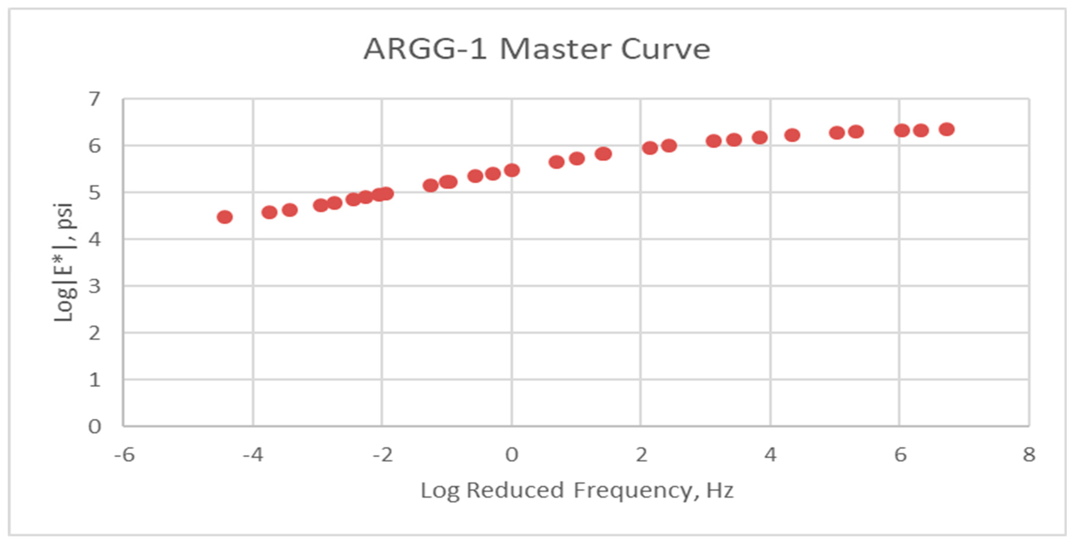
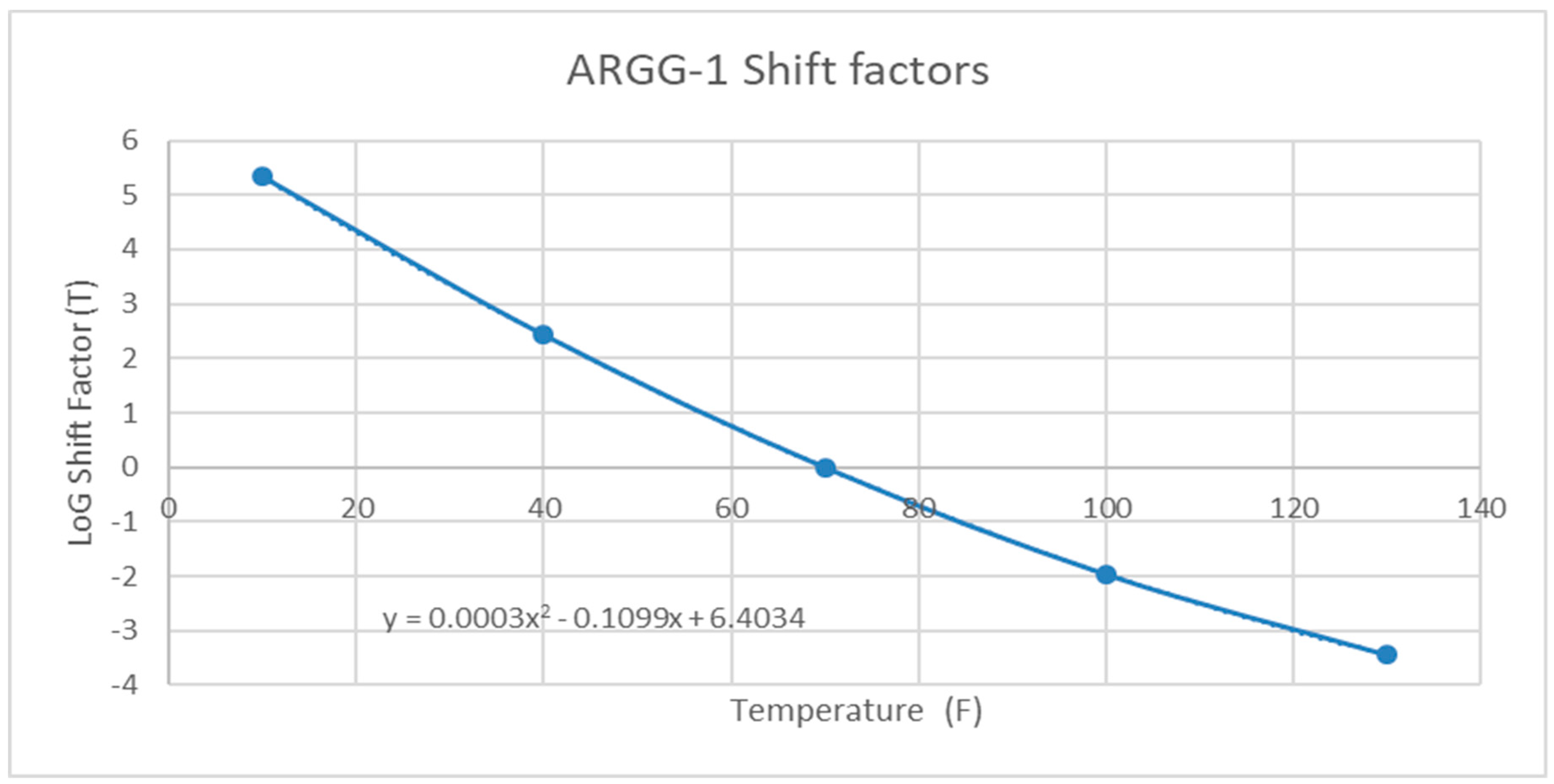
Appendix A.4.2. Dynamic Modulus (E*) Pavement ME Input
| ARGG-1 | ||||
|---|---|---|---|---|
| Temp (F) | Frequency (Hz) | |||
| 0.1 | 1 | 10 | 25 | |
| 10 | 1,688,550.19 | 1,966,960.96 | 2,175,448.5 | 2,240,515.8 |
| 40 | 687,552.7197 | 979,985.536 | 1,331,318.2 | 1,476,540 |
| 70 | 169,907.9615 | 304,180.895 | 522,202.28 | 636,736.3 |
| 100 | 56,526.39519 | 96,813.0315 | 179,173.21 | 231,341.41 |
| 130 | 29,662.06475 | 43,677.4749 | 71,655.429 | 89,572.235 |


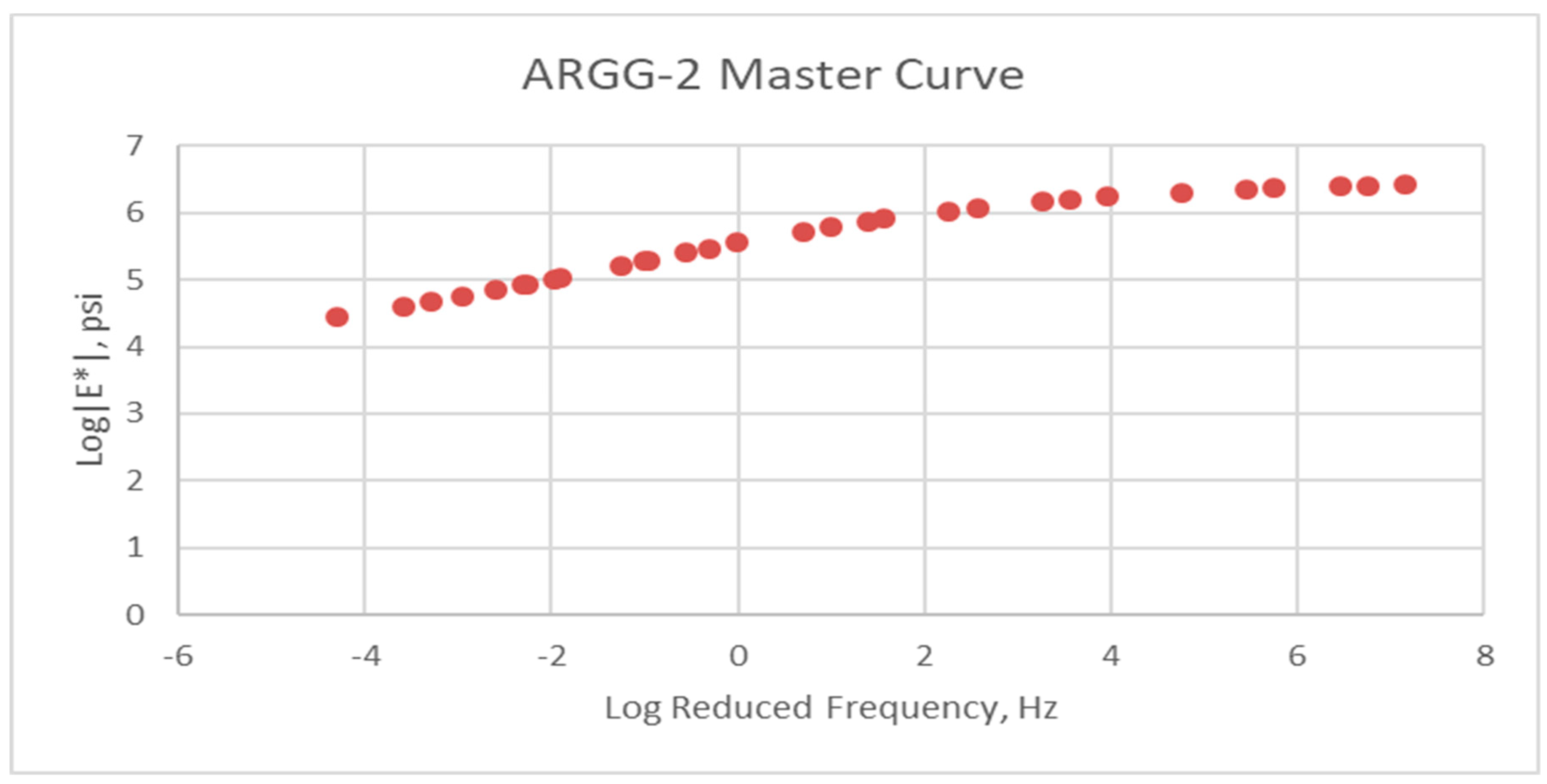
| ARGG-2 | ||||
|---|---|---|---|---|
| Temp (F) | Frequency (Hz) | |||
| 0.1 | 1 | 10 | 25 | |
| 10 | 2,014,657.96 | 2,300,848 | 2,516,240 | 2,584,199 |
| 40 | 804,896.3419 | 1,132,508 | 1,517,460 | 1,673,494 |
| 70 | 191,077.648 | 350,222.3 | 596,736.8 | 723,122.5 |
| 100 | 58,660.58927 | 106,064 | 203,032.5 | 261,578.6 |
| 130 | 28,301.08178 | 46,310.03 | 83,084.46 | 106,713.7 |

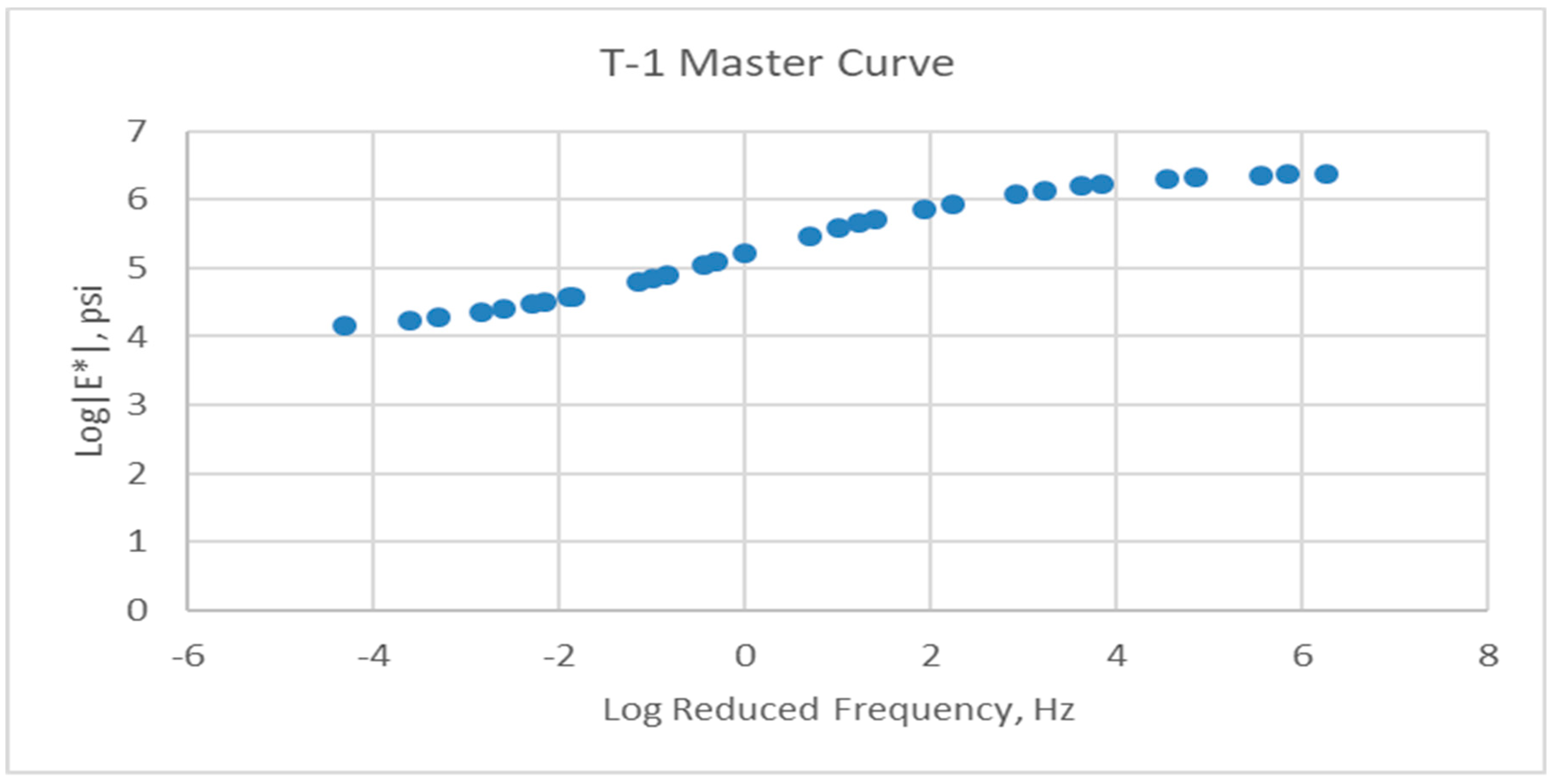
| T-1 | ||||
|---|---|---|---|---|
| Temp (F) | Frequency (Hz) | |||
| 0.1 | 1 | 10 | 25 | |
| 10 | 1,671,717.47 | 2,057,179 | 2,315,221 | 2,387,669 |
| 40 | 655,208.6218 | 1,081,775 | 1,568,820 | 1,770,225 |
| 70 | 111,555.0371 | 262,359.1 | 558,316.2 | 716,218.8 |
| 100 | 32,156.70826 | 57,201.74 | 131,883.5 | 188,498.1 |
| 130 | 14,663.03545 | 19,164.5 | 29,545.46 | 37,104.88 |


| THS-1 | ||||
|---|---|---|---|---|
| Temp (F) | Frequency (Hz) | |||
| 0.1 | 1 | 10 | 25 | |
| 10 | 2,468,122.901 | 2,773,966 | 2,962,146 | 3,013,166 |
| 40 | 1,060,744.307 | 1,530,931 | 2,067,423 | 2,278,389 |
| 70 | 198,413.424 | 427,556.5 | 820,621.8 | 1,016,861 |
| 100 | 55,629.35472 | 102,580.4 | 233,180.4 | 324,235.4 |
| 130 | 27,789.83053 | 41,829.18 | 75,808.53 | 100,861 |


| SHM-1 | ||||
|---|---|---|---|---|
| Temp (F) | Frequency (Hz) | |||
| 0.1 | 1 | 10 | 25 | |
| 10 | 1,334,184.018 | 1,721,320 | 1,987,313 | 2,061,850 |
| 40 | 323,538.2494 | 648,593.7 | 1,092,120 | 1,273,953 |
| 70 | 70,265.07206 | 135,411.7 | 289,778.7 | 390,499.8 |
| 100 | 34,666.43581 | 48,370.83 | 81,156.58 | 105,082.9 |
| 130 | 27,227.06839 | 31,853 | 41,968.07 | 48,997.99 |

| B-1 | ||||
|---|---|---|---|---|
| Temp (F) | Frequency (Hz) | |||
| 0.1 | 1 | 10 | 25 | |
| 10 | 2,389,826 | 2,739,077 | 2,977,744 | 3,047,586 |
| 40 | 1,022,230 | 1,482,512 | 1,986,847 | 2,187,285 |
| 70 | 222,885.2 | 461,931.6 | 853,728.2 | 1,047,307 |
| 100 | 53,774.47 | 112,214.4 | 255,679 | 350,569.3 |
| 130 | 21,303.35 | 37,603.73 | 77,110.14 | 105,669.7 |


| BB-1 | ||||
|---|---|---|---|---|
| Temp (F) | Frequency (Hz) | |||
| 0.1 | 1 | 10 | 25 | |
| 10 | 2,442,356.456 | 2,576,548 | 2,662,972 | 2,687,742 |
| 40 | 948,857.5471 | 1,360,029 | 1,820,795 | 2,000,413 |
| 70 | 159,373.9746 | 363,308.6 | 678,359 | 835,859.2 |
| 100 | 41,299.4409 | 81,029.95 | 185,399.2 | 256,839.6 |
| 130 | 23,343.24016 | 46,724.3 | 102,701.4 | 141,528.8 |
Appendix A.4.3. Complex Shear Modulus (G*) Pavement ME Binder Input
| B-1 | Temp (C) | Temp (F) | G* (Pa) | Phase Angle |
| PG 64-28 | 64 | 147.2 | 1193 | 86 |
| 70 | 158 | 300 | 87.5 | |
| 76 | 168.8 | 250 | 89 | |
| BB-1 | Temp (C) | Temp (F) | G* (Pa) | Phase Angle |
| PG 64-28 | 64 | 147.2 | 1107 | 82.93 |
| 70 | 158 | 300 | 85.97 | |
| 76 | 168.8 | 250 | 89 | |
| ARGG-1 | Temp (C) | Temp (F) | G* (Pa) | Phase Angle |
| PG 58-28 | 58 | 136.4 | 1505 | 85.93 |
| 64 | 147.2 | 700 | 87.47 | |
| 70 | 158 | 300 | 89 | |
| ARGG-2 | Temp (C) | Temp (F) | G* (Pa) | Phase Angle |
| PG 58-28 | 58 | 136.4 | 1479 | 86.18 |
| 64 | 147.2 | 700 | 87.59 | |
| 70 | 158 | 300 | 89 | |
| T-1 | Temp (C) | Temp (F) | G* (Pa) | Phase Angle |
| PG 64-28 | 64 | 147.2 | 1100 | 82.76 |
| 70 | 158 | 300 | 85.88 | |
| 76 | 168.8 | 250 | 89 | |
| THS-1 | Temp (C) | Temp (F) | G* (Pa) | Phase Angle |
| PG 76-28 | 76 | 168.8 | 1301 | 67.83 |
| 82 | 179.6 | 200 | 78.42 | |
| 88 | 190.4 | 100 | 89 | |
| SHM-1 | Temp (C) | Temp (F) | G* (Pa) | Phase Angle |
| PG 70-34 | 70 | 158 | 1245 | 54.21 |
| 76 | 168.8 | 250 | 71.61 | |
| 82 | 179.6 | 200 | 89 |
Appendix A.5. Maintenance and Rehabilitation Alternative Emission Results
| ARGG-1 Cross Section | |||
|---|---|---|---|
| Baseline | Energy [MJ] | CO2 [Mg] = GWP | |
| Initial Construction | Materials Production | 37,972,888,683 | 2,004,224 |
| Materials Transportation | 2,003,300,632 | 149,765 | |
| Processes (Equipment) | 193,655,431 | 14,535 | |
| SUM | 40,169,844,745 | 2,168,524 | |
| Mill and Fill | Energy [MJ] | CO2 [Mg] = GWP | |
| Maintenance | Materials Production | 6,865,339,512 | 368,288 |
| Materials Transportation | 405,995,727 | 30,352 | |
| Processes (Equipment) | 54,425,489 | 4,085 | |
| SUM | 7,325,760,728 | 402,725 | |
| CIR | Energy [MJ] | CO2 [Mg] = GWP | |
| Maintenance | Materials Production | 5,149,004,634 | 276,216 |
| Materials Transportation | 340,644,743 | 25,466 | |
| Processes (Equipment) | 49,098,146 | 3,685 | |
| SUM | 5,538,747,523 | 305,368 | |
| Microsurface | Energy [MJ] | CO2 [Mg] = GWP | |
| Maintenance | Materials Production | 3,432,669,756 | 184,144 |
| Materials Transportation | 275,293,760 | 20,581 | |
| Processes (Equipment) | 41,779,821 | 3,136 | |
| SUM | 3,749,743,337 | 207,861 | |
| ARGG-2 Cross Section | |||
|---|---|---|---|
| Baseline | Energy [MJ] | CO2 [Mg] = GWP | |
| Initial Construction | Materials Production | 37,972,888,683 | 2,004,224 |
| Materials Transportation | 2,003,300,632 | 149,765 | |
| Processes (Equipment) | 193,655,431 | 14,535 | |
| SUM | 40,169,844,745 | 2,168,524 | |
| Mill and Fill | Energy [MJ] | CO2 [Mg] = GWP | |
| Maintenance | Materials Production | 6,795,577,992 | 363,862 |
| Materials Transportation | 412,709,701 | 30,854 | |
| Processes (Equipment) | 55,053,496 | 4,132 | |
| SUM | 7,263,341,189 | 398,848 | |
| CIR | Energy [MJ] | CO2 [Mg] = GWP | |
| Maintenance | Materials Production | 5,096,683,494 | 272,897 |
| Materials Transportation | 345,680,224 | 25,843 | |
| Processes (Equipment) | 49,569,152 | 3,720 | |
| SUM | 5,491,932,870 | 302,460 | |
| Microsurface | Energy [MJ] | CO2 [Mg] = GWP | |
| Maintenance | Materials Production | 3,397,788,996 | 181,931 |
| Materials Transportation | 278,650,747 | 20,832 | |
| Processes (Equipment) | 42,093,825 | 3,159 | |
| SUM | 3,718,533,568 | 205,922 | |
| THS-1 Cross Section | |||
|---|---|---|---|
| Baseline | Energy [MJ] | CO2 [Mg] = GWP | |
| Initial Construction | Materials Production | 37,972,888,683 | 2,004,224 |
| Materials Transportation | 2,003,300,632 | 149,765 | |
| Processes (Equipment) | 193,655,431 | 14,535 | |
| SUM | 40,169,844,745 | 2,168,524 | |
| Mill and Fill | Energy [MJ] | CO2 [Mg] = GWP | |
| Maintenance | Materials Production | 5,381,887,465 | 284,662 |
| Materials Transportation | 404,968,158 | 30,275 | |
| Processes (Equipment) | 54,198,337 | 4,068 | |
| SUM | 5,841,053,960 | 319,005 | |
| CIR | Energy [MJ] | CO2 [Mg] = GWP | |
| Maintenance | Materials Production | 4,036,415,599 | 213,497 |
| Materials Transportation | 339,874,066 | 25,409 | |
| Processes (Equipment) | 48,927,782 | 3,672 | |
| SUM | 4,425,217,448 | 242,578 | |
| Microsurface | Energy [MJ] | CO2 [Mg] = GWP | |
| Maintenance | Materials Production | 2,690,943,733 | 142,331 |
| Materials Transportation | 274,779,975 | 20,542 | |
| Processes (Equipment) | 41,666,245 | 3,127 | |
| SUM | 3,007,389,953 | 166,001 | |
| T-1 Cross Section | |||
|---|---|---|---|
| Baseline | Energy [MJ] | CO2 [Mg] = GWP | |
| Initial Construction | Materials Production | 37,972,888,683 | 2,004,224 |
| Materials Transportation | 2,003,300,632 | 149,765 | |
| Processes (Equipment) | 193,655,431 | 14,535 | |
| SUM | 40,169,844,745 | 2,168,524 | |
| Mill and Fill | Energy [MJ] | CO2 [Mg] = GWP | |
| Maintenance | Materials Production | 5,442,180,423 | 287,509 |
| Materials Transportation | 412,579,971 | 30,844 | |
| Processes (Equipment) | 54,922,550 | 4,122 | |
| SUM | 5,909,682,943 | 322,475 | |
| CIR | Energy [MJ] | CO2 [Mg] = GWP | |
| Maintenance | Materials Production | 4,081,635,317 | 215,631 |
| Materials Transportation | 345,582,926 | 25,835 | |
| Processes (Equipment) | 49,470,942 | 3,713 | |
| SUM | 4,476,689,185 | 245,180 | |
| Microsurface | Energy [MJ] | CO2 [Mg] = GWP | |
| Maintenance | Materials Production | 2,721,090,211 | 143,754 |
| Materials Transportation | 278,585,882 | 20,827 | |
| Processes (Equipment) | 42,028,352 | 3,154 | |
| SUM | 3,041,704,445 | 167,736 | |
| SHM-1 Cross Section | |||
|---|---|---|---|
| Baseline | Energy [MJ] | CO2 [Mg] = GWP | |
| Initial Construction | Materials Production | 37,972,888,683 | 2,004,224 |
| Materials Transportation | 2,003,300,632 | 149,765 | |
| Processes (Equipment) | 193,655,431 | 14,535 | |
| SUM | 40,169,844,745 | 2,168,524 | |
| Mill and Fill | Energy [MJ] | CO2 [Mg] = GWP | |
| Maintenance | Materials Production | 5,492,078,801 | 290,431 |
| Materials Transportation | 411,118,915 | 30,735 | |
| Processes (Equipment) | 54,788,931 | 4,112 | |
| SUM | 5,957,986,647 | 325,278 | |
| CIR | Energy [MJ] | CO2 [Mg] = GWP | |
| Maintenance | Materials Production | 4,119,059,101 | 217,823 |
| Materials Transportation | 344,487,134 | 25,754 | |
| Processes (Equipment) | 49,370,728 | 3,706 | |
| SUM | 4,512,916,963 | 247,282 | |
| Microsurface | Energy [MJ] | CO2 [Mg] = GWP | |
| Maintenance | Materials Production | 2,746,039,401 | 145,215 |
| Materials Transportation | 277,855,354 | 20,772 | |
| Processes (Equipment) | 41,961,542 | 3,149 | |
| SUM | 3,065,856,297 | 169,137 | |
References
- American Society of Civil Engineers (ASCE). 2017 Infrastructure Report Card—Roads. 2017. Available online: http://www.infrastructurereportcard.org/wp-content/uploads/2017/01/Roads-Final.pdf (accessed on 6 November 2018).
- TRIP. National Fact Sheet. September 2018. Available online: http://www.tripnet.org/docs/Fact_Sheet_National.pdf (accessed on 6 May 2018).
- Wang, T.; Lee, I.S.; Kendall, A.; Harvey, J.; Lee, E.B.; Kim, C. Life cycle energy consumption and GHG emission from pavement rehabilitation with different rolling resistance. J. Clean. Prod. 2012, 33, 86–96. [Google Scholar] [CrossRef]
- Kang, S.; Yang, R.; Ozer, H.; Al-Qadi, I.L. Life-cycle greenhouse gases and energy consumption for material and construction phases of pavement with traffic delay. Transp. Res. Rec. 2014, 2428, 27–34. [Google Scholar] [CrossRef]
- Qing, L.; Fred, L.M.; Xin, C. A Life Cycle Assessment Framework for Pavement Maintenance and Rehabilitation Technologies or An Integrated Life Cycle Assessment (LCA)–Life Cycle Cost Analysis (LCCA) Framework for Pavement Maintenance and Rehabilitation; Center for Transportation, Environment, and Community Health (CTECH) Final Report. US DOT; 31 January 2018. [Google Scholar]
- Pavement Life Cycle Assessment Workshop. University of California: Davis, CA, USA, May 2010. Available online: http://www.ucprc.ucdavis.edu/p-lca/presentations.html (accessed on 6 November 2018).
- Ventura, A.; Roche, C.D.L. International Symposium on Life Cycle Assessment and Construction—Civil Engineering and Buildings; 2012 RILEM Publications SARL; ISBN 978-2-35158-127-8.
- International Symposium on Pavement LCA 2014. Pavement LCA 2014. 2014. Available online: http://www.ucprc.ucdavis.edu/p-lca2014/Papers.aspx (accessed on 14 March 2019).
- Al-Qadi, I.; Ozer, H.; Harvey, J. Pavement LCA Symposium 2017. University of Illinois at Urbana-Champaign: Champaign, April 2017. Available online: http://lcasymposium.ict.illinois.edu/proceedings/ (accessed on 14 March 2019).
- Harvey, J.; Meijer, J.; Al-Qadi, I.L.; Saboori, A. Pavement Life Cycle Assessment Framework; Federal Highway Administration: Washington, DC, USA, July 2016. Available online: http://www.fhwa.dot.gov/pavement/sustainability/hif16014.pdf (accessed on 28 January 2019).
- Zaabar, I.; Karim, C. Calibration of HDM-4 models for estimating the effect of pavement roughness on fuel consumption for US conditions. Transp. Res. Rec. J. Transp. Res. Board 2010, 2155, 105–116. [Google Scholar] [CrossRef]
- Chatti, K.; Imen, Z. Estimating the Effects of Pavement Condition on Vehicle Operating Costs; Transportation Research Board: Washington, DC, USA, 2012; Volume 720. [Google Scholar]
- Robbins, M.M.; Tran, N. Literature review: The effect of pavement roughness on vehicle operating costs. Natl. Cent. Asph. Technol. Rep. 2015. Available online: http://www.eng.auburn.edu/research/centers/ncat/files/technical-reports/rep15-02.pdf (accessed on 28 January 2019).
- Ziyadi, M.; Ozer, H.; Kang, S.; Al-Qadi, I.L. Vehicle energy consumption and an environmental impact calculation model for the transportation infrastructure systems. J. Clean. Prod. 2018, 174, 424–436. [Google Scholar] [CrossRef]
- DeCarlo, C.; Mo, W.; Dave, E.V.; Locore, J. Sustainable Pavement Rehabilitation Strategy Using Consequential Life Cycle Assessment. In Proceedings of the 10th International Conference on the Bearing Capacity of Roads, Railways and Airfields, Athens, Greece, 28–30 June 2017. [Google Scholar] [CrossRef]
- MassDOT. Transportation Data Management System (MS2). 2018. Available online: http://mhd.ms2soft.com/tcds/tsearch.asp?loc=Mhd&mod= (accessed on 9 April 2018).
- Google. Google maps. Available online: https://www.google.com/maps/dir/42.603823,-71.3501962/42.7392095,-71.1416834/@42.7452328,-71.134279,14.71z/data=!4m2!4m1!3e0 (accessed on 8 January 2018).
- Nemati, R.; Dave, E.V.; Daniel, J.S. Statistical Evaluation of Effect of Mix Design Properties on Performance Indices of Asphalt Mixtures. ASTM J. Test. Eval. 2019, in press. [Google Scholar]
- SimaPro 8.0.0 (2013). Software. Available online: https://simapro.com (accessed on 12 June 2019).
- Horvath, A. Pavement Life-Cycle Assessment Tool for Environmental and Economic Effects (PaLATE); Consortium on Green Design and Manufacturing from the University of California-Berkeley; University of California-Berkeley: Berkeley, CA, USA, 2013. [Google Scholar]
- CalTrans. LIFE-CYCLE COST ANALYSIS PROCEDURES MANUAL; California Department of Transportation: Sacramento, CA, USA, 2013; p. 158. [Google Scholar]
- Mousa, M.; Elseifi, M.A.; Bashar, M.; Zhang, Z.; Gaspard, K. Field Evaluation and Cost Effectiveness of Crack Sealing in Flexible and Composite Pavements. Transp. Res. Rec. J. Transp. Res. Board 2018, 2672, 51–61. [Google Scholar] [CrossRef]
- Cole, M.; Geib, J. MnDOT’s Experience: Efforts to Improve Micro Surfacing Performance. 2016. Available online: https://www.dot.state.mn.us/materials/pavementpreservation/mndotexperiences/documents/EffortstoImproveMicroSurfacingPerformance.pdf (accessed on 9 April 2018).
- Damp, S. Cold In-Place Recycling: Southeast Pavement Preservation Partnership. Available online: http://www.pavementpreservation.org/wp-content/uploads/presentations/Cold%20In-Place%20Recycling.pdf (accessed on 9 April 2018).
- Lane, B.; Kazmierowski, T. Short Term Performance of an Innovative Cold In-Place Recycling Technology in Ontario. In Proceedings of the 2005 Annual Conference of the Transportation Association of Canada, Calgary, AB, Canada, 18–21 September 2005; Available online: http://conf.tac-atc.ca/english/resourcecentre/readingroom/conference/conf2005/docs/s15/lane.pdf (accessed on 9 April 2018).
- Fitts, G.L. Thin Overlays for Pavement Preservation and Functional Rehabilitation. Available online: http://www.ltrc.lsu.edu/ltc_09/pdf/Fitts,%20Gary.pdf (accessed on 6 May 2018).
- Nair, H.; McGhee, K.K.; Habib, A.; Shatty, S. Assessment of an Incentive Only Ride Specification for Asphalt Pavements; Final Report VCTIR 16-R2; Virginia Center for Transportation Innovation and Research: Charlottesville, VA, USA, 10 September 2015. [Google Scholar]
- Transportation Research Board (TRB). InSight Data Access Website—SHRP2 Naturalistic Driving Study. 2018. Available online: https://insight.shrp2nds.us/ (accessed on 9 April 2018).
- Environmental Protection Agency (EPA). MOtor Vehicles Emissions Simulator (MOVES), MOVES2014a ed.; EPA: Washington, DC, USA, 2014. [Google Scholar]
- AASHTOWare. Pavement ME Design; Version 2.3; AASHTOWare: Washington, DC, USA, 17 July 2015. [Google Scholar]
- Wilde, J.W. Implementation of An International Roughness Index for mn/DOT Pavement Construction and Rehabilitation; No. MN/RC-2007-09; Minnesota Department of Transportation: Saint Paul, MN, USA, 2007; Available online: http://www.lrrb.org/PDF/200709.pdf (accessed on 9 January 2019).
- Loprencipe, G.; Pantuso, A.; Di Mascio, P. Sustainable pavement management system in urban areas considering the vehicle operating costs. Sustainability 2017, 9, 453. [Google Scholar] [CrossRef]
- Kerali, H.G. HDM-4: Highway Development and Management: Volume One: Overview of HDM-4; The World Road Association (PIARC): Paris, France; The World Bank: Washington, DC, USA, 2000. [Google Scholar]
- Walls, J.; Smith, M.R. Life-Cycle Cost Analysis in Pavement Design: In Search of Better Investment Decisions; Federal Highway Administration: Washington, DC, USA, 1998.
- New England (PADD 1A) Regular All Formulations Retail Gasoline Prices. Petroleum and Other Liquids. US Energy Information Administration, April 2017. Available online: http://www.eia.gov/petroleum/gasdiesel/ (accessed on 6 May 2018).
- Ogwang, A.; Samer, M.; Arpad, H. Optimal Cracking Threshold Resurfacing Policies in Asphalt Pavement Management to Minimize Costs and Emissions. J. Infrastruct. Syst. 2019, 25. [Google Scholar] [CrossRef]
- Pantuso, A.; Loprencipe, G.; Bonin, G.; Teltayev, B.B. Analysis of pavement condition survey data for effective implementation of a network level pavement management program for Kazakhstan. Sustainability 2019, 11, 901. [Google Scholar] [CrossRef]
- Chehovits, J.; Larry, G. Energy usage and greenhouse gas emissions of pavement preservation processes for asphalt concrete pavements. In Proceedings of the 1st International Conference of Pavement Preservation, Newport Beach, CA, USA, 13–15 April 2010. [Google Scholar]


| Mixture Name | Course Description | Layer Thickness (cm) | Asphalt Binder Type | Amount of Recycled Asphalt Pavement in the Mix (% by Total Weight of Mix) |
|---|---|---|---|---|
| ARGG-1 | Surface | 5 | PG 58-28 | 10 |
| ARGG-2 | Surface | 5 | PG 58-28 | 0 |
| T-1 | Surface | 5 | PG 64-28 | 19.3 |
| THS-1 | Surface | 5 | PG 76-28 | 19.3 |
| SHM-1 | Surface | 5 | PG 70-34 | 0 |
| B-1 | Binder | 20 | PG 64-28 | 25 |
| BB-1 | Base | 20 | PG 64-28 | 25 |
| GB | Granular Base | 60 | - | - |
| Scenario | Gasoline Price ($) | Diesel Price ($) |
|---|---|---|
| Low | 1.64 | 1.71 |
| Current | 2.80 | 3.00 |
| High | 4.04 | 4.66 |
| Maintenance Alternative | ||||||||||||
|---|---|---|---|---|---|---|---|---|---|---|---|---|
| Cross-Section | DNR | CIR | CS | MO | MS 2.2 m/km | MS 2.5 m/km | ||||||
| C/M | O | C/M | O | C/M | O | C/M | O | C/M | O | C/M | O | |
| Gg CO2 eq | ||||||||||||
| ARGG-1 | 78 | 436 | 29 | 436 | 15 | 430 | 30 | 437 | 53 | 434 | 44 | 437 |
| ARGG-2 | 77 | 435 | 26 | 435 | 72 | 436 | 29 | 435 | 52 | 435 | 55 | 438 |
| SHM-1 | 73 | 430 | 27 | 436 | 52 | 435 | - | - | 54 | 436 | 26 | 437 |
| T-1 | 119 | 434 | 43 | 435 | 107 | 434 | 78 | 436 | 101 | 436 | 75 | 435 |
| THS-1 | 83 | 435 | 34 | 437 | 91 | 435 | - | - | 75 | 436 | 61 | 435 |
| Maintenance Alternative | ||||||||||||
|---|---|---|---|---|---|---|---|---|---|---|---|---|
| Cross-Section | DNR | CIR | CS | MO | MS 2.2 m/km | MS 2.5 m/km | ||||||
| C/M | O | C/M | O | C/M | O | C/M | O | C/M | O | C/M | O | |
| Millions of Dollars | ||||||||||||
| ARGG-1 | 232 | 3213 | 158 | 3214 | 219 | 3231 | 157 | 3215 | 187 | 3209 | 191 | 3232 |
| ARGG-2 | 231 | 3213 | 158 | 3215 | 219 | 3219 | 157 | 3216 | 187 | 3210 | 156 | 3224 |
| SHM-1 | 299 | 3145 | 160 | 3147 | 277 | 3146 | - | - | 253 | 3144 | 215 | 3145 |
| T-1 | 232 | 3213 | 158 | 3177 | 224 | 3179 | 157 | 3178 | 187 | 3171 | 191 | 3186 |
| THS-1 | 267 | 3209 | 159 | 3203 | 252 | 3196 | - | - | 219 | 3200 | 199 | 3193 |
© 2019 by the authors. Licensee MDPI, Basel, Switzerland. This article is an open access article distributed under the terms and conditions of the Creative Commons Attribution (CC BY) license (http://creativecommons.org/licenses/by/4.0/).
Share and Cite
Haslett, K.E.; Dave, E.V.; Mo, W. Realistic Traffic Condition Informed Life Cycle Assessment: Interstate 495 Maintenance and Rehabilitation Case Study. Sustainability 2019, 11, 3245. https://doi.org/10.3390/su11123245
Haslett KE, Dave EV, Mo W. Realistic Traffic Condition Informed Life Cycle Assessment: Interstate 495 Maintenance and Rehabilitation Case Study. Sustainability. 2019; 11(12):3245. https://doi.org/10.3390/su11123245
Chicago/Turabian StyleHaslett, Katie E., Eshan V. Dave, and Weiwei Mo. 2019. "Realistic Traffic Condition Informed Life Cycle Assessment: Interstate 495 Maintenance and Rehabilitation Case Study" Sustainability 11, no. 12: 3245. https://doi.org/10.3390/su11123245
APA StyleHaslett, K. E., Dave, E. V., & Mo, W. (2019). Realistic Traffic Condition Informed Life Cycle Assessment: Interstate 495 Maintenance and Rehabilitation Case Study. Sustainability, 11(12), 3245. https://doi.org/10.3390/su11123245