Asphalt Pavement Acoustic Performance Model


Abstract
:1. Introduction
- Identifing field test sections with a low noise of road surfaces for field noise evaluation and asphalt mixture composition evaluation.
- Collecting field core samples of the various pavement types.
- Assembling and documenting the mixture’s material properties and field noise measurements.
- Analyzing correlations between the asphalt mixture’s composition and volumetric properties and noise level.
- Observing the asphalt pavement’s acoustical performance (noise) prediction models using mathematical relationships, which are fundamentally based on the road mixture’s volumetric properties.
- Evaluating the sensitivity of the established noise-level prediction model.
2. Background of Pavement Acoustical Performance
3. Materials and Methods
3.1. Low-Noise Pavement Sections
3.2. Tests Methods
3.3. Analysis Methods
- Linear relationship. The relationships between Yi and each of the independent variables Xi, are linear. This assumption was tested by calculating the Pearson coefficient of correlation.
- No or little multicollinearity. Multicollinearity occurs when the independent variables are not independent of each other. This assumption was tested using variance inflation factor (VIF) values. A variance inflation factor quantifies how much the variance is inflated. The standard errors and the variances of the estimated coefficients are inflated when a multicollinearity exists. The variance inflation factor VIFi for the estimated coefficient Âi is calculated using the formula:where is the R2—the value obtained by Xi and each of the independent variables. If VIFi > 4, the variable Xi causes the problem of multicollinearity in the model [33].
- Multivariate normality. Multiple regression assumes that the residuals are normally distributed. This assumption is tested using the Shapiro–Wilk test. If the test statistic has a p-value < 0.05, then the null hypothesis that residuals are normally distributed is rejected.
- Homoscedasticity. This assumption states that the variance of error terms is similar across the values of the independent variables. This assumption was tested using the Breusch–Pagan test. Before deciding upon an estimation method, one may conduct the Breusch–Pagan test to examine the presence of heteroscedasticity. The Breusch–Pagan test assumes that the error terms are normally distributed. If the test statistic has a p-value < 0.05, then the null hypothesis of homoscedasticity is rejected, and heteroscedasticity is assumed [34].
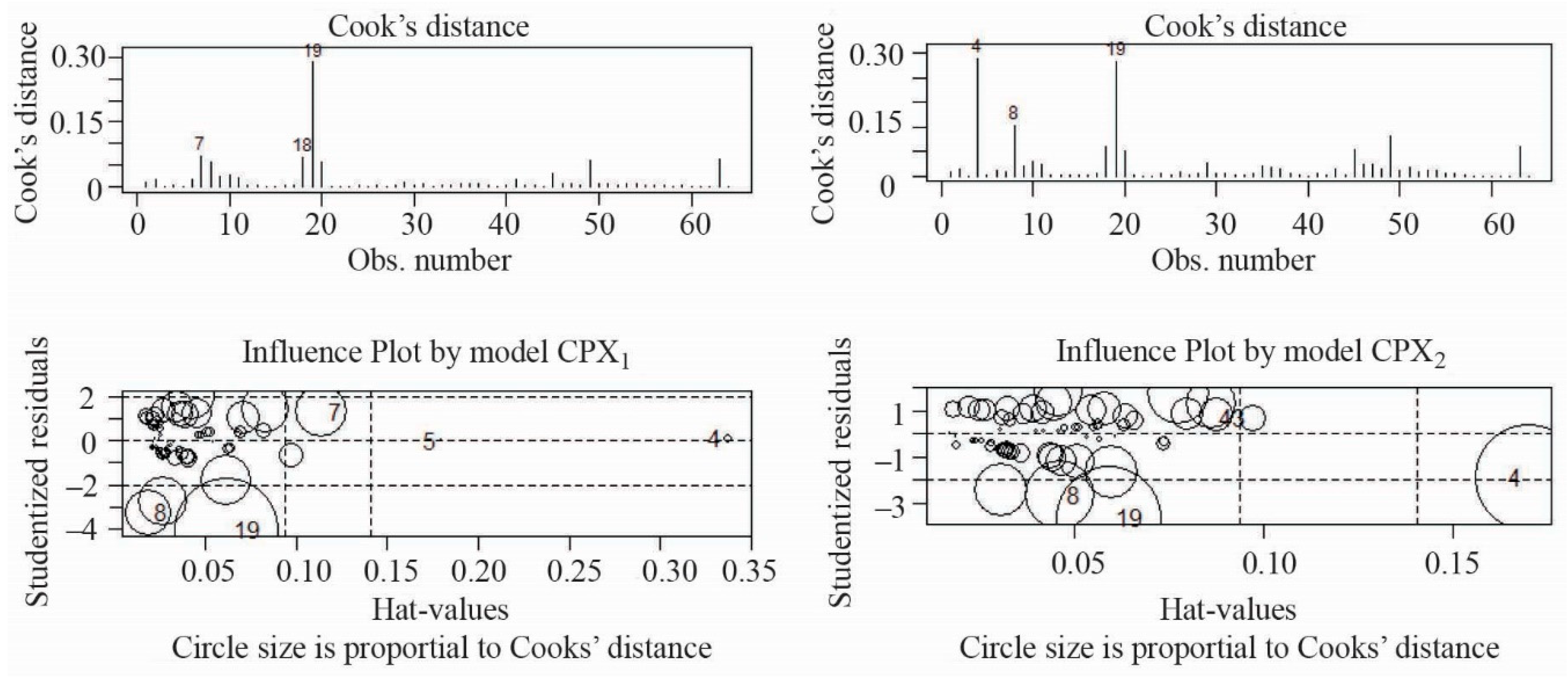
- Outliers. We assume that all special causes, outliers due to one-time situations, have been removed from the data. If not, they may cause a non-constant variance, non-normality, or other problems with the regression model. This assumption was tested using the Bonferroni test. If the test statistic has a p-value < 0.05, then it is assumed that the data contain outliers [35].
4. Results and Analysis
4.1. Properties of Low-Noise Asphalt Mixtures
4.2. Properties of Low-Noise Asphalt Mixtures
4.3. Pavement Acoustic Properties Prediction Model
5. Conclusions
- The composition of the asphalt mixture in the investigated test sections significantly varies depending on the manufacturer:
- The bitumen content varies from 5.4% to 5.84% for AC 11 VN, from 4.38% to 4.88% for SA 16, from 5.87% to 6.65% for SMA 11 S, from 5.91% to 6.9% for SMA 8 TM and from 6.80% to 7.20% for SMA 8 S asphalt mixtures;
- The air-void content varies from 1.0% to 3.7% for AC 11 VN, from 2.7% to 7.7% for SA 16, from 1.6% to 3.9% for SMA 11 S, from 6.3% to 11.6% for SMA 8 TM and from 3.5% to 5.3% for SMA 8 S asphalt mixtures;
- Voids in mineral aggregate (VMA) values vary from 12.5% to 13.7% for AC 11 VN, from 10.1% to 11.3% for SA 16, from 13.8% to 15.4% for SMA 11 S, from 13.1% to 15.9% for SMA 8 TM and from 15.1% to 16.5% for SMA 8 S asphalt mixtures;
- Voids filled with bitumen (VFB) values vary from 78.3% to 92.8% for AC 11 VN, from 58.3% to 78.8% for SA 16, from 78.5% to 90.5% for SMA 11 S, from 54.0% to 71.7% for SMA 8 TM and from 74.2% to 82.3% for SMA 8 S asphalt mixtures.
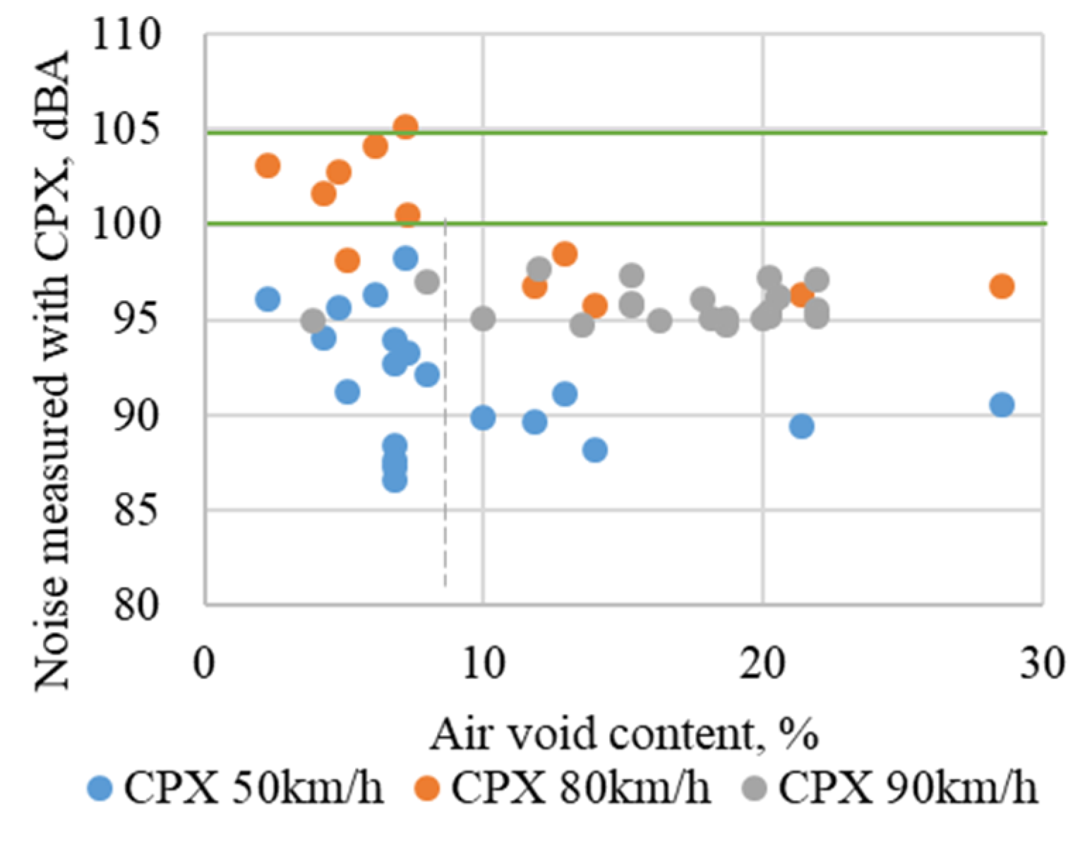
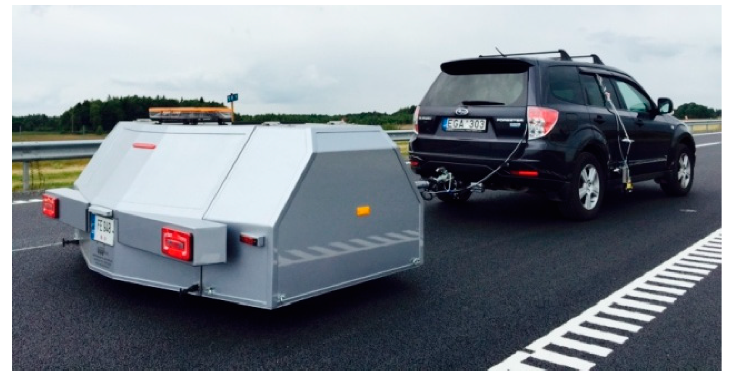
- The tire/road noise measurements were performed at 80 km/h using the CPX method for pavement sections at the first year of exploitation. The average noise level generated from tire/pavement interactions was 97.2 dB(A) with a standard deviation of 1.38; therefore, all analyzed pavements comply definition of low-noise pavements.
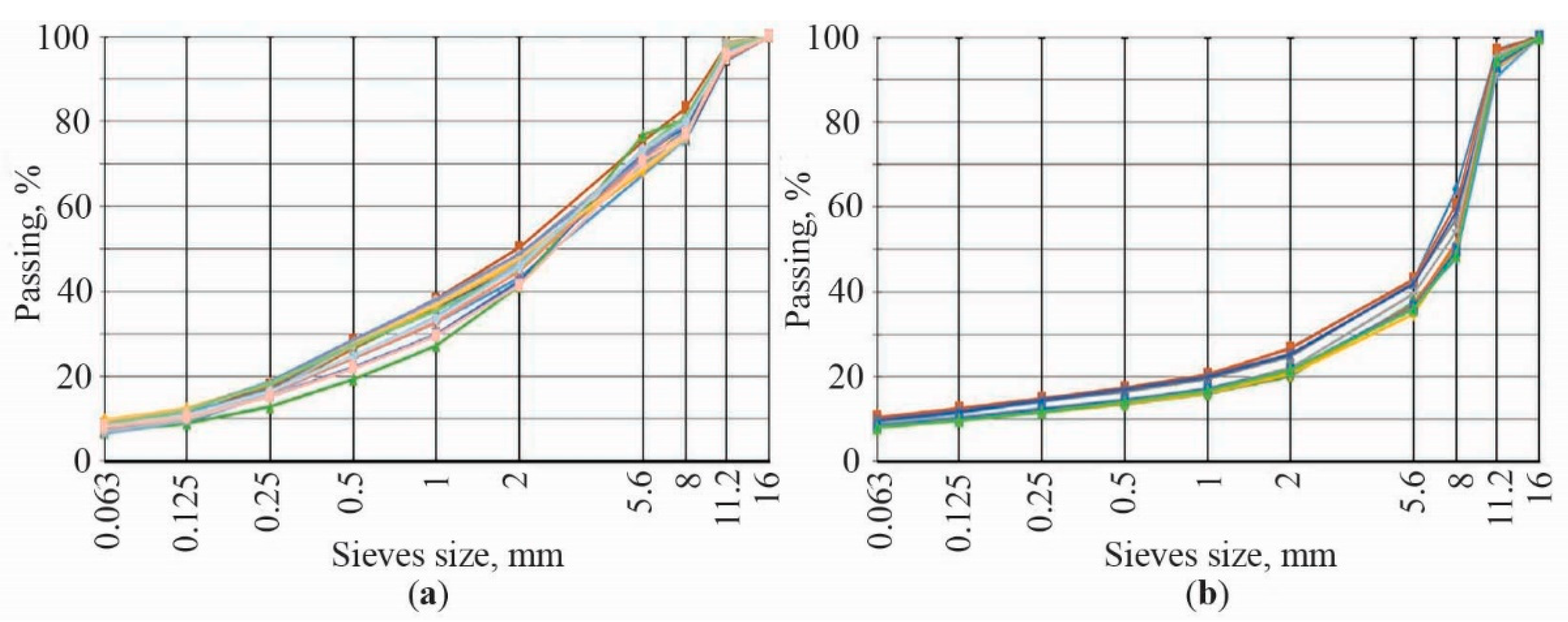
- According to the correlation analysis of the noise level and components of the low-noise asphalt mixture, it can be stated that CPX80 is highly correlated in terms of the percentage of aggregates passing through a 8.0 mm and 11.2 mm sieve size, the density of the mineral aggregate, the apparent density of the asphalt mixture, air-void content, voids in the mineral aggregate and voids in the mineral aggregate filled with bitumen.
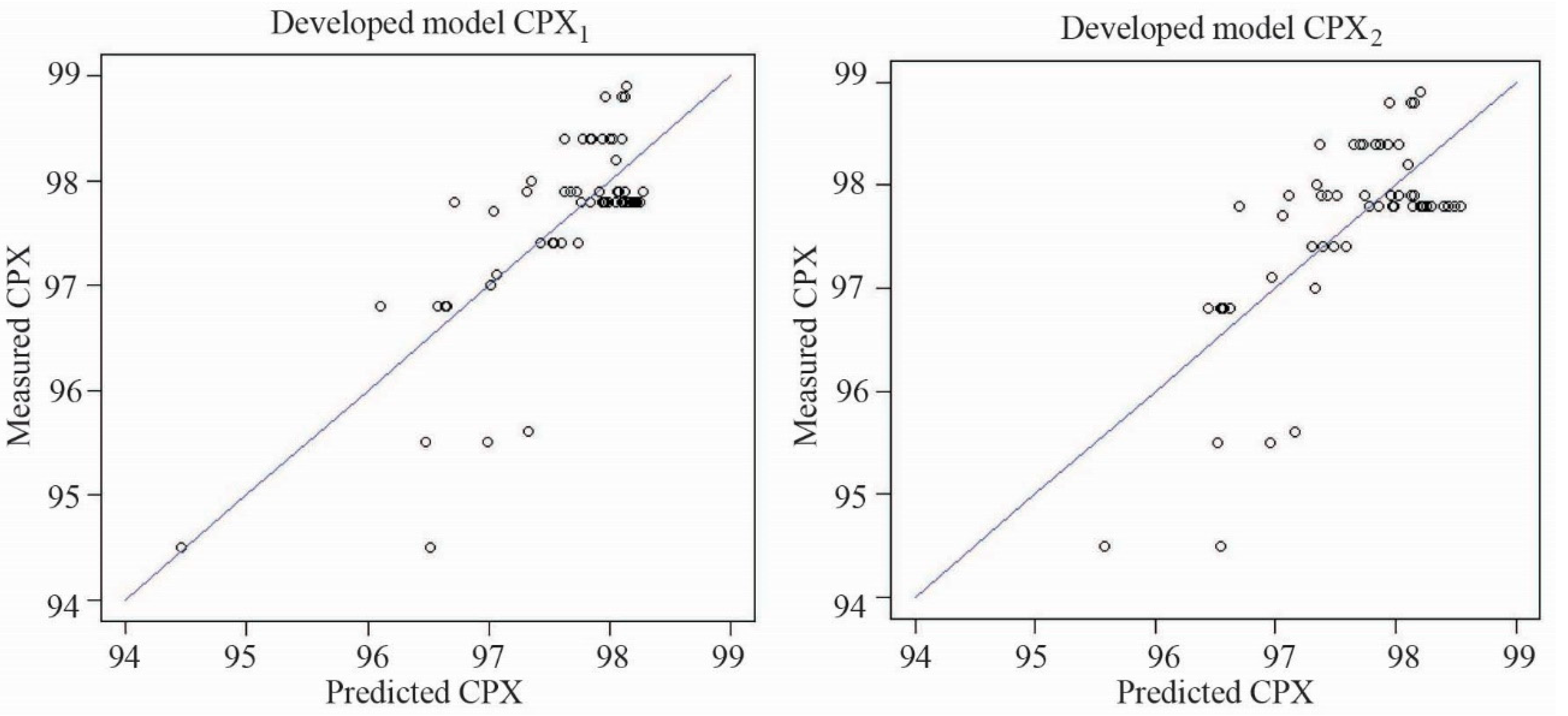
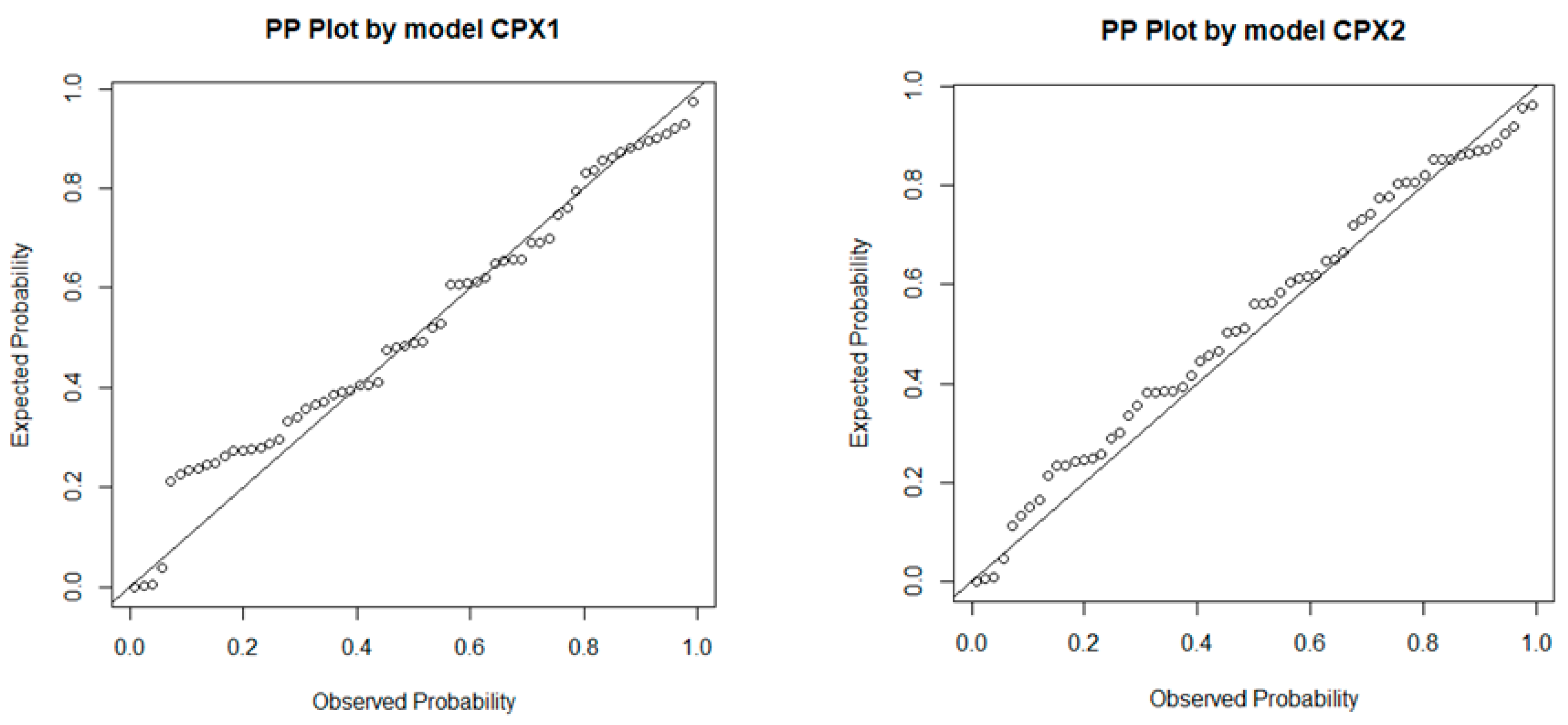
- During the analysis of the collected database on low-noise asphalt pavements, two pavement acoustic models were obtained, CPX1 and CPX2, for which the coefficients of determinations were 0.59 and 0.50, respectively. However, the normality assumption of the Shapiro–Wilk test was not satisfied, mainly due to the limited database.
- The analysis showed that there is a reasonable link between the composition of the asphalt wearing layer and the tire/road noise level. However, in order to provide a more complex prediction model, a database of low-volume asphalt mixtures should include no less than three different asphalt compositions, pavement textures and G-factor values for each type of asphalt mixture.
Author Contributions
Funding
Conflicts of Interest
Abbreviation
| AADT | annual average daily traffic |
| AC | dense asphalt concrete |
| ANOVA | basic analysis of variance |
| CPX | close-proximity method |
| DAMP | damping acoustical measurement parameter |
| ERNL | estimated road noisiness level |
| HMA | hot mix asphalt |
| Gmb | bulk specific gravity of compacted mixture |
| Gmm | maximum theoretical specific gravity |
| MPD | mean profile depth |
| NMS | nominal maximum size of asphalt mixture aggregates |
| OBSI | on-board sound intensity method |
| p0.063, p0.125 … p11.2 | aggregate gradation sieve no and mesh size, mm |
| PA | porous asphalt |
| PP | probability–probability plot |
| Pb | bitumen content |
| SA | specific surface area of the aggregate |
| SI | shape index |
| SIL or IL | sound intensity level or intensity level |
| SMA | stone mastic asphalt mixture |
| TNM | traffic noise model |
| TMOA | low noise asphalt mixture |
| VA | air-void content |
| VIF | variance inflation factor |
| VFB | voids filed with bitumen |
| VMA | voids in mineral aggregate |
References
- Regional Office Europe (WHO). Night Noise Guidelines for Europe; WHO Regional Office Europe: København, Denmark, 2014. [Google Scholar]
- EC. Report from the Commission to the European Parliament and the Council: On the Implementation of the Environmental Noise Directive in Accordance with Article 11 of Directive 2002/49/EC; COM (2011) 321 final; EC: Brussel, Belgium, 2011. [Google Scholar]
- Vaitkus, A.; Vorobjovas, V.; Jagniatinskis, A.; Andriejauskas, T.; Fiks, B. Peculiarity of low noise pavement design under Lithuanian conditions. Balt. J. Road Bridg. Eng. 2014, 9, 155–163. [Google Scholar] [CrossRef]
- Zofka, E.; Zofka, A.; Mechowski, T. Pavement noise measurements in Poland. In IOP Conference Series Materials Science and Engineering; IOP Publishing: Bristol, UK, 2017; Volume 236. [Google Scholar]
- Bernhard, R.; Wayson, R. An introduction to tire/pavement noise of asphalt pavement. Inst. Safe Quiet 2005, 26, 27. [Google Scholar]
- Donavan, P.R.; Rymer, B. Assessment of highway pavements for tire/road noise generation. SAE Trans. 2003, 112, 1829–1838. [Google Scholar]
- Vaitkus, A.; Andriejauskas, T.; Vorobjovas, V.; Jagniatinskis, A.; Fiks, B.; Zofka, E. Asphalt wearing course optimization for road traffic noise reduction. Constr. Build. Mater. 2017, 152, 345–356. [Google Scholar] [CrossRef]
- Sandberg, U.; Ejsmont, J. Tire/Road Noise Reference Book; INFORMEX: Kisa, Sweden, 2002. [Google Scholar]
- Biligiri, K.P.; Kalman, B.; Samuelsson, A. Understanding the fundamental material properties of low-noise poroelastic road surfaces. Int. J. Pavement Eng. 2013, 14, 12–23. [Google Scholar] [CrossRef]
- Biligiri, K.P.; Kaloush, K.; Uzan, J. Evaluation of asphalt mixtures’ viscoelastic properties using phase angle relationships. Int. J. Pavement Eng. 2010, 11, 143–152. [Google Scholar] [CrossRef]
- Bezemer-Krijnen, M.; Wijnant, Y.; De Boer, A. Tire-road noise measurements: Influence of tire tread and road characteristics. In Proceedings of the INTER-NOISE 2016—45th International Congress and Exposition on Noise Control Engineering: Towards a Quieter Future, Hamburg, Germany, 21 August 2016; pp. 2242–2253. [Google Scholar]
- Cackler, E.T.; Ferragut, T.; Harrington, D.S. Evaluation of U.S. and European Concrete Pavement Noise Reduction Methods; National Transportation Library: Washington, DC, USA, 2006.
- Aksnes, J. Environmentally Friendly Pavements; Norwegian Public Roads Administration: Oslo, Norway, 2009.
- Son, S.; Al-Qadi, I.L.; Zehr, T. 4.75 mm SMA performance and cost-effectiveness for asphalt thin overlays. Int. J. Pavement Eng. 2016, 17, 799–809. [Google Scholar] [CrossRef]
- Vaitkus, A.; Andriejauskas, T.; Vorobjovas, V.; Šernas, O.; Skrodenis, D. Acoustical aging of low noise pavements expressed by different measuring techniques. In Proceedings of the 5th International Conference on Road and Rail Infrastructure, Zagreb, Croatia, 17–19 May 2018. [Google Scholar]
- Vaitkus, A.; Andriejauskas, T.; Gražulyte, J.; Šernas, O.; Vorobjovas, V.; Kleiziene, R. Qualitative Criteria and Thresholds for Low Noise Asphalt Mixture Design; IOP Publishing: Bristol, UK, 2018; Volume 356. [Google Scholar]
- Miljković, M.; Radenberg, M. Thin noise-reducing asphalt pavements for urban areas in Germany. Int. J. Pavement Eng. 2012, 13, 569–578. [Google Scholar] [CrossRef]
- Losa, M.; Leandri, P.; Licitra, G. Mixture design optimization of low-noise pavements. Transp. Res. Rec. J. Transp. Res. Board 2013, 2372, 25–33. [Google Scholar] [CrossRef]
- Kragh, J.; Bendtsen, H.; Hildebrand, G. Noise classification for tendering quiet asphalt wearing courses. Procedia Soc. Behav. Sci. 2012, 48, 570–579. [Google Scholar] [CrossRef]
- Bendtsen, H.; Oddershede, J.; Quing Lu, A.R. Asphalt Pavement Texture and Noise; The National Academies of Sciences, Engineering, and Medicine: Washington, DC, USA, 2013; ISBN 9788770607506. [Google Scholar]
- Ongel, A.; Kohler, E.; Lu, Q.; Harvey, J. Comparison of surface characteristics and pavement/tire noise of various thin asphalt overlays. Road Mater. Pavement Des. 2008, 9, 333–344. [Google Scholar] [CrossRef]
- Chen, D.; Ling, C.; Wang, T.; Su, Q.; Ye, A. Prediction of tire-pavement noise of porous asphalt mixture based on mixture surface texture level and distributions. Constr. Build. Mater. 2018, 173, 801–810. [Google Scholar] [CrossRef]
- Remisova, E.; Decky, M.; Kovac, M. The influence of the asphalt mixture composition on the pavement surface texture and noise emissions production. In Proceedings of the 14th International Multidisciplinary Scientific GeoConference SGEM 2014, Albena, Bulgaria, 17–26 June 2014. [Google Scholar]
- Descornet, G. Low-noise road surfaces: European state of the art guy descornet 1. J. Assoc. Asph. Paving Technol. 2005, 74, 1059–1083. [Google Scholar]
- Losa, M.; Leandri, P.; Bacci, R. Empirical rolling noise prediction models based on pavement surface characteristics empirical rolling noise prediction models based on pavement surface characteristics. Road Mater. Pavement Des. 2010, 11, 487–506. [Google Scholar] [CrossRef]
- Gardziejczyk, W.; Gierasimiuk, P. Influence of texturing method on tire/road noise of cement concrete pavement. Int. J. Pavement Eng. 2018, 19, 1061–1076. [Google Scholar] [CrossRef]
- Wu, C.M.; Lee, C.C.; Du, J.C.; Shen, D.H. Development of acoustical prediction model for asphalt pavements using grey system approach. Road Mater. Pavement Des. 2010, 11, 783–805. [Google Scholar] [CrossRef]
- Praticò, F.G. Roads and loudness: A more comprehensive approach. Road Mater. Pavement Des. 2001, 2, 359–377. [Google Scholar] [CrossRef]
- EN 12697-27. Bituminous Mixtures—Test Methods—Part 27: Sampling; British Standards Institution (BSI): London, UK, 2017. [Google Scholar]
- EN 12697-8. Bituminous Mixtures—Test Methods for Hot Mix Asphalt—Part 8: Determination of Void Characteristics of Bituminous Specimens; British Standards Institution (BSI): London, UK, 2003. [Google Scholar]
- Li, X.; Williams, R.C.; Marasteanu, M.O.; Clyne, T.R.; Johnson, E. Investigation of in-place asphalt film thickness and performance of hot-mix asphalt mixtures. J. Mater. Civ. Eng. 2009, 21, 262–270. [Google Scholar] [CrossRef]
- ISO/CD 11819-2. Acoustics—Measurement of the Influence of Road Surfaces on Traffic Noise—Part 2: The Close-Proximity Method; ISO: Geneva, Switzerland, 2000. [Google Scholar]
- Achim Zeileis, T.H. Diagnostic checking in regression relationships. R News 2010, 2, 7–10. [Google Scholar]
- Kleiber, C.; Zeileis, A. Applied Econometrics with R; Springer: New York, NY, USA, 2008; ISBN 978-0-387-77316-2. [Google Scholar]
- DemŠar, J. Statistical comparisons of classifiers over multiple data sets. J. Mach. Learn. Res. 2006, 7, 1–30. [Google Scholar]
- Ginevicius, R.; Podvezko, V. Objective and subjective approaches determining the criterion weights in multicriteria models. Transp. Telecommun. 2005, 6, 133–137. [Google Scholar]


| ID of Pavement Section | Road No. | No of Samples | Mixture Type Code | Section, km | Traffic AADT, v./d. | Category of Road | |
|---|---|---|---|---|---|---|---|
| From | To | ||||||
| 1. | A2 | 1 | SMA 8 S | 56.07 | 56.17 | 12187 | Main road |
| 2. | A2 | 1 | SMA 11 S | 56.17 | 56.35 | 12187 | Main road |
| 3. | A2 | 1 | AC 11 VS | 56.35 | 56.52 | 12187 | Main road |
| 4. | A2 | 1 | PA 8 | 56.52 | 56.70 | 12187 | Main road |
| 5. | A2 | 1 | TMOA 5 | 56.70 | 56.87 | 12187 | Main road |
| 6. | A2 | 1 | AC 8 PAS-H | 56.87 | 57.05 | 12187 | Main road |
| 7. | A2 | 1 | SMA 5 TM | 57.05 | 57.22 | 12187 | Main road |
| 8. | A2 | 1 | SMA 8 TM | 57.22 | 57.40 | 12187 | Main road |
| 9. | A14 | 3 | SMA 11 S | 48.00 | 49.00 | 5791 | Main road |
| 10. | A17 | 6 | SMA 8 S | 8.90 | 10.50 | 9816 | Bypass |
| 11. | A17 | 2 | SMA 8 S | 10.53 | 22.06 | 9816 | Bypass |
| 12. | 1245 | 1 | SMA 8 TM | 0.00 | 2.04 | 635 | Regional road |
| 13. | 173 | 19 | AC 11 VN | 36.00 | 37.00 | 708 | National road |
| 14. | 4307 | 10 | SA 16 | 1.00 | 2.00 | 292 | Regional road |
| 15. | A15 | 7 | SMA 11 S | 12.00 | 13.00 | 7904 | Main road |
| 16. | A16 | 6 | SMA 8 S | 28.00 | 29.00 | 7327 | Main road |
| 17. | J. Tilvičio street., Panevėžys city | 1 | SMA 8 TM | – | – | – | City street |
| 18. | J. Tilvičio street., Panevėžys city | 1 | SMA 8 TM | – | – | – | City street |
| Asphalt Mixture | Bitumen Binder Type | Polished Stone Value (PSV) | Shape Index (SI) | Flakiness Index (FI) |
|---|---|---|---|---|
| AC 11 VN | 70/100 | 50 | 10 | 8 |
| AC 11 VS | PMB 45/80-55 | 53 | 5 | 5 |
| AC 8 PAS-H | PMB 40/100-65 | – | – | – |
| PA 8 | PMB 40/100-65 | – | – | – |
| SA 16 | V6000 | 50 | 10 | 8 |
| SMA 11 S | PMB 45/80-55 | 53 | 5 | 5 |
| SMA 5 TM | PMB 40/100-65 | 53 | 5 | 5 |
| SMA 8 TM | PMB 40/100-65 | 53 | 5 | 5 |
| SMA 8 S | PMB 45/80-55; PMB 25/55-60 | 53 | 5 | 5 |
| TMOA 5 | PMB 40/100-65 | 53 | 5 | 5 |
| ID of Section | ID of Mixture | Mixture Type Code | Test Location in Section | Average Parameters | ||||||
|---|---|---|---|---|---|---|---|---|---|---|
| Bitumen Content, % | VA, % | SA, m2/kg | VMA, % | VFB, % | Gmb, kg m3 | CPX_80, dB | ||||
| 1. | 1 | SMA 8 S | 1 | 5.89 | 5.95 | 6.06 | 19.69 | 69.80 | 2.404 | 98.0 |
| 2. | 2 | SMA 11 S | 1 | 5.87 | 1.94 | 6.25 | 15.75 | 87.67 | 2.423 | 98.7 |
| 3. | 3 | AC 11 VS | 1 | 5.00 | 2.87 | 6.05 | 14.71 | 80.53 | 2.441 | 98.5 |
| 4. | 4 | PA 8 | 1 | 6.46 | 21.39 | 3.09 | 33.56 | 36.25 | 1.940 | 95.1 |
| 5. | 5 | TMOA 5 | 1 | 5.83 | 5.95 | 9.65 | 19.28 | 69.14 | 2.355 | 97.8 |
| 6. | 6 | AC 8 PAS-H | 1 | 6.06 | 7.35 | 6.04 | 20.84 | 64.72 | 2.293 | 98.2 |
| 7. | 7 | SMA 5 TM | 1 | 6.49 | 11.99 | 5.61 | 26.37 | 54.54 | 2.283 | 97.5 |
| 8. | 8 | SMA 8 TM | 1 | 6.88 | 6.29 | 4.71 | 22.21 | 71.65 | 2.382 | 97.2 |
| 9. | 9–11 | SMA 11 S | 3 | 6.57 | 1.88 | 6.51 | 17.10 | 89.10 | 2.387 | 98.8 |
| 10. | 12–17 | SMA 8 S | 6 | 6.50 | 10.45 | 3.70 | 24.60 | 57.60 | 2.249 | 96.8 |
| 11. | 18–19 | SMA 8 S | 2 | 6.08 | 11.25 | 3.46 | 24.40 | 54.00 | 2.234 | 95.5 |
| 12. | 20 | SMA 8 TM | 1 | 6.15 | 9.88 | 4,00 | 23.44 | 57.87 | 2.272 | 93.9 |
| 13. | 21–39 | AC 11 VN | 19 | 5.57 | 2.26 | 6.61 | 15.30 | 85.4 | 2.408 | 97.8 |
| 14. | 40–49 | SA 16 | 10 | 4.65 | 5.16 | 3.66 | 15.90 | 68.1 | 2.377 | 97.9 |
| 15. | 50–56 | SMA 11 S | 7 | 6.41 | 3.1 | 5.44 | 17.90 | 82.8 | 2.385 | 98.4 |
| 16. | 57–62 | SMA 8 S | 6 | 6.94 | 4.61 | 5.83 | 20.30 | 77.3 | 2.329 | 97.4 |
| 17. | 63 | SMA 8 TM | 1 | 6.02 | 8.21 | 4.82 | 21.94 | 62.59 | 2.349 | 95.5 |
| 18. | 64 | SMA 8 TM | 1 | 6.25 | 7.90 | 4.44 | 21.98 | 64.07 | 2.321 | 97.1 |
| Criteria | VMA | VFB | Pb | SA | VA |
|---|---|---|---|---|---|
| Weights | 0.0702 | 0.0483 | 0.0249 | 0.1125 | 0.7440 |
| Sieve Size no | p0.063 | p0.125 | p0.25 | p0.5 | p1 | p2 | p5.6 | p8 | p11.2 |
|---|---|---|---|---|---|---|---|---|---|
| Weights | 0.0847 | 0.0729 | 0.0949 | 0.1563 | 0.1929 | 0.2059 | 0.1364 | 0.0503 | 0.0056 |
| CPX80 | p0063 | p0125 | p025 | p05 | p1 | p2 | p56 | p8 | p112 | |
| CPX80 | 1.00 | 0.26 | 0.35 | 0.37 | 0.35 | 0.36 | 0.38 | 0.27 | –0.70 | –0.37 |
| p 0063 | 0.26 | 1.00 | 0.96 | 0.73 | 0.51 | 0.40 | 0.34 | 0.26 | 0.06 | 0.52 |
| p0125 | 0.35 | 0.96 | 1.00 | 0.89 | 0.72 | 0.63 | 0.57 | 0.48 | 0.02 | 0.45 |
| p025 | 0.37 | 0.73 | 0.89 | 1.00 | 0.95 | 0.90 | 0.87 | 0.78 | 0.02 | 0.31 |
| p05 | 0.35 | 0.51 | 0.72 | 0.95 | 1.00 | 0.99 | 0.97 | 0.87 | –0.01 | 0.20 |
| p1 | 0.36 | 0.40 | 0.63 | 0.90 | 0.99 | 1.00 | 0.99 | 0.89 | –0.04 | 0.13 |
| p2 | 0.38 | 0.34 | 0.57 | 0.87 | 0.97 | 0.99 | 1.00 | 0.93 | –0.06 | 0.05 |
| p56 | 0.27 | 0.26 | 0.48 | 0.78 | 0.87 | 0.89 | 0.93 | 1.00 | –0.01 | 0.00 |
| p8 | –0.70 | 0.06 | 0.02 | 0.02 | –0.01 | –0.04 | –0.06 | –0.01 | 1.00 | 0.70 |
| p112 | –0.37 | 0.52 | 0.45 | 0.31 | 0.20 | 0.13 | 0.05 | 0.00 | 0.70 | 1.00 |
| Pb | –0.26 | 0.51 | 0.34 | –0.01 | –0.22 | –0.33 | –0.41 | –0.43 | 0.42 | 0.73 |
| SA | 0.37 | 0.87 | 0.97 | 0.97 | 0.87 | 0.80 | 0.75 | 0.67 | 0.02 | 0.39 |
| Gsb | –0.44 | 0.00 | 0.11 | 0.34 | 0.42 | 0.44 | 0.46 | 0.52 | 0.79 | 0.40 |
| Gse | –0.56 | –0.18 | –0.30 | –0.46 | –0.54 | –0.58 | –0.58 | –0.41 | 0.54 | 0.40 |
| Gmb | 0.72 | 0.33 | 0.47 | 0.58 | 0.59 | 0.60 | 0.61 | 0.52 | –0.51 | –0.29 |
| Gmm | –0.43 | –0.54 | –0.55 | –0.45 | –0.40 | –0.36 | –0.30 | –0.09 | 0.30 | –0.09 |
| VA | –0.76 | –0.47 | –0.60 | –0.65 | –0.64 | –0.64 | –0.63 | –0.47 | 0.54 | 0.21 |
| VMA | –0.73 | –0.19 | –0.36 | –0.55 | –0.63 | –0.67 | –0.69 | –0.56 | 0.62 | 0.46 |
| VFB | 0.69 | 0.63 | 0.72 | 0.72 | 0.68 | 0.65 | 0.61 | 0.45 | –0.46 | –0.02 |
| Pb | SA | Gsb | Gse | Gmb | Gmm | VA | VMA | VFB | ||
| CPX80 | –0.26 | 0.37 | –0.44 | –0.56 | 0.72 | –0.43 | –0.76 | –0.73 | 0.69 | |
| p0063 | 0.51 | 0.87 | 0.00 | –0.18 | 0.33 | –0.54 | –0.47 | –0.19 | 0.63 | |
| p0125 | 0.34 | 0.97 | 0.11 | –0.30 | 0.47 | –0.55 | –0.60 | –0.36 | 0.72 | |
| p025 | –0.01 | 0.97 | 0.34 | –0.46 | 0.58 | –0.45 | –0.65 | –0.55 | 0.72 | |
| p05 | –0.22 | 0.87 | 0.42 | –0.54 | 0.59 | –0.40 | –0.64 | –0.63 | 0.68 | |
| p1 | –0.33 | 0.80 | 0.44 | –0.58 | 0.60 | –0.36 | –0.64 | –0.67 | 0.65 | |
| p2 | –0.41 | 0.75 | 0.46 | –0.58 | 0.61 | –0.30 | –0.63 | –0.69 | 0.61 | |
| p56 | –0.43 | 0.67 | 0.52 | –0.41 | 0.52 | –0.09 | –0.47 | –0.56 | 0.45 | |
| p8 | 0.42 | 0.02 | 0.79 | 0.54 | –0.51 | 0.30 | 0.54 | 0.62 | –0.46 | |
| p112 | 0.73 | 0.39 | 0.40 | 0.40 | –0.29 | –0.09 | 0.21 | 0.46 | –0.02 | |
| Pb | 1.00 | 0.15 | –0.10 | 0.47 | –0.39 | –0.24 | 0.24 | 0.60 | –0.05 | |
| SA | 0.15 | 1.00 | 0.24 | –0.42 | 0.54 | –0.52 | –0.65 | –0.48 | 0.75 | |
| Gsb | –0.10 | 0.24 | 1.00 | 0.14 | –0.15 | 0.28 | 0.23 | 0.15 | –0.24 | |
| Gse | 0.47 | –0.42 | 0.14 | 1.00 | –0.49 | 0.74 | 0.68 | 0.77 | –0.65 | |
| Gmb | –0.39 | 0.54 | –0.15 | –0.49 | 1.00 | –0.25 | –0.94 | –0.92 | 0.83 | |
| Gmm | –0.24 | –0.52 | 0.28 | 0.74 | –0.25 | 1.00 | 0.57 | 0.40 | –0.69 | |
| VA | 0.24 | –0.65 | 0.23 | 0.68 | –0.94 | 0.57 | 1.00 | 0.92 | –0.95 | |
| VMA | 0.60 | –0.48 | 0.15 | 0.77 | –0.92 | 0.40 | 0.92 | 1.00 | –0.81 | |
| VFB | –0.05 | 0.75 | –0.24 | –0.65 | 0.83 | –0.69 | –0.95 | –0.81 | 1.00 |
| CPX80 | p0063 | p0125 | p025 | p05 | p1 | p2 | p56 | p8 | p112 | |
| CPX80 | – | 0.04 | 0 | 0 | 0.01 | 0 | 0 | 0.03 | 0 | 0 |
| p0063 | 0.04 | – | 0 | 0 | 0 | 0 | 0.01 | 0.03 | 0.62 | 0 |
| p0125 | 0 | 0 | – | 0 | 0 | 0 | 0 | 0 | 0.85 | 0 |
| p025 | 0 | 0 | 0 | – | 0 | 0 | 0 | 0 | 0.90 | 0.01 |
| p05 | 0.01 | 0 | 0 | 0 | – | 0 | 0 | 0 | 0.95 | 0.12 |
| p1 | 0 | 0 | 0 | 0 | 0 | – | 0 | 0 | 0.78 | 0.32 |
| p2 | 0 | 0.01 | 0 | 0 | 0 | 0 | – | 0 | 0.64 | 0.67 |
| p56 | 0.03 | 0.03 | 0 | 0 | 0 | 0 | 0 | – | 0.97 | 0.98 |
| p8 | 0 | 0.62 | 0.85 | 0.90 | 0.95 | 0.78 | 0.64 | 0.97 | – | 0 |
| p112 | 0 | 0 | 0 | 0.01 | 0.12 | 0.32 | 0.67 | 0.98 | 0 | – |
| Pb | 0.04 | 0 | 0.01 | 0.96 | 0.08 | 0.01 | 0 | 0 | 0 | 0 |
| SA | 0 | 0 | 0 | 0 | 0 | 0 | 0 | 0 | 0.87 | 0 |
| Gsb | 0 | 0.97 | 0.39 | 0.01 | 0 | 0 | 0 | 0 | 0 | 0 |
| Gse | 0 | 0.16 | 0.01 | 0 | 0 | 0 | 0 | 0 | 0 | 0 |
| Gmb | 0 | 0.01 | 0 | 0 | 0 | 0 | 0 | 0 | 0 | 0.02 |
| Gmm | 0 | 0 | 0 | 0 | 0 | 0 | 0.02 | 0.47 | 0.01 | 0.46 |
| VA | 0 | 0 | 0 | 0 | 0 | 0 | 0 | 0 | 0 | 0.10 |
| VMA | 0 | 0.14 | 0 | 0 | 0 | 0 | 0 | 0 | 0 | 0 |
| VFB | 0 | 0 | 0 | 0 | 0 | 0 | 0 | 0 | 0 | 0.88 |
| Pb | SA | Gsb | Gse | Gmb | Gmm | VA | VMA | VFB | ||
| CPX80 | 0.04 | 0 | 0 | 0 | 0 | 0 | 0 | 0 | 0 | |
| p0063 | 0 | 0 | 0.97 | 0.16 | 0.01 | 0 | 0 | 0.14 | 0 | |
| p0125 | 0.01 | 0 | 0.39 | 0.01 | 0 | 0 | 0 | 0 | 0 | |
| p025 | 0.96 | 0 | 0.01 | 0 | 0 | 0 | 0 | 0 | 0 | |
| p05 | 0.08 | 0 | 0 | 0 | 0 | 0 | 0 | 0 | 0 | |
| p1 | 0.01 | 0 | 0 | 0 | 0 | 0 | 0 | 0 | 0 | |
| p2 | 0 | 0 | 0 | 0 | 0 | 0.02 | 0 | 0 | 0 | |
| p56 | 0 | 0 | 0 | 0 | 0 | 0.47 | 0 | 0 | 0 | |
| p8 | 0 | 0.87 | 0 | 0 | 0 | 0.01 | 0 | 0 | 0 | |
| p112 | 0 | 0 | 0 | 0 | 0.02 | 0.46 | 0.10 | 0 | 0.88 | |
| Pb | – | 0.23 | 0.42 | 0 | 0 | 0.06 | 0.06 | 0 | 0.71 | |
| SA | 0.23 | – | 0.05 | 0 | 0 | 0 | 0 | 0 | 0 | |
| Gsb | 0.42 | 0.05 | – | 0.26 | 0.23 | 0.02 | 0.07 | 0.23 | 0.05 | |
| Gse | 0 | 0 | 0.26 | – | 0 | 0 | 0 | 0 | 0 | |
| Gmb | 0 | 0 | 0.23 | 0 | – | 0.05 | 0 | 0 | 0 | |
| Gmm | 0.06 | 0 | 0.02 | 0 | 0.05 | – | 0 | 0 | 0 | |
| VA | 0.06 | 0 | 0.07 | 0 | 0 | 0 | – | 0 | 0 | |
| VMA | 0 | 0 | 0.23 | 0 | 0 | 0 | 0 | – | 0 | |
| VFB | 0.71 | 0 | 0.05 | 0 | 0 | 0 | 0 | 0 | – |
| Parameter | CPX1 Model Parameter Value | CPX2 Model Parameter Value |
|---|---|---|
| R2 | 0.590 | 0.504 |
| ANOVA p-value | 2.24×10⁻¹² | 1.913×10⁻¹⁰ |
| Shapiro–Wilk p-value | 0.00013 | 0.01811 |
| Breusch–Pagan p-value | 0.1541 | 0.045 |
| VIF | ||
| Bonferroni p-value | 0.00015 | 0.000522 |
© 2019 by the authors. Licensee MDPI, Basel, Switzerland. This article is an open access article distributed under the terms and conditions of the Creative Commons Attribution (CC BY) license (http://creativecommons.org/licenses/by/4.0/).
Share and Cite
Kleizienė, R.; Šernas, O.; Vaitkus, A.; Simanavičienė, R. Asphalt Pavement Acoustic Performance Model. Sustainability 2019, 11, 2938. https://doi.org/10.3390/su11102938
Kleizienė R, Šernas O, Vaitkus A, Simanavičienė R. Asphalt Pavement Acoustic Performance Model. Sustainability. 2019; 11(10):2938. https://doi.org/10.3390/su11102938
Chicago/Turabian StyleKleizienė, Rita, Ovidijus Šernas, Audrius Vaitkus, and Rūta Simanavičienė. 2019. "Asphalt Pavement Acoustic Performance Model" Sustainability 11, no. 10: 2938. https://doi.org/10.3390/su11102938
APA StyleKleizienė, R., Šernas, O., Vaitkus, A., & Simanavičienė, R. (2019). Asphalt Pavement Acoustic Performance Model. Sustainability, 11(10), 2938. https://doi.org/10.3390/su11102938