Article

Nitrate Runoff Contributing from the Agriculturally Intensive San Joaquin River Watershed to Bay-Delta in California

1
Department of Land, Air and Water Resources, University of California, 1 Shields Avenue, Davis, CA 95616, USA
2
USDA-ARS, Exotic and Invasive Weeds Research Unit, 800 Buchanan Street, Albany, CA 94710, USA
*
Author to whom correspondence should be addressed.
Sustainability 2019, 11(10), 2845; https://doi.org/10.3390/su11102845
Submission received: 13 April 2019 / Revised: 10 May 2019 / Accepted: 15 May 2019 / Published: 18 May 2019
(This article belongs to the Special Issue Watershed Processes under Changing Climate)

Abstract

:
Nitrogen loading from agricultural landscapes can trigger a cascade of detrimental effects on aquatic ecosystems. Recently, the spread of aquatic weed infestations (Eichhornia crassipes, Egeria densa, Ludwigia spp., and Onagraceae) in the Sacramento-San Joaquin Delta of northern California has raised concerns, and nitrogen loading from California’s intensive farming regions is considered as one of the major contributors. In this study, we employed the Soil and Water Assessment Tool (SWAT) to simulate nitrogen exports from the agriculturally intensive San Joaquin River watershed to the Delta. The alternate tile drainage routine in SWAT was tested against monitoring data in the tile-drained area of the watershed to examine the suitability of the new routine for a tile nitrate simulation. We found that the physically based Hooghoudt and Kirkham tile drain routine improved model performance in representing tile nitrate runoff, which contributed to 40% of the nitrate loading to the San Joaquin River. Calibration results show that the simulated riverine nitrate loads matched the observed data fairly well. According to model simulation, the San Joaquin River plays a critical role in exporting nitrogen to the Delta by exporting 3135 tons of nitrate-nitrogen annually, which has a strong ecological implication in supporting the growth of aquatic weeds, which has impeded water flow, impairs commercial navigation and recreational activities, and degrades water quality in Bay-Delta waterways. Since nitrate loadings contributed by upstream runoff are an important nutrient to facilitate weed development, our study results should be seen as a prerequisite to evaluate the potential growth impact of aquatic weeds and scientific evidence for area-wide weed control decisions.

1. Introduction

Agriculture plays a vital role in feeding the growing world population of 7.6 billion people, and nitrogen fertilizer is essential for promoting and enhancing crop growth and development. However, agricultural activities continue to alter the global nitrogen cycle by increasing the input of bioavailable N to the environment [1]. There are growing concerns about the negative impacts of anthropogenic nitrogen inputs on aquatic ecosystems and human health. The United States Environmental Protection Agency (USEPA) reported nutrient enrichment as a primary reason for the pollution in streams, lakes, estuaries, and other water bodies in the U.S. [2]. Excess nitrogen can lead to water quality degradation via surface runoff into water bodies and leaching through the soil profile to groundwater. High nutrient loading can contribute to eutrophication that triggers a cascade of detrimental effects on aquatic ecosystems, including hypoxic waters, altered food webs, and harmful algal blooms [3,4,5,6]. For example, recently, the spread of aquatic weed infestations in the Sacramento-San Joaquin Delta of northern California has raised concerns. Aquatic weeds and associated pests threaten Delta’s water supply to 25 million people and the statewide irrigated agriculture of $27 billion, a $300 million recreational boating industry, and habitats for more than 750 species [7]. The Delta is also impacted by pollution from agricultural areas upstream. Given this urgent need, the United States Department of Agriculture (USDA) Agricultural Research Service has initiated the Delta Region Areawide Aquatic Weed Project (DRAAWP) to develop and implement integrated aquatic weed control programs (https://ucanr.edu/sites/DRAAWP/About_us/) [7]. To reach this goal, it is critical to understand the nitrogen loading from upstream, which is intensively cultivated in the San Joaquin River watershed and is the prerequisite to link nitrogen exposure with aquatic weed growth in Bay-Delta waterways.
Ecohydrological models are increasingly used to investigate the off-site movement of agrochemical pollutants [8,9,10,11,12,13], since continuous water quality monitoring is labor expensive and cannot cover the entire space for any time range. Statistical models, for example SPARROW (SPAtially Referenced Regressions On Watershed attributes), could also be used to simulate nitrogen loads for California streams. However, this model provides simulation results relevant to an average condition and does not capture the dynamics of nitrogen loading [14]. Another advantage of ecohydrological models is their capability to simulate the effects of various management practices in large and complicated basins on pollutant loading to receiving water bodies under various scenarios, thereby assisting with area-wide management and planning [15,16,17].
The Soil and Water Assessment Tool (SWAT) developed by USDA in the early 1990s is one of the most universally utilized water quality models [18]. It is a continuous, semi-distributed, and mechanism-based watershed-scale hydrologic model designed to investigate the effects of nonpoint-source pollution and alternative management scenarios in large river basins. Many studies reported that SWAT performed well in simulating nitrogen loads in surface water on an annual or monthly basis [19,20,21] or on a daily basis [22]. Other studies suggested that SWAT overestimated nitrate export during wet periods [23].
Although there is scientific need to understand the riverine nitrogen dynamics exported from the San Joaquin Valley, which is one of California’s most intensive farming regions, nitrogen runoff modeling is usually not the main focus for previously published studies. Most modeling studies in this region focused on other agrochemicals, such as pesticides or salinity [24,25,26]. A mechanical based nitrate simulation for the entire San Joaquin river basin is either briefly mentioned in previous studies [8,20], or usually conducted at subbasin level, for example, in the Merced river basin and Mustang river basin [27,28], which are located in the eastern mountain side of the San Joaquin river basin. Nitrogen runoff loads from the western flat region of the San Joaquin valley, for example, Orestimba Creek, Mud and Salt Sloughs, are rarely reported. However, monitoring studies indicated that almost half the nitrate loading in the San Joaquin River is contributed by west-side agricultural regions, where agricultural tile drainage is installed, contributing increasing nitrate loadings since 1970 [29].
A subsurface tile drainage system (tile drain) is an agricultural practice used to maintain acceptable root zone aeration and salinity levels for agricultural production through control of shallow water tables [30,31]. Ultimately, tile drains convey drainage water to surface water outlets. Tile drains are installed in considerable portions of the western San Joaquin River watershed, making the receiving water bodies vulnerable to nitrate pollution [14]. Therefore, when using the modeling method to investigate nitrate fate and transport in areas with tile drainage installations, it is important to first configure the model’s ability to capture the nitrate yield contributed by the tile-installed western San Joaquin River watershed, and then provide predictive modeling and/or scenario analysis for the entire basin. SWAT currently supports two methods to simulate tile drainage. The original tile drain module is contributed by three empirical parameters. The alternate tile drainage routine results from physical-based Hooghoudt and Kirkham equations [32], but has only been tested with a few datasets. Moriasi et al. [33] and Boles et al. [34] evaluated the alternate tile drainage equations based on measured nitrate-nitrogen in tile flow in the Midwestern U.S. at three 13.5 × 15 m continuous corn plots and in a small (47 km2) agricultural watershed, respectively. Evaluation against additional datasets is necessary in order to examine the suitability of the alternate tile drainage routine for tile nitrate simulation. The monitoring data in the tile-drained area of the San Joaquin River watershed in California is a good dataset to test the new routine.
This paper aims to model nitrogen loading delivered from the San Joaquin River watershed into the Delta using SWAT to advance scientific understanding of nitrogen transport processes in a partially tile-drained agricultural basin. Our primary objectives are to (1) examine the performance of the physically based tile drainage routine in nitrate simulation in the agriculturally intensive San Joaquin River watershed, (2) quantify nitrate prediction uncertainty at the tile drainage installed area and entire watershed outlet, and (3) investigate the nitrate export from the upstream San Joaquin River watershed to the Bay-Delta estuary and discuss the implications for aquatic weed growth.

2. Materials and Methods

2.1. Site Description

The San Joaquin River watershed is one of the most productive agricultural regions in California and worldwide. It is located in the middle of California’s Central Valley (Figure 1). About two-thirds of the watershed is agricultural land [35]. The gross value of the agricultural production is over $25 billion annually in the study region [36]. Its agricultural abundance includes more than 250 commodities. The major crop types include almonds, vineyards, alfalfa hay, oats, corn, cotton, and tomatoes [37]. Pasture is also a major land use type, as three-quarters of the dairy herd in California is located in the San Joaquin River watershed [35].
The study watershed is drained by the San Joaquin River that originates in the Sierra Nevada Mountains, flows northwest across the central valley, and eventually drains to the San Francisco Bay-Delta estuary. The three major tributaries to the San Joaquin River are the Merced, the Tuolumne, and the Stanislaus Rivers, all located on the east side of the mainstem San Joaquin River (Figure 1). Tile drainage is mostly installed at the west side flat agricultural land, with a covered area of 27,721 hectares. Regional observation reported a 25 mg/L N concentration in the tile flow to the Mud Slough [38]. A long-term United States Geological Survey (USGS) monitoring site (#11303500) on the San Joaquin River near Vernalis was chosen as the entire watershed outlet with the four inlets defined at the USGS monitoring sites on the major eastern rivers (Figure 1). Another USGS site (#11261500) is located in the middle of the watershed, which collects outflows mostly from the western flat region. This region has a typical Mediterranean climate, with a wet and cool winter, but a dry and hot summer. Previous studies reported 10–12 inches of mean annual precipitation in the San Joaquin river basin [39].

2.2. Data Sources and Preprocessing

2.2.1. Input Data

Required inputs to the SWAT model include topography, stream network (in flat terrain), weather, land use, soil type, and management data. Topographic data were obtained from the 3D Elevation Program [40]. Retrieved data are the 1/3 arc-second (10 m) digital elevation models, with a vertical accuracy of 2 m (expressed as the root mean square error). Stream network data were collected from the 1:100,000 scale National Hydrography Dataset [41]. We used the stream network data to match the SWAT subbasin reaches with known stream hydrography [42]. This is most useful when dealing with flat terrain, where delineation based on topography data could be difficult. Daily climate data (precipitation, temperature, solar radiation, humidity, and wind speed) were obtained from the California Irrigation Management Information System (CIMIS) and the Climate Forecast System Reanalysis (CFSR) global meteorological dataset [43,44]. Land-use data were retrieved from the 2014 Cropland Data Layer [37]. Soil properties were obtained from the Soil Survey Geographic (SSURGO) database [45].
Nitrogen fertilizer information (application rates at each crop) was estimated based on the information from literature review and use rate recommendations from farm advisors [46,47,48,49,50,51,52,53,54,55]. Corn and oats were defined to have 80% of the N fertilizer as manure [53,56]. For winter wheat, the value was designated as 40% [53]. Continuous fertilizer operation was enabled for pastures where fresh manure was applied daily. For the remaining crop types, only inorganic fertilizer was applied.

2.2.2. Monitoring Data

The monitoring data for nitrate concentrations in surface water were obtained from two sources, the National Water Information System (NWIS) through the Water Quality Portal [57], and the California Environmental Data Exchange Network (CEDEN), created by the State Water Resources Control Board [58]. Nitrate concentrations were available for the San Joaquin River at Fremont Ford Bridge (USGS #11261500) and for the watershed outlet, the San Joaquin River near Vernalis (USGS #11303500). The rloadest package, the USGS water science R functions for Load Estimator (LOADEST), was utilized to estimate monthly nitrate loads [59].

2.3. Model Setup

ArcSWAT (version 2012.10_2.18) was employed to organize and prepare spatial input for the SWAT model. We partitioned the watershed into 27 subbasins and 647 hydrologic response units (HRUs) where the HRUs were defined based on an overlap of topography, soil, and land use maps using a 5% coverage threshold. The study period was from 1/1/2001 to 7/31/2014, as the most recent data in the CFSR database were available up to 7/31/2014. The years of 2001 and 2002 were used as the model initialization period. We used the next 6 year period of data for model calibration and data for the period 1/1/2009 to 7/31/2014 for model validation.
Both the default and alternate tile drainage routines of SWAT were evaluated in this study. For the original tile drainage routine, tile flow is computed by water table depth, tile drain depth, and the time draining soils to field capacity. The alternate tile drainage routine employs the Hooghoudt and Kirkham tile drain equations to calculate tile flow, which considers water table depth, tile drain depth, size, and spacing [33]. It also introduces a drainage coefficient that confine the flow rate similar to that discovered in actual tile drainage systems [34]. Details of the alternate tile drainage routine can be found in Moriasi et al. [32].
We assumed an equivalent network of parallel tile drains based on the tile-drained areas in the western San Joaquin River watershed derived from the National Resources Inventory [60], following Saleh and Domagalski [14]. 28 tile-drained HRUs in Los Banos Creek subbasin (Figure 1) were identified by overlaying the tile drainage map with the HRU layer. Crop production in the tile-drained areas were corn, cotton, tomatoes, alfalfa hay, and almond orchards, consistent with a previous report [61]. Most of the soils in the tile-drained areas are hydrologic soil groups D and C (slow infiltration rate), except for two almond HRUs where the soils were classified as group B. The tile drain parameters were set at the starting point of calibration (Table 1) to compare the performance of the two tile drainage routines. The default values for tile drain parameters were determined based on the SWAT manual, literature review, and reports on the tile-drained areas in the San Joaquin River watershed [32,61,62]. Later, we used only the alternate tile drainage routine in subsequent analyses due to its better performance in simulating nitrate loads, which is considered in more detail in the Results and Discussion sections.

2.4. Calibration and Uncertainty Analysis

Chen et al. [63] determined the SWAT hydrologic parameters for the San Joaquin River watershed previously; therefore, our calibration here focused on the nitrogen parameters only while keeping the hydrologic parameters unchanged. The Sequential Uncertainty Fitting version 2 (SUFI-2) algorithm embedded in the SWAT-CUP program was used for auto-calibration and uncertainty analysis. Aggregated uncertainties came from model input, monitoring data, model structure, and parameterization [64,65]. The parameter uncertainty was propagated through SWAT to generate a 95% prediction uncertainty band (95 PPU) in the output by SUFI-2. In order to evaluate the prediction uncertainty band, two indices were developed to evaluate observation versus simulation, the P-factor and the R-factor. The P-factor is the percentage of the observed data bracketed by the 95 PPU. A large P-factor indicates that a large portion of the model uncertainty is being accounted for [66]. The R-factor is the ratio between the average thickness of the 95 PPU uncertainty band and the standard deviation of measurement. The R-factor implies the width of the uncertainty interval. Therefore, small values (close to 1) are desirable. A trade-off should be sought between the two factors, since the larger P-factor can be obtained when the R-factor is allowed to increase [67].
In this study, initial one-at-a-time sensitivity analysis indicated that nutrient transport from the landscape was the most sensitive process. SWAT was first manually calibrated using nitrate loads measured at the two monitoring stations beginning with the upstream station and subsequently moving to the watershed outlet. Initial ranges of the relevant parameters in the upstream and downstream subbasins were determined based on the results of manual calibration. Automatic calibration was performed thereafter, which included both monitoring stations in the objective function ϕ :
ϕ = { | b | R 2 if     | b | 1 | b | 1 R 2 if     | b | > 1  
where ϕ is the weighted R2, b is the gradient of the regression line, and R2 is the coefficient of determination. Considering both b and R2, ϕ quantifies systematic over- or under-prediction together with dispersion [68], with ranges only between 0 and 1, so model performance is not governed by the worst events [66,67]. After each iteration, SWAT-CUP calculated the 95 PPU, the P-factor, and the R-factor, and new parameter ranges for the next iteration. Iterations were not finished until satisfactory P-factor and the R-factor values were obtained. Here, we performed four iterations with 500 SWAT runs each to achieve satisfactory modeling results.

2.5. Performance Measures

Deterministic simulation results (SWAT with the best parameter estimates) are also presented so that the established performance measures (PMs) and performance evaluation criteria (PEC) can be applied to evaluate simulation results. The following PMs (Table 2) were chosen in this study: (1) coefficient of determination (R2), (2) Nash-Sutcliffe efficiency (NSE), and (3) percent bias (PBIAS). The corresponding PEC for these PMs were adopted from a recent meta-analysis on PMs and PEC for widely used watershed-scale models including SWAT [69]. The statistical analysis and data visualization were performed in R [70].

3. Results

3.1. Tile Drainage Simulation

Virtually all the tile drainage from the western San Joaquin River watershed has been discharged directly to the San Joaquin River since 1985 [38]. The Fremont Ford Bridge monitoring station (USGS #11261500) along the San Joaquin River is located immediately downstream from the discharge point, making it the perfect location to use in evaluating the capability of the alternate tile drainage routine in SWAT. Under default settings, the two tile drainage routines produced almost identical streamflow at the Fremont station, while peak nitrate loads were reduced by half when the alternate tile drainage routine was used (Figure 2). By incorporating the more physically based drain equations (Hooghoudt and Kirkham tile drainage algorithm) with a drainage coefficient, the alternate tile drainage routine led to better match to measured nitrate loads. According to the model simulation, tile nitrate accounted for 40% of nitrate yields in the San Joaquin River watershed from 2003 to 2015, which is consistent with previous published studies [29,71].

3.2. Sensitive SWAT Parameters

Table 3 lists the set of sensitive parameters for nitrogen, their calibrated ranges and values of the optimal performance. Simulated nutrient fate and transport in SWAT is affected by the land phase controlling nutrient loading from HRUs and subbasins, and the channel phase regulating the movement of nutrients via the main channel and in-stream nutrient cycling [72].
We found that the parameters affecting nitrogen transport from the landscape were the most sensitive in SWAT predictions. These included the rate factor for humus mineralization of active organic nutrients (CMN.bsn), the denitrification exponential rate coefficient (CDN.bsn), the denitrification threshold water content (SDNCO.bsn), the nitrate percolation coefficient (NPERCO.bsn), the fraction of porosity from which anions are excluded (ANION_EXCL.sol), and the half-life of nitrate in the shallow aquifer (HLIFE_NGW.gw). Three channel parameters were found to be sensitive for nitrate load simulation at the watershed outlet. These parameters were the rate constants for biological oxidation of NH4 to NO2 (BC1.swq), NO2 to NO3 (BC2.swq), and N to NH4 (BC3.swq). Since tile drainage is only installed in the Los Banos Creek subbasin, the DEM_IMP parameter is only assigned to HRUs in this subbasin.

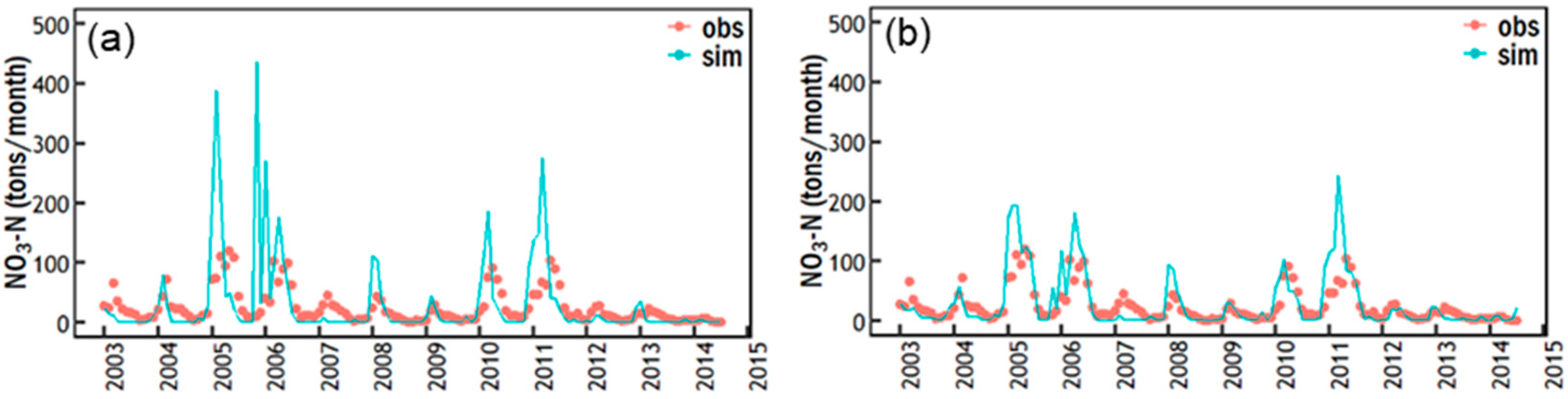
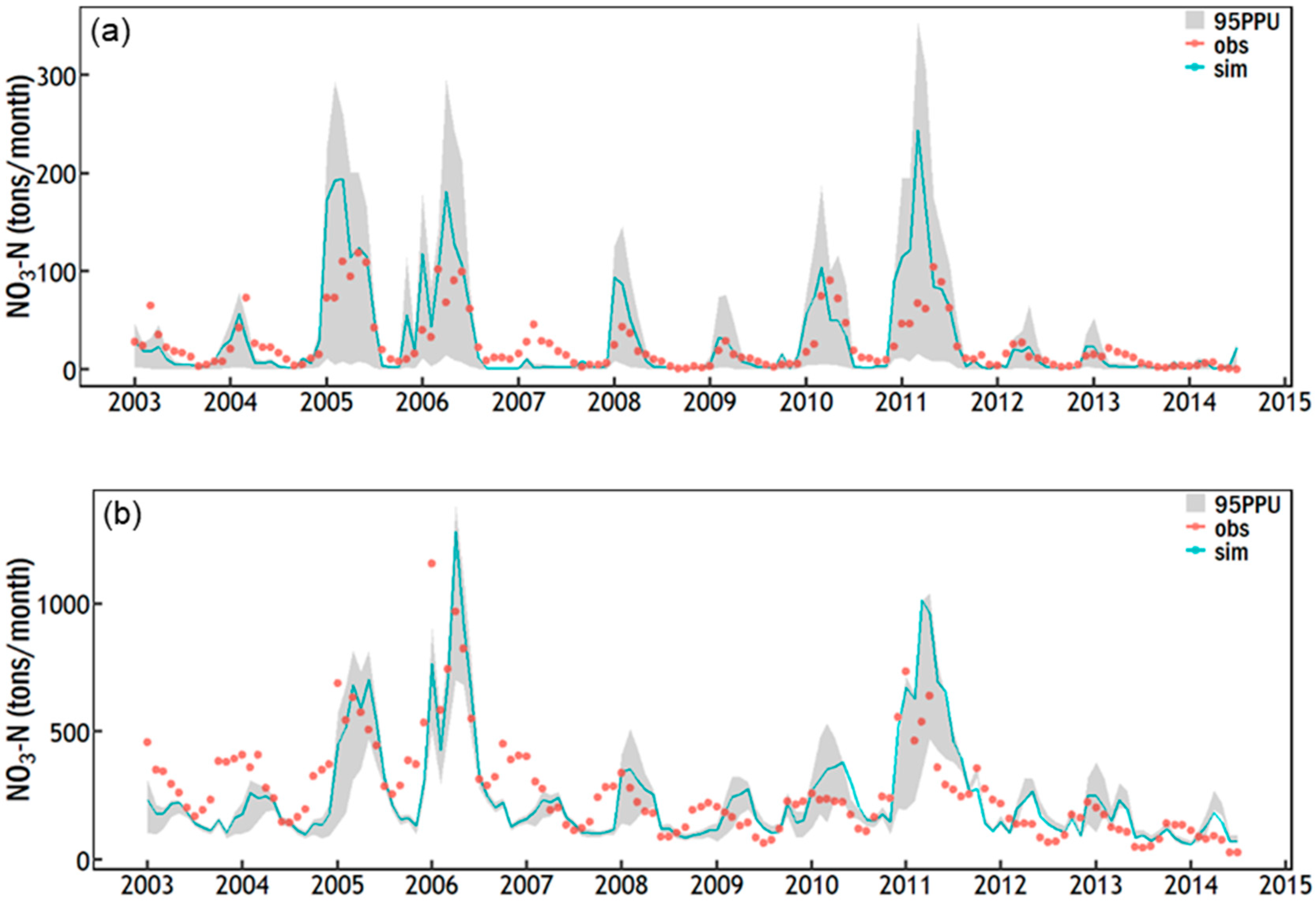
3.3. Simulation of Riverine Nitrate Loads

According to the model simulation, an average of 3135 tons of nitrate were exported annually through the San Joaquin River near the Vernalis outlet over the study period (Figure 3). Annual nitrate loads at the Vernalis outlet ranged from 1657 tons/year in 2013 to 6283 tons/year in 2006. The 95 PPU band (shaded area in Figure 3) was calculated based on the final parameter ranges presented in Table 3. For the San Joaquin River at Fremont Ford Bridge, the 95 PPU band bracketed 56% and 67% of the measured data during calibration and validation, respectively (Table 4). For the San Joaquin River near Vernalis, more than 50% of the measurements were captured by the 95 PPU. The average values for the R-factor were 0.74 and 1.77 for the Vernalis and Fremont stations, respectively. For deterministic simulations, nitrate simulation results were rated as at least “satisfactory” based on R2 and PBIAS during the calibration and validation periods at both stations. In particular, the performance rating was at least “satisfactory” according to all three metrics during the calibration period at the watershed outlet. NSE ratings were consistently lower as compared to the other two metrics. Illustrations of the observed and simulated nitrate loads indicate that some peak nitrate loads were overestimated, especially at the Fremont station (Figure 3). The poor performance in NSE is caused by the mismatch of peaks in 2005 and 2011. Since NSE computes the differences between the observation and simulation as square values (Table 2), it is sensitive to peak values [73]. However, SWAT still tracked the monthly nitrate loadings in the San Joaquin River reasonably well for other months.

4. Discussion

4.1. Tile Drainage Simulation

The default tile drainage routine calculates drainage flow timing based on only one parameter, TDRAIN (time to drain soils to field capacity). This method does not differentiate TDRAIN between large storms and small events [34]. The alternate tile drainage routine in SWAT incorporates the more physically based Hooghoudt and Kirkham tile drain equations, instead of a simple parameter TDRAIN. It also incorporates a drainage coefficient that limits the possible drainage volume in 24 h, therefore reducing the allowed maximal nitrate loading rates. The alternate tile drainage routine changes the shape of the nitrate runoff hydrograph. In that way, the pollutographs with abrupt peaks are altered to ones with smooth, more widely spread “bumps” (Figure 2). As a result, model predictions compared fairly well with the observed data. Our results show that the physically based Hooghoudt and Kirkham tile drain equations together with a drainage coefficient are able to reliably predict nitrate losses delivered by tile drains. No significant differences in the predicted streamflow compared to the measured values were found between the original and alternate tile drainage routines. This result occurs because the flow volume at the Fremont Ford Bridge is heavily dependent on upstream reservoir releases [24]. As a result, tile drainage has little impact on the overall streamflow trends.
We found that about 40% of the simulated nitrate losses were from tile nitrate in the San Joaquin River watershed over the study period. This finding is consistent with our knowledge that tile drains are critical for nitrate movement in surface water within the San Joaquin River watershed [14]. Results from a previous study suggested that tile drainage contributed 22% of the total nitrogen loads in the San Joaquin River at Vernalis for the years 1985 to 2004 [38]. This percentage was derived from measured nitrogen loads and a methodology for estimating tile drain discharge and concentrations [39]. Since total nitrogen is the sum of nitrate-nitrogen, nitrite-nitrogen, ammonia-nitrogen, and organic nitrogen, we consider our estimates comparable to the previous study.

4.2. Simulation of Riverine Nitrate Loads

In general, monthly nitrate loads in the San Joaquin River were well captured by SWAT, except for the overestimation of peak loads at the Fremont station (Figure 3). As a result, NSE showed less correspondence between observed and simulated values (Table 4), despite R2 and PBIAS ratings of at least “satisfactory” that indicated both strong linear relationships between the observed and simulated loads and low average model simulation bias (over- vs. under-estimation). One of the major disadvantages of NSE is its sensitivity to large values in a time series [68]. Therefore, overestimation of peak loads is likely to lead to poor NSE performance ratings.
In hydrologic modeling, uncertainties in predicted output may arise from model structure, model parameters, and spatial and temporal variability in the input data [64,74]. SUFI-2 maps all parameter uncertainty sources and aims to achieve the smallest range of parameter uncertainty while bracketing most of the measurements in the 95 PPU band. These two aspects were quantified by the P-factor, which measures to what extent model uncertainties are being considered, and the R-factor, which indicates the strength of calibration [66]. Results from uncertainty analysis indicate that there was a balance between uncertainty measures and the strength of calibration (Table 4). Although the R-factor was slightly greater than the desired value of 1, we did not continue to refine the uncertainty analysis because a further decrease in the parameter ranges would lead to a P-factor of less than 0.5.
In this study, the major sources of uncertainty in nitrogen simulation include the lack of information about the rate and date of fertilizer and manure application at the HRU level. Fertilization application rates and timing vary among regions and growers, depending on weather patterns, water availability, crop prices, yield goals, etc. (M. Lundy, personal communication, March 2017). Uncertainty also exists in manure application rates and areas. Manure generated by confined animal feeding operations is typically applied to adjacent forage cropland. Application rates are dictated by a variety of factors, including the capacity of the manure storage pond and the type of crop [54]. In preparing the nitrogen input data, we used average nitrogen application rates and a single schedule. We also assumed that a fixed portion of the nitrogen input was derived from manure for forage crops. While such simplifications do not strictly represent the actual distribution of nitrogen inputs across the San Joaquin River watershed, the general lack of explicit fertilizer and manure application data requires the use of a simplified, standard nitrogen management routine. Such approximations are frequently adopted in nutrient modeling [19,75,76,77,78]. Previous studies [14,79,80] derived estimates of nitrogen inputs in the San Joaquin River watershed from reports compiled by USGS in support of its National Water-Quality Program (NWQP) [2,81,82]. These data are too coarse for our modeling purposes, since they are annual county-level estimates. There is clearly a need for better estimates of fertilizer and manure application data with improved spatial and temporal resolution in intensive nutrient input areas, such as the San Joaquin River watershed.

4.3. Riverine Nitrate Exports, Aquatic Weed Infestation, and Future Climate Change Impact

The San Joaquin River plays a critical role in exporting nitrogen to the Delta, as 3135 tons of nitrate were exported annually through the Vernalis outlet (Figure 3). Loading from the San Joaquin River is particularly important during the summer months when the San Joaquin River watershed contributed 50% of the total nitrogen loading to the Delta [38]. Results in this study demonstrate the impacts of tile drainage on nitrogen loading in the San Joaquin River watershed. Therefore, conservation practices for reducing tile nitrate loss could be helpful in mitigating aquatic weed infestations in the Delta. For example, previous research shows that a controlled drainage system, which contains moveable flash boards to control the subsurface water table, is reliable for reducing nitrate loss through tile drains [83].
River nutrient inputs are one of the major drivers of the summertime growth of invasive aquatic vegetation, especially floating aquatic vegetation like water hyacinth, which obtains nutrients primarily from the water column. In general, increasing nitrogen levels lead to increases in biomass and density of aquatic macrophytes [3,84]. However, the relative contribution of nutrients in facilitating the growth and spread of invasive aquatic vegetation is not well understood, especially in the context of the complex Delta ecosystem [3]. Ongoing efforts to understand the response mechanisms of invasive aquatic weeds to nutrient inputs include the development of aquatic weed growth models [7,85]. Responses to nitrogen, as well as other limiting factors, such as temperature and light, are explicitly defined based on data collected in lab and field experiments. Simulated nitrogen loadings and concentrations from the outlet of the San Joaquin river basin could support aquatic weed growth models with important water quality parameters, such as nitrate loading to the Delta.
Climate change in the study region indicates a drier tendency with higher temperature and lower precipitation [86], which reduces snowpack in the eastern mountain region, and hence reduces the water storage in the state and Federal reservoirs [87]. Brekke, et al. [88] evaluated the potential climate change impacts on regional water resources in the San Joaquin river basin. Streamflow shifts in both the amount and timing are predicted by the CalSim model [89]. A generalized tendency of decreased reservoir inflows with earlier peaks in the eastern San Joaquin region is expected, indicating substantial impacts on the operation and planning of water resources, especially irrigated agriculture with heavy reliance on released reservoir water. This tendency will produce adverse effects on water quality, especially water salinity and nitrate concentration. For example, reduced water deliveries to the west agricultural regions from reservoirs encourage water reuse and groundwater exploitation, resulting in tailwater and tile drainage with higher concentrations of salts and nitrates conveyed to the San Joaquin River, eventually draining to the Bay-Delta Estuary.
Historical observation records already indicate upward trends of nitrate concentrations in the San Joaquin river basin. For example, nitrate concentration has increased from 1 mg/L to around 1.4 mg/L from 1975 to 2004 near Vernalis. For a specific monitoring site (Mud Slough) at western agricultural region, the increasing trend is as high as 493% [38]. Drier and warmer climates in the future has potentials to accelerate this increasing trend in San Joaquin water ways, facilitating the rapid growth of water hyacinth, especially under warmer conditions [90]. Previous studies indicated that higher density and rapid growth rates (10 kg/m2 in 50 days) are predicted for water hyacinth in a eutrophic environment (dissolved nitrogen more than 1 mg/L) under warm conditions (30 °C) [91].
Additional modeling efforts are still required to characterize the fate and transport of nitrogen within the Delta [7,92]. In the future, coupling watershed and Delta models with aquatic weed growth models would allow us to explore the impact of agricultural nitrogen loading on the downstream aquatic environment. The coupled model could be used to assess alternative agricultural management practices and climate scenarios (e.g., drought) [6,93,94,95,96], leading to proactive management strategies for aquatic weed control.

5. Conclusions

In this study, we used the SWAT model to investigate nitrogen exports from the San Joaquin River watershed to Bay-Delta, California. We evaluated the tile drain routines of SWAT and found that the more physically based Hooghoudt and Kirkham tile drain equations, and the inclusion of a drainage coefficient, better represent the measured nitrate loads. Simulations suggested that 40% of nitrate loading to the San Joaquin River came from tile nitrate, consistent with previous studies, which showed that tile drains are important for nitrate delivery in the San Joaquin River watershed. SWAT tracked the monthly riverine nitrate dynamics reasonably well, given the uncertainty in the nutrient management data. More accurate and consistent data on nitrogen use at finer temporal and spatial resolutions are clearly needed. The San Joaquin River plays an important role in supplying nitrogen to the Bay-Delta by exporting 3135 tons of nitrate-nitrogen annually, which is an important nutrient source for aquatic weed growth. Future climate change indicated an increasing trend of nitrate concentration exported from San Joaquin river basin, which facilitates the rapid growth of water hyacinth under warmer conditions, leading to a more severe infestation situation in the Bay-Delta waterways. Our modeling results could be further used to drive downstream aquatic weed growth models to assess the relative importance of nutrient loading on aquatic weed growth, potentially yielding insights into sustainable management practices for improved weed control.

Author Contributions

Conceptualization, R.W., H.C., and M.Z.; methodology, H.C. and M.Z.; software, H.C. and Y.L.; validation, R.W., and M.Z.; formal analysis, R.W. and H.C.; investigation, R.W., H.C., Y.L., and M.Z.; resources, Y.L. and P.M.; data curation, H.C. and Y.L.; writing—original draft preparation, H.C. and R.W.; writing—review and editing, R.W., H.C., M.Z., P.M., and M.G.; visualization, H.C. and R.W.; supervision, M.Z. and P.M.; project administration, M.Z. and P.M.; funding acquisition, P.M.

Funding

This research was funded by the USDA Delta Region Areawide Aquatic Weed Project (DRAAWP), grant number 58-2030-6-042.

Acknowledgments

This material is based upon work supported by the Delta Stewardship Council Delta Science Program under Grant No. 2271. We also wish to acknowledge support from the USDA-ARS Delta Region Areawide Aquatic Weed Project (DRAAWP) and the National Aeronautics and Space Administration, Ames Research Center. We are grateful to Brenna J. Aegerter, Brian Marsh, Daniel S. Munk, Mark Battany, Mark Lundy, and Marsha L Campbell from University of California Cooperative Extension for providing very helpful information on nutrient management practices in the San Joaquin River watershed.

Conflicts of Interest

The authors declare no conflict of interest.

References

  1. Galloway, J.N.; Townsend, A.R.; Erisman, J.W.; Bekunda, M.; Cai, Z.; Freney, J.R.; Martinelli, L.A.; Seitzinger, S.P.; Sutton, M.A. Transformation of the nitrogen cycle: Recent trends, questions, and potential solutions. Science 2008, 320, 889–892. [Google Scholar] [CrossRef]
  2. Ruddy, B.C.; Lorenz, D.L.; Mueller, D.K. County-Level Estimates of Nutrient Inputs to the Land Surface of the Conterminous United States, 1982–2001; 2006-5012; US Geological Survey: Reston, VA, USA, 2006.
  3. Dahm, C.N.; Parker, A.E.; Adelson, A.E.; Christman, M.A.; Bergamaschi, B.A. Nutrient dynamics of the Delta: Effects on primary producers. San Franc. Estuary Watershed Sci. 2016, 14. [Google Scholar] [CrossRef]
  4. Glibert, P.M.; Fullerton, D.; Burkholder, J.M.; Cornwell, J.C.; Kana, T.M. Ecological stoichiometry, biogeochemical cycling, invasive species, and aquatic food webs: San Francisco Estuary and comparative systems. Rev. Fish. Sci. 2011, 19, 358–417. [Google Scholar] [CrossRef]
  5. Seitzinger, S.; Lee, R.Y. Land-based nutrient loading to LMEs: A global watershed perspective on magnitudes and sources. Environ. Dev. 2016, 17, 220–229. [Google Scholar]
  6. Yuan, Y.; Wang, R.; Cooter, E.; Ran, L.; Daggupati, P.; Yang, D.; Srinivasan, R.; Jalowska, A. Integrating multimedia models to assess nitrogen losses from the Mississippi River basin to the Gulf of Mexico. Biogeosciences 2018, 15, 7059–7076. [Google Scholar] [CrossRef]
  7. Kyser, G.B.; Moran, P.J.; Madsen, J.D.; Pratt, P.D.; Bubenheim, D.L.; Hard, E.; Zhang, M.; Lawler, S.P.; Jetter, K.; Stanton, B.; et al. Delta Region Areawide Aquatic Weed Project Website. Available online: http://www.ucanr.edu/sites/DRAAWP/ (accessed on 17 May 2019).
  8. Luo, Y.; Zhang, X.; Liu, X.; Ficklin, D.; Zhang, M. Dynamic modeling of organophosphate pesticide load in surface water in the northern San Joaquin Valley watershed of California. Environ. Pollut. 2008, 156, 1171–1181. [Google Scholar] [CrossRef]
  9. Connolly, R.D.; Kennedy, I.R.; Silburn, D.M.; Simpson, B.W.; Freebairn, D.M. Simulating endosulfan transport in runoff from cotton fields in Australia with the GLEAMS model. J. Environ. Qual. 2001, 30, 702–713. [Google Scholar] [CrossRef] [PubMed]
  10. Fohrer, N.; Dietrich, A.; Kolychalow, O.; Ulrich, U. Assessment of the Environmental Fate of the Herbicides Flufenacet and Metazachlor with the SWAT Model. J. Environ. Qual. 2014, 43, 75–85. [Google Scholar] [CrossRef] [PubMed]
  11. Wang, R.; Yuan, Y.; Yen, H.; Grieneisen, M.; Arnold, J.; Wang, D.; Wang, C.; Zhang, M. A review of pesticide fate and transport simulation at watershed level using SWAT: Current status and research concerns. Sci. Total Environ. 2019, 669, 512–526. [Google Scholar] [CrossRef]
  12. Yen, H.; Lu, S.; Feng, Q.; Wang, R.; Gao, J.; Brady, D.M.; Sharifi, A.; Ahn, J.; Chen, S.-T.; Jeong, J. Assessment of optional sediment transport functions via the complex watershed simulation model SWAT. Water 2017, 9, 76. [Google Scholar] [CrossRef]
  13. Wang, R.; Chen, H.; Luo, Y.; Yen, H.; Arnold, J.G.; Bubenheim, D.; Moran, P.; Zhang, M. Modeling Pesticide Fate and Transport at Watershed Scale Using the Soil & Water Assessment Tool: General Applications and Mitigation Strategies. In Pesticides in Surface Water: Monitoring, Modeling, Risk Assessment, and Management; American Chemical Society: Washington, DC, USA, 2019; Volume 1308, pp. 391–419. [Google Scholar]
  14. Saleh, D.; Domagalski, J. SPARROW modeling of nitrogen sources and transport in rivers and streams of California and adjacent states, U.S. J. Am. Water Resour. Assoc. 2015, 51, 1487–1507. [Google Scholar] [CrossRef]
  15. Chen, H.; Zhan, Y.; Grieneisen, M.L.; Zhang, M. Spatio-Temporal Analyses of Pesticide Use on Walnuts and Potential Risks to Surface Water in California. In Managing and Analyzing Pesticide Use Data for Pest Management, Environmental Monitoring, Public Health, and Public Policy; Zhang, M., Jackson, S., Robertson, M.A., Zeiss, M.R., Eds.; American Chemical Society: Washington, DC, USA, 2018; Volume 1283, pp. 171–201. [Google Scholar]
  16. Wang, R.; Luo, Y.; Chen, H.; Yuan, Y.; Bingner, R.L.; Denton, D.; Locke, M.; Zhang, M. Environmental fate and impact assessment of thiobencarb application in California rice fields using RICEWQ. Sci. Total Environ. 2019, 664, 669–682. [Google Scholar] [CrossRef] [PubMed]
  17. Niraula, R.; Kalin, L.; Wang, R.; Srivastava, P. Determining Nutrient and Sediment Critical Source Areas with Swat: Effect of Lumped Calibration. Trans. ASABE 2012, 55, 137–147. [Google Scholar] [CrossRef]
  18. Arnold, J.G.; White, M.J.; Harmel, R.D.; Moriasi, D.N.; Gassman, P.W.; Abbaspour, K.C.; Srinivasan, R.; Santhi, C.; Kannan, N.; Van Griensven, A.; et al. SWAT: Model use, calibration, and validation. Trans. ASABE 2012, 55, 1491–1508. [Google Scholar] [CrossRef]
  19. Jha, M.K.; Gassman, P.W.; Arnold, J.G. Water quality modeling for the Raccoon River watershed using SWAT. Trans. ASABE 2007, 50, 479–493. [Google Scholar] [CrossRef]
  20. Ficklin, D.L.; Luo, Y.; Zhang, M. Climate change sensitivity assessment of streamflow and agricultural pollutant transport in California’s Central Valley using Latin hypercube sampling. Hydrol. Process. 2013, 27, 2666–2675. [Google Scholar] [CrossRef]
  21. Guo, T.; Gitau, M.; Merwade, V.; Arnold, J.; Srinivasan, R.; Hirschi, M.; Engel, B. Comparison of performance of tile drainage routines in SWAT 2009 and 2012 in an extensively tile-drained watershed in the Midwest. Hydrol. Earth Syst. Sci. 2018, 22, 89–110. [Google Scholar] [CrossRef]
  22. Boithias, L.; Srinivasan, R.; Sauvage, S.; Macary, F.; Sánchez-Pérez, J.M. Daily Nitrate Losses: Implication on Long-Term River Quality in an Intensive Agricultural Catchment of Southwestern France. J. Environ. Qual. 2014, 43, 46–54. [Google Scholar] [CrossRef] [PubMed]
  23. Hu, X.; McIsaac, G.F.; David, M.B.; Louwers, C.A.L. Modeling riverine nitrate export from an East-Central Illinois watershed using SWAT. J. Environ. Qual. 2007, 36, 996–1005. [Google Scholar] [CrossRef]
  24. Chen, H.; Luo, Y.; Potter, C.; Moran, P.J.; Grieneisen, M.L.; Zhang, M. Modeling pesticide diuron loading from the San Joaquin watershed into the Sacramento-San Joaquin Delta using SWAT. Water Res. 2017, 121, 374–385. [Google Scholar] [CrossRef]
  25. Quinn, N.W. The San Joaquin Valley: Salinity and drainage problems and the framework for a response. In Salinity and Drainage in San Joaquin Valley, California; Springer: Berlin, Germany, 2014; pp. 47–97. [Google Scholar]
  26. Quinn, N.W.T. Adaptive implementation of information technology for real-time, basin-scale salinity management in the San Joaquin Basin, USA and Hunter River Basin, Australia. Agric. Water Manag. 2011, 98, 930–940. [Google Scholar] [CrossRef]
  27. Capel, P.D.; McCarthy, K.A.; Barbash, J.E. National, Holistic, Watershed-Scale Approach to Understand the Sources, Transport, and Fate of Agricultural Chemicals. J. Environ. Qual. 2008, 37, 983–993. [Google Scholar] [CrossRef]
  28. Saleh, D.K.; Kratzer, C.R.; Green, C.H.; Evans, D.G. Using the Soil and Water Assessment Tool (SWAT) to Simulate Runoff in Mustang Creek Basin, California; US. Geological Survey: Reston, VA, USA, 2009.
  29. Dubrovsky, N.M. Water Quality in the San Joaquin-Tulare Basins, California; 1992–1995; US Geological Survey: Reston, VA, USA, 1998; Volume 1159.
  30. Wang, R.Y.; Bowling, L.C.; Cherkauer, K.A. Estimation of the effects of climate variability on crop yield in the Midwest USA. Agric. For. Meteorol. 2016, 216, 141–156. [Google Scholar] [CrossRef]
  31. Guo, T.; Cibin, R.; Chaubey, I.; Gitau, M.; Arnold, J.G.; Srinivasan, R.; Kiniry, J.R.; Engel, B.A. Evaluation of bioenergy crop growth and the impacts of bioenergy crops on streamflow, tile drain flow and nutrient losses in an extensively tile-drained watershed using SWAT. Sci. Total Environ. 2018, 613, 724–735. [Google Scholar] [CrossRef]
  32. Moriasi, D.N.; Rossi, C.G.; Arnold, J.G.; Tomer, M.D. Evaluating hydrology of the Soil and Water Assessment Tool (SWAT) with new tile drain equations. J. Soil Water Conserv. 2012, 67, 513–524. [Google Scholar] [CrossRef]
  33. Moriasi, D.N.; Gowda, P.H.; Arnold, J.G.; Mulla, D.J.; Ale, S.; Steiner, J.L.; Tomer, M.D. Evaluation of the Hooghoudt and Kirkham tile drain equations in the Soil and Water Assessment Tool to simulate tile flow and nitrate-nitrogen. J. Environ. Qual. 2014, 42, 1699–1710. [Google Scholar] [CrossRef]
  34. Boles, C.M.; Frankenberger, J.R.; Moriasi, D.N. Tile drainage simulation in SWAT2012: Parameterization and evaluation in an Indiana watershed. Trans. ASABE 2015, 58, 1201–1213. [Google Scholar]
  35. Lockhart, K.M.; King, A.M.; Harter, T. Identifying sources of groundwater nitrate contamination in a large alluvial groundwater basin with highly diversified intensive agricultural production. J. Contam. Hydrol. 2013, 151, 140–154. [Google Scholar] [CrossRef]
  36. USEPA. Region 9 Strategic Plan 2011–2014; Technical Report; United States Environmental Protection Agency: Washington, DC, USA, 2012.
  37. USDA-NASS. National Agricultural Statistics Service Cropland Data Layer. Available online: https://nassgeodata.gmu.edu/CropScape/ (accessed on 17 May 2019).
  38. Kratzer, C.R.; Kent, R.H.; Seleh, D.K.; Knifong, D.L.; Dileanis, P.D.; Orlando, J.L. Trends in Nutrient Concentrations, Loads, and Yields in Streams in the Sacramento, San Joaquin, and Santa Ana Basins, California 1975–2004; U.S. Geological Survey: Reston, VA, USA, 2011.
  39. Kratzer, C.R.; Shelton, J.L. Water Quality Assessment of the San Joaquin--Tulare Basins, California: Analysis of Available Data on Nutrients and Suspended Sediment in Surface Water 1972–1990; U.S. Dept. of the Interior, US Geological Survey: Reston, VA, USA, 1998.
  40. USGS. The National Map. Available online: http://nationalmap.gov/3dep_prodserv.html (accessed on 17 May 2019).
  41. USGS. National Hydrography Dataset (NHD). Available online: http://nhd.usgs.gov/data.html (accessed on 17 May 2019).
  42. Winchell, M.; Srinivasan, R.; Di Luzio, M.; Arnold, J. ArcSWAT interface for SWAT2012 User’s Guide; Blackland Research and Extension Center, Texas Agrilife Research; Grassland, Soil and Water Research Laboratory, USDA Agricultural Research Service: College Station, TX, USA, 2013.
  43. Fuka, D.R.; Walter, M.T.; MacAlister, C.; Degaetano, A.T.; Steenhuis, T.S.; Easton, Z.M. Using the Climate Forecast System Reanalysis as weather input data for watershed models. Hydrol. Process. 2013, 28, 5613–5623. [Google Scholar] [CrossRef]
  44. CDWR. California Irrigation Management Information System. Available online: http://www.cimis.water.ca.gov (accessed on 17 May 2019).
  45. USDA. Soil Survey Geographic (SSURGO) Database. Available online: http://sdmdataaccess.nrcs.usda.gov/ (accessed on 17 May 2019).
  46. Doll, D. Almond Nutrients & Fertilization. Available online: http://fruitsandnuts.ucdavis.edu/almondpages/AlmondNutrientsFertilization/ (accessed on 17 May 2019).
  47. CDFA. California Fertilization Guidelines. Available online: https://apps1.cdfa.ca.gov/fertilizerresearch/docs/guidelines.html (accessed on 17 May 2019).
  48. Peacock, B.; Christensen, P.; Hirschfelt, D. Best Management Practices for Nitrogen Fertilization of Grapevines; NG4-96; UC ANR: Davis, CA, USA, 1996. [Google Scholar]
  49. Hartz, T.; Miyao, G.; Mickler, J.; Lestrange, M.; Stoddard, S.; Nunez, J.; Aegerter, B. Processing Tomato Production in California; Publication No. 7228; UC ANR: Davis, CA, USA, 2008. [Google Scholar]
  50. Strange, M.L.; Schrader, W.L.; Hartz, T.K. Fresh-Market Tomato Production in California; Publication No. 8017; UC ANR: Davis, CA, USA, 2000. [Google Scholar]
  51. Ransom, J. Corn Growth and Management Quick Guide; NDSU Extension Service: Fargo, ND, USA, 2013. [Google Scholar]
  52. Geisseler, D.; Lazicki, P.A.; Pettygrove, G.S.; Ludwig, B.; Bachand, P.A.M.; Horwath, W.R. Nitrogen dynamics in irrigated forage systems fertilized with liquid dairy manure. Agron. J. 2012, 104, 897. [Google Scholar] [CrossRef]
  53. Munier, D.; Kearney, T.; Pettygrove, G.S.; Brittan, K.; Mathews, M.; Jackson, L. Small Grain Production Manual; Publication No. 8208; UC ANR: Davis, CA, USA, 2006. [Google Scholar]
  54. Harter, T.; Davis, H.; Mathews, M.C.; Meyer, R.D. Shallow groundwater quality on dairy farms with irrigated forage crops. J. Contam. Hydrol. 2002, 55, 287–315. [Google Scholar] [CrossRef]
  55. Sobota, D.J.; Harrison, J.A.; Dahlgren, R.A. Influences of climate, hydrology, and land use on input and export of nitrogen in California watersheds. Biogeochemistry 2009, 94, 43–62. [Google Scholar] [CrossRef]
  56. Chang, A.; Harter, T.; Letey, J.; Meyer, D.; Meyer, R.D.; Campbell, M.; Mitloehner, F.; Pettygrove, S.; Robinson, P.; Zhang, R. Groundwater Quality Protection: Managing Dairy Manure in the Central Valley of California; Publication No. 9004; UC ANR: Davis, CA, USA, 2007. [Google Scholar]
  57. NWQMC. Water Quality Portal (WQP). Available online: http://www.waterqualitydata.us/portal/ (accessed on 17 May 2019).
  58. State Water Board California Environmental Data Exchange Network (CEDEN). Available online: http://ceden.waterboards.ca.gov/AdvancedQueryTool (accessed on 17 May 2019).
  59. USGS rloadest: USGS Water science R Functions for LOAD ESTimation of constituents in rivers and Streams (version 0.4.4). Available online: https://github.com/USGS-R/rloadest (accessed on 17 May 2019).
  60. Wieczorek, M. Subsurface Drains on Agricultural Land in the Conterminous United States, 1992: National Resource Inventory Conservation Practice 606; U.S. Geological Survey: Reston, VA, USA, 2004.
  61. LSCE. Grassland Drainage Area Groundwater Quality Assessment Report; Luhdorff & Scalmanini, Consulting Engineers: Woodland, CA, USA, 2016. [Google Scholar]
  62. Arnold, J.G.; Kiniry, J.R.; Srinivasan, R.; Williams, J.R.; Haney, E.B.; Neitsch, S.L. Soil and Water Assessment Tool: Input/Output Documentation Version 2012; Texas Water Resources Institute: College Station, TX, USA, 2015. [Google Scholar]
  63. Abbaspour, K.C. SWAT-CUP: SWAT Calibration and Uncertainty Programs—A User Manual; Swiss Federal Institute of Aquatic Science and Technology: Dübendorf, Switzerland, 2015. [Google Scholar]
  64. Yen, H.; Wang, R.; Feng, Q.; Young, C.-C.; Chen, S.-T.; Tseng, W.-H.; Wolfe, J.E., III; White, M.J.; Arnold, J.G. Input uncertainty on watershed modeling: Evaluation of precipitation and air temperature data by latent variables using SWAT. Ecol. Eng. 2018, 122, 16–26. [Google Scholar] [CrossRef]
  65. Yen, H.; Wang, X.; Fontane, D.G.; Harmel, R.D.; Arabi, M. A framework for propagation of uncertainty contributed by parameterization, input data, model structure, and calibration/validation data in watershed modeling. Environ. Model. Softw. 2014, 54, 211–221. [Google Scholar] [CrossRef]
  66. Schuol, J.; Abbaspour, K.C.; Yang, H.; Srinivasan, R.; Zehnder, A.J.B. Modeling blue and green water availability in Africa. Water Resour. Res. 2008, 44. [Google Scholar] [CrossRef]
  67. Abbaspour, K.C.; Rouholahnejad, E.; Vaghefi, S.; Srinivasan, R.; Yang, H.; Kløve, B. A continental-scale hydrology and water quality model for Europe: Calibration and uncertainty of a high-resolution large-scale SWAT model. J. Hydrol. 2015, 524, 733–752. [Google Scholar] [CrossRef]
  68. Krause, P.; Boyle, D.P.; Bäse, F. Comparison of different efficiency criteria for hydrological model assessment. Adv. Geosci. 2005, 5, 89–97. [Google Scholar] [CrossRef]
  69. Moriasi, D.N.; Gitau, M.W.; Pai, N.; Daggupati, P. Hydrologic and water quality models: Performance measures and evaluation criteria. Trans. ASABE 2015, 58, 1763–1785. [Google Scholar]
  70. R Development Core Team R: A Language and Environment for Statistical Computing. Available online: https://www.r-project.org/ (accessed on 17 May 2019).
  71. Stringfellow, W.T.; Hanlon, J.S.; Borglin, S.E.; Quinn, N.W.T. Comparison of wetland and agriculture drainage as sources of biochemical oxygen demand to the San Joaquin River, California. Agric. Water Manag. 2008, 95, 527–538. [Google Scholar] [CrossRef]
  72. Neitsch, S.L.; Arnold, J.G.; Kiniry, J.R.; Williams, J.R. Soil and Water Assessment Tool Theoretical Documentation Version 2009; 406; Texas Water Resources Institute, Texas A&M University System: College Station, TX, USA, 2011. [Google Scholar]
  73. Legates, D.R.; McCabe, G.J., Jr. Evaluating the use of “goodness-of-fit” measures in hydrologic and hydroclimatic model validation. Water Resour. Res. 1999, 35, 233–241. [Google Scholar] [CrossRef]
  74. Guzman, J.A.; Shirmohammadi, A.; Sadeghi, A.M.; Wang, X.; Chu, M.L.; Jha, M.K.; Parajuli, P.B.; Harmel, R.D.; Khare, Y.P.; Hernandez, J.E. Uncertainty considerations in calibration and validation of hydrologic and water quality models. Trans. ASABE 2015, 58, 1745–1762. [Google Scholar]
  75. Zeiger, S.J.; Hubbart, J.A. A SWAT model validation of nested-scale contemporaneous stream flow, suspended sediment and nutrients from a multiple-land-use watershed of the central USA. Sci. Total Environ. 2016, 572, 232–243. [Google Scholar] [CrossRef]
  76. White, K.L.; Chaubey, I. Sensitivity analysis, calibration, and validations for a multisite and multivariable SWAT model. J. Am. Water Resour. Assoc. 2005, 41, 1077–1089. [Google Scholar] [CrossRef]
  77. Malagó, A.; Bouraoui, F.; Vigiak, O.; Grizzetti, B.; Pastori, M. Modelling water and nutrient fluxes in the Danube River Basin with SWAT. Sci. Total Environ. 2017, 603–604, 196–218. [Google Scholar] [CrossRef]
  78. Wang, R. Modeling Hydrologic and Water Quality Responses to Changing Climate and Land Use/Cover in the Wolf Bay Watershed, South Alabama; Auburn University: Auburn, AL, USA, 2010. [Google Scholar]
  79. Burow, K.R.; Shelton, J.L.; Dubrovsky, N.M. Regional nitrate and pesticide trends in ground water in the eastern San Joaquin Valley, California. J. Environ. Qual. 2008, 37, S249–S263. [Google Scholar] [CrossRef]
  80. Sobota, D.J.; Harrison, J.A.; Dahlgren, R.A. Linking dissolved and particulate phosphorus export in rivers draining California’s Central Valley with anthropogenic sources at the regional scale. J. Environ. Qual. 2011, 40, 1290–1302. [Google Scholar] [CrossRef]
  81. Gronberg, J.A.M.; Spahr, N.E. County-Level Estimates of Nitrogen and Phosphorus from Commercial Fertilizer for the Conterminous United States, 1987–2006; 2012-5207; US Geological Survey: Reston, VA, USA, 2012.
  82. Mueller, D.K.; Gronberg, J.A.M. County-Level Estimates of Nitrogen and Phosphorus from Animal Manure for the Conterminous United States, 2002; 2013-1065; US Geological Survey: Reston, VA, USA, 2013.
  83. Saadat, S.; Bowling, L.; Frankenberger, J.; Kladivko, E. Nitrate and phosphorus transport through subsurface drains under free and controlled drainage. Water Res. 2018, 142, 196–207. [Google Scholar] [CrossRef]
  84. You, W.; Yu, D.; Xie, D.; Yu, L.; Xiong, W.; Han, C. Responses of the invasive aquatic plant water hyacinth to altered nutrient levels under experimental warming in China. Aquat. Bot. 2014, 119, 51–56. [Google Scholar] [CrossRef]
  85. Boyer, K.; Sutula, M. Factors Controlling Submersed and Floating Macrophytes in the Sacramento-San Joaquin Delta; 870; Southern California Coastal Water Research Project: Costa Mesa, CA, USA, 2015. [Google Scholar]
  86. Ficklin, D.L.; Luo, Y.; Luedeling, E.; Gatzke, S.E.; Zhang, M. Sensitivity of agricultural runoff loads to rising levels of CO2 and climate change in the San Joaquin Valley watershed of California. Environ. Pollut. 2010, 158, 223–234. [Google Scholar] [CrossRef]
  87. Hidalgo, H.; Brekke, L.; Miller, N.; Quinn, N.; Keyantash, J.; Dracup, J. Assessment of the Impacts of Climate Change on the Water Allocation, Water Quality and Salmon Production in the San Joaquin River Basin. In Regional Climate Change and Variability: Impacts and Responses; Edward Elgar Pub: Cheltenham, UK, 2006; pp. 30–57. [Google Scholar]
  88. Brekke, L.D.; Miller, N.L.; Bashford, K.E.; Quinn, N.W.T.; Dracup, J.A. Climate Change Impacts Uncertainty for Water Resources in the San Joaquin River Basin, California. J. Am. Water Resour. Asso. 2004, 40, 149–164. [Google Scholar] [CrossRef]
  89. Draper, A.J.; Munévar, A.; Arora, S.K.; Reyes, E.; Parker, N.L.; Chung, F.I.; Peterson, L.E. CalSim: Generalized model for reservoir system analysis. J. Water Resour. Plan. Manag. 2004, 130, 480–489. [Google Scholar] [CrossRef]
  90. Heard, T.A.; Winterton, S.L. Interactions between nutrient status and weevil herbivory in the biological control of water hyacinth. J. Appl. Ecol. 2000, 37, 117–127. [Google Scholar] [CrossRef]
  91. Wilson, J.R.; Holst, N.; Rees, M. Determinants and patterns of population growth in water hyacinth. Aquat. Bot. 2005, 81, 51–67. [Google Scholar] [CrossRef]
  92. Novick, E.; Holleman, R.; Jabusch, T.; Sun, J.; Trowbridge, P.; Senn, D.; Guerin, M.; Kendall, C.; Young, M.; Peek, S. Characterizing and Quantifying Nutrient Sources, Sinks, and Transformations in the Delta: Synthesis, Modeling, and Recommendations for Monitoring; San Francisco Estuary Institute: Richmond, CA, USA, 2015. [Google Scholar]
  93. Wang, R.; Kalin, L. Combined and synergistic effects of climate change and urbanization on water quality in the Wolf Bay watershed, southern Alabama. J. Environ. Sci. 2018, 64, 107–121. [Google Scholar] [CrossRef] [PubMed]
  94. Ullrich, A.; Volk, M. Application of the Soil and Water Assessment Tool (SWAT) to predict the impact of alternative management practices on water quality and quantity. Agric. Water Manag. 2009, 96, 1207–1217. [Google Scholar] [CrossRef]
  95. Chen, J.; Liu, Y.; Gitau, M.W.; Engel, B.A.; Flanagan, D.C.; Harbor, J.M. Evaluation of the effectiveness of green infrastructure on hydrology and water quality in a combined sewer overflow community. Sci. Total Environ. 2019, 65, 69–79. [Google Scholar] [CrossRef]
  96. Gitau, M.W.; Chen, J.Q.; Ma, Z. Water Quality Indices as Tools for Decision Making and Management. Water Resour. Manag. 2016, 30, 2591–2610. [Google Scholar] [CrossRef]
Figure 1. Study area of the San Joaquin River watershed in California.
Sustainability 11 02845 g001
Figure 2. Observed (obs) and simulated (sim) monthly nitrate loads for the San Joaquin River at Fremont Ford Bridge using (a) the default tile drainage routine, and (b) the alternate tile drainage routine.
Sustainability 11 02845 g002
Figure 3. Observed (obs), simulated (sim), and the 95% prediction uncertainty (95 PPU) of monthly nitrate loads for the San Joaquin River (a) at Fremont Ford Bridge and (b) near Vernalis.
Sustainability 11 02845 g003
Table 1. Parameters for the original and alternate tile drainage routines of the Soil and Water Assessment Tool.
ParameterDescriptionValue
Parameters for the original tile drainage routine
ITDRN.bsnTile drainage equations flag0 = original,
1 = DRAINMOD
DDRAIN.mgtDepth to the subsurface drain (mm)1510
TDRAIN.mgtTime to drain soil to field capacity (h)24
GDRAIN.mgtDrain tile lag time (h)96
DEP_IMP.hruDepth to impervious layer in soil profile (mm)Approximated by depth to the bottom of the soil profile
Additional parameters for the alternate tile drainage routine
DRAIN_CO.sdrDaily drainage coefficient (mm/day)35
LATKSATF.sdrMultiplication factor to determine lateral ksat (conk(j1,j)) from SWAT ksat input value (sol_k(j1,j)) for HRU1
RE.sdrEffective radius of drains (mm)20
SDRAIN.sdrDistance between two drain tubes or tiles (mm)30,000
Table 2. Performance measures and associated performance evaluation criteria.
Performance RatingsNitrogen
R 2 = ( i = 1 n ( y i y ¯ ) ( y i ^ y ^ ¯ ) i = 1 n ( y i y ¯ ) 2 i = 1 n ( y i ^ y ^ ¯ ) 2 ) 2 NSE = 1 i = 1 n ( y i y i ^ ) 2 i = 1 n ( y i y ¯ ) 2 PPBIAS = i = 1 n ( y i ^ y i ) i = 1 n y i × 100   ( % )
Very good R 2 > 0.70 NSE > 0.65 | PBIAS | < 15
Good 0.60 < R 2 0.70 0.50 < NSE 0.65 15 | PBIAS | < 20
Satisfactory 0.30 < R 2 0.60 0.35 < NSE 0.50 20 | PBIAS | < 30
Unsatisfactory R 2 0.30 NSE 0.35 | PBIAS | 30
Note: y i and y i ^ are the ith observed and modeled values, y ¯ and y ^ ¯ is the average of the observed and modeled values, and n is the sample size.
Table 3. Sensitive parameters, calibrated ranges, and optimal values.
ParameterDescriptionLower LimitUpper LimitOptimal Value
CMN.bsnRate factor for humus mineralization of active organic nutrients (N and P)0.0001450.0002490.000169
CDN.bsnDenitrification exponential rate coefficient1.132.357197
SDNCO.bsnDenitrification threshold water content0.571.11.001510
NPERCO.bsnNitrate percolation coefficient00.20.176200
ANION_EXCL.solFraction of porosity from which anions are excluded0.010.790.446
HLIFE_NGW.gwHalf-life of nitrate in the shallow aquifer (days)3320090.870819
DEP_IMP.hruDepth to impervious layer in soil profile (m)061.23500
BC1.swqRate constant for biological oxidation of NH4 to NO2 (day−1)0.2110.909150
BC2.swqRate constant for biological oxidation of NO2 to NO3 (day−1)0.3721.789952
BC3.swqRate constant for hydrolysis of organic N to NH4 (day−1)0.240.40.267680
Table 4. Calibration and uncertainty analysis for monthly nitrate loads in the San Joaquin River watershed. NSE, Nash-Sutcliffe efficiency; PBIAS, percent bias.
StationP-FactorR-FactorR2R2 RatingNSENSE RatingPBIAS (%)PBIAS Rating
Calibration of nitrate simulation (2003–2008)
Vernalis0.530.630.68Good0.45Satisfactory−22Satisfactory
Fremont Ford Bridge0.561.720.67Good−0.11Unsatisfactory16Good
Validation of nitrate simulation (2009–2014)
Vernalis0.510.860.71Very good0.25Unsatisfactory24Satisfactory
Fremont Ford Bridge0.671.820.52Satisfactory−0.73Unsatisfactory29Satisfactory

