Article

Rapid Transit Systems: Smarter Urban Planning Using Big Data, In-Memory Computing, Deep Learning, and GPUs

1
Department of Computer Science, FCIT, King Abdulaziz University, Jeddah 21589, Saudi Arabia
2
High-Performance Computing Center, King Abdulaziz University, Jeddah 21589, Saudi Arabia
3
Faculty of Computing and Information Technology, Northern Border University, Rafha 91911, Saudi Arabia
*
Author to whom correspondence should be addressed.
Sustainability 2019, 11(10), 2736; https://doi.org/10.3390/su11102736
Submission received: 9 April 2019 / Revised: 4 May 2019 / Accepted: 4 May 2019 / Published: 14 May 2019
(This article belongs to the Special Issue Smart Mobility for Future Cities)

Abstract

:
Rapid transit systems or metros are a popular choice for high-capacity public transport in urban areas due to several advantages including safety, dependability, speed, cost, and lower risk of accidents. Existing studies on metros have not considered appropriate holistic urban transport models and integrated use of cutting-edge technologies. This paper proposes a comprehensive approach toward large-scale and faster prediction of metro system characteristics by employing the integration of four leading-edge technologies: big data, deep learning, in-memory computing, and Graphics Processing Units (GPUs). Using London Metro as a case study, and the Rolling Origin and Destination Survey (RODS) (real) dataset, we predict the number of passengers for six time intervals (a) using various access transport modes to reach the train stations (buses, walking, etc.); (b) using various egress modes to travel from the metro station to their next points of interest (PoIs); (c) traveling between different origin-destination (OD) pairs of stations; and (d) against the distance between the OD stations. The prediction allows better spatiotemporal planning of the whole urban transport system, including the metro subsystem, and its various access and egress modes. The paper contributes novel deep learning models, algorithms, implementation, analytics methodology, and software tool for analysis of metro systems.

1. Introduction

Train-based rapid transit systems—also known as tubes, underground, or metros—are a popular choice for high-capacity public transportation systems in urban areas. Rapid transit is used in urban areas typically for transporting large numbers of passengers over small distances, at high frequencies, and are usually preferred over other transportation modes due to its several advantages. Road transportation annually costs 1.25 million deaths and trillions of dollars to the global economy due to congestion [1,2]. Train-based rapid transit is the safest and most dependable mode of transportation due to lack of congestion, and a significantly lower chance of accidents and vehicle/system failure. It is the fastest forms of land transportation, is usually relatively inexpensive, and is good for economic and social sustainability.
Rapid transit systems are usually supported by other transportation modes such as trams, buses, ferries, vehicle park and ride stations, motorcycles, bike-sharing stations, and walking routes. Various topologies including lines, circle, grid and cross, are used for the railway structures. It is a complex system in itself due to an enormous number of passengers to be transported through a large number of stations connected through multiple train lines. Keeping track of the passengers, speedy issuance of tickets, enforcing the use of appropriate tickets, is one dimension of the system complexity. The routes need to be planned and the trains need to be scheduled in such a way to optimize passenger convenience and the overall throughput of the system. A more complex aspect of the rapid transit system design is to consider it a part of the larger urban transportation system, including complementary transportation resources and networks, and optimize it holistically, i.e., to consider the transportation routes and choices made by people, not only within the rapid transit system, but also outside the rapid transit, which includes, as mentioned before, trams, buses, bike-sharing stations, and walking routes. This optimization is a gigantic challenge, particularly if we consider cities such as London and its rapid transit, i.e., the London Metro, or the New York City Subway, Tokyo subway system, or the Beijing Subway. For brevity, from here on, we use “metro” to refer to rapid transit systems.
Many techniques have been proposed to model, analyze, and design metro systems. For instance, Hu et al. [3] develop an operation plan for intercity passenger train and the ticket prices using a multi-objective model. They apply their model to the intercity rail between the Chongqing and Chengdu cities. Sun et al. [4] provide an optimization method for train scheduling in a metro line including the terminal dwell time. The method, in optimizing the train schedule, takes into account the passenger preferences, plan robustness, and energy efficiency of the system. Escolano et al. [5] use artificial neural networks (ANNs) to optimize the bus scheduling and dispatch system in Metro Manila. The aim of the ANN model is to reduce passenger waiting time on the bus stops and hence reduce the overall journey time. Wang at al. [6] proposed two approaches for estimating train delays using historical and real-time data obtained from Amtrak US trains during 2011–2013.
Several researchers have tried to predict the number of passengers for metro systems using various techniques. Wang et al. [7] propose a prediction model to predict passenger volume combining Radial Basis Function (RBF) neural network and Least Squares Support Vector Machines (LSSVM). They use flow data of passengers traveling through the Dongzhimen subway stations from 2012. Abadi et al. [8] predict the number of train passengers in a selected region of Indonesia using a combination of a neuro-fuzzy model and singular value decomposition (SVD). Zhang et al. [9] design a skip-stop strategy to optimize the journey time and the number of passengers traveling in Shenzhen Metro. Zhao et al. [10] propose a probabilistic model to estimate the passenger flows through different trains and routes. The estimated passenger flows are useful in modeling passenger path choices. They use data from the Shenzhen Metro automated fare collection (AFC) system to evaluate their proposed technique. A detailed literature review of metro-based research is given in Section 2.
The focus of our research in this paper is to address the metro system performance using a holistic approach whereby the transportation authorities can optimize the performance of the whole urban transportation network. We have mentioned earlier that an urban transportation system usually includes one or more metro systems and the complementary transportation network which consists of other transportation modes, e.g., buses, ferries, and bike-sharing stations. The aim of the transportation authorities in an urban area is to provide public personalized, convenient, speedy, multi-modal, and inexpensive travel options. A transportation authority, such as a city council, for this purpose, builds transportation facilities for people to travel to the nearest metro stations from their homes, offices, or other Points of Interests (PoIs), and vice versa. The current works in this domain have not studied the performance of urban metro systems in such details.
Secondly, the use of cutting-edge technologies has been limited in these studies. The last few decades have seen an increasing surge in the technological advancements. The penetration of these technologies to all spheres of everyday life has given rise to the smart cities, smart societies, and smart infrastructure developments [11,12]; smart transportation infrastructure is at the forefront of these developments  [13,14,15]. The use of GPS devices and mobile signals to collect vehicle location and congestion data [16]; the use of big data [17,18,19,20] and high-performance computing (HPC) [17,19,21,22] technologies; mobile, cloud and fog computing [16,23,24,25,26]; image processing, deep learning, and artificial intelligence (AI) for road traffic analysis and prediction [27,28,29,30]; urban logistics prototyping [31]; vehicular ad hoc networks [24,32,33,34,35]; autonomous driving [27]; autonomic transportation systems [36,37,38]; and the use of social media for traffic event detection [39,40,41]; are but a few examples. There is a need for innovative uses of the cutting-edge technologies in transportation.
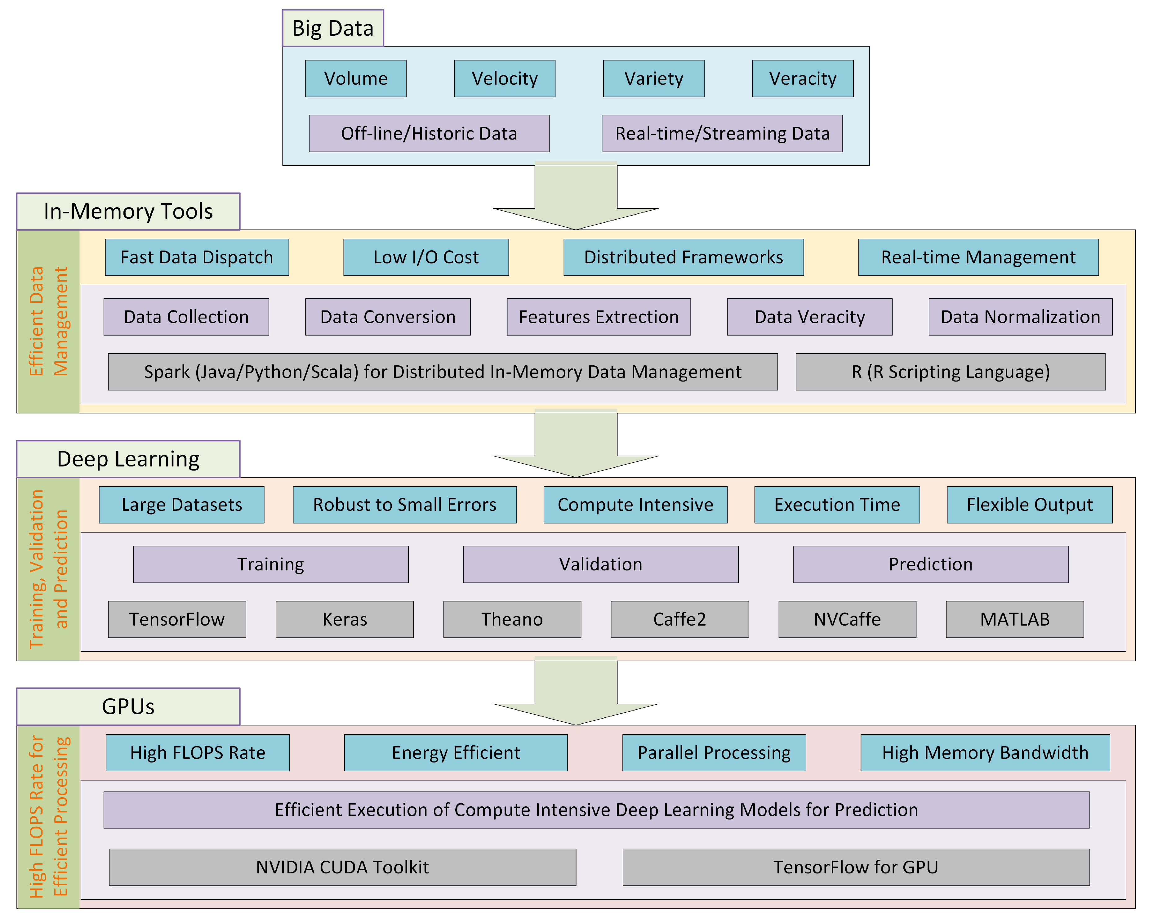
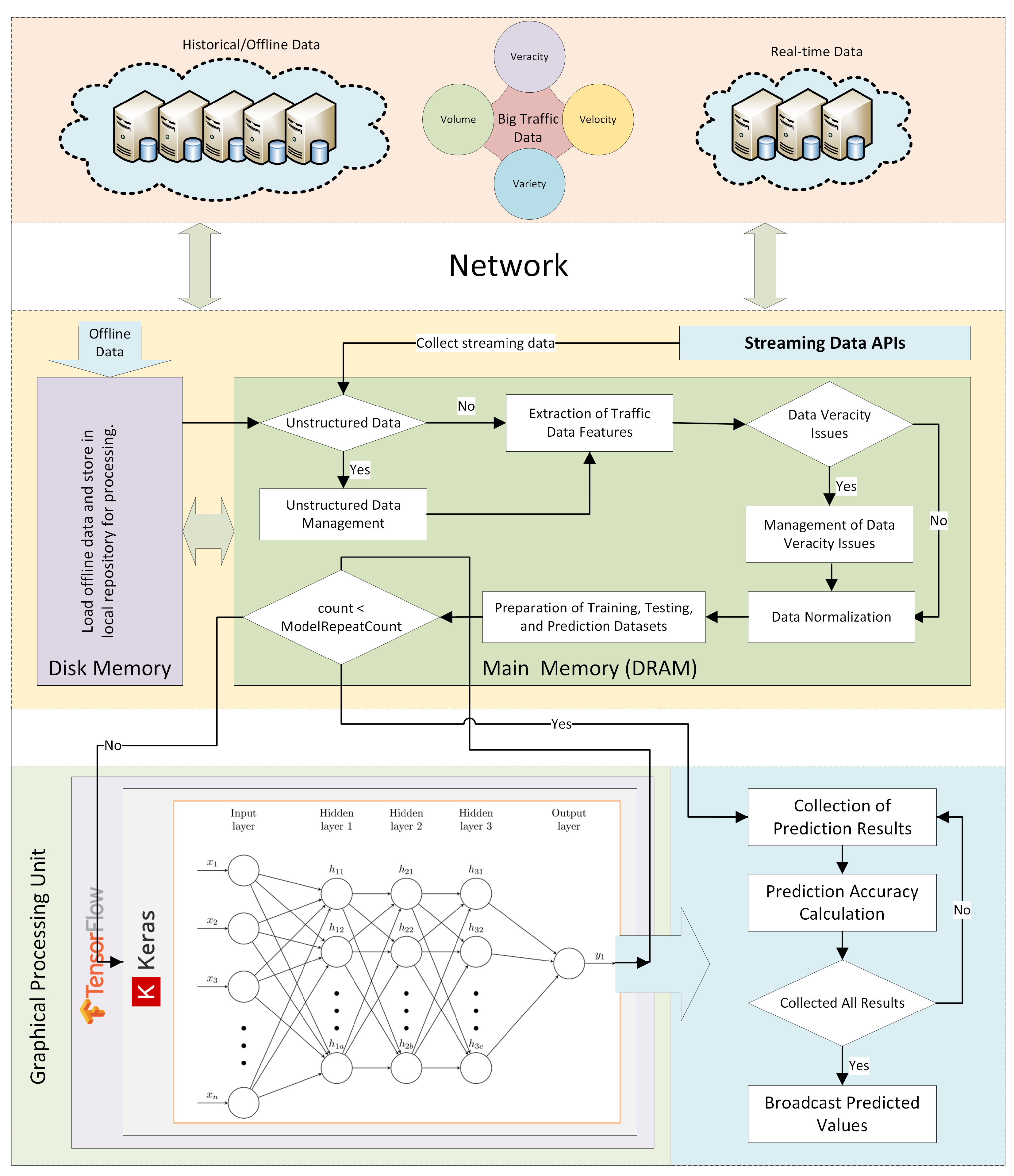
We focus on this paper on bringing four complementary cutting-edge technologies together—big data, in-memory computing, deep learning, and Graphics Processing Units (GPUs)—to address the challenges of holistically analyzing urban metro systems. The approach presented in this paper provides a novel and comprehensive approach toward large-scale urban metro systems analysis and design. GPUs provide massively parallel computing power to speed up computations. Big data leverages distributed and HPC technologies, such as GPUs, to manage and analyze data. Big data and HPC technologies are converging to address their individual limitations and exploit their synergies [42,43,44,45]. In-memory computing allows faster analysis of data using random-access memories (RAMs) as opposed to the secondary memories. Deep learning is used to predict various characteristics of urban metro systems.
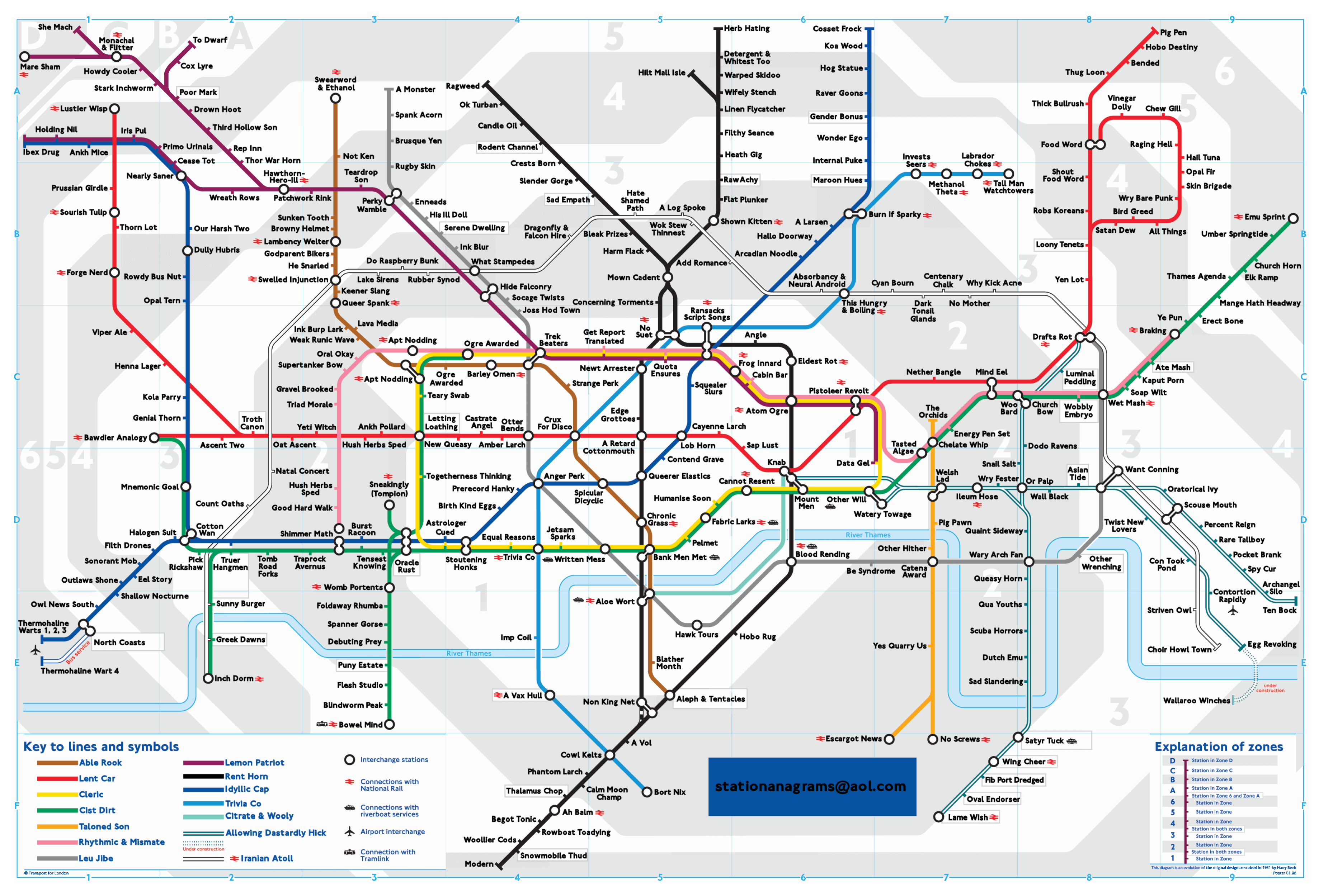
We have used the London Metro system as a case study in this paper to demonstrate the effectiveness of our proposed approach. The London Metro, also called London Underground, is one of the oldest rapid transit systems in the world, indeed the first metro system in the world. It has 270 stations and 11 train lines covering 402 KM, serving 5 million passenger journeys daily [46]. A map of the London Metro network is given in 
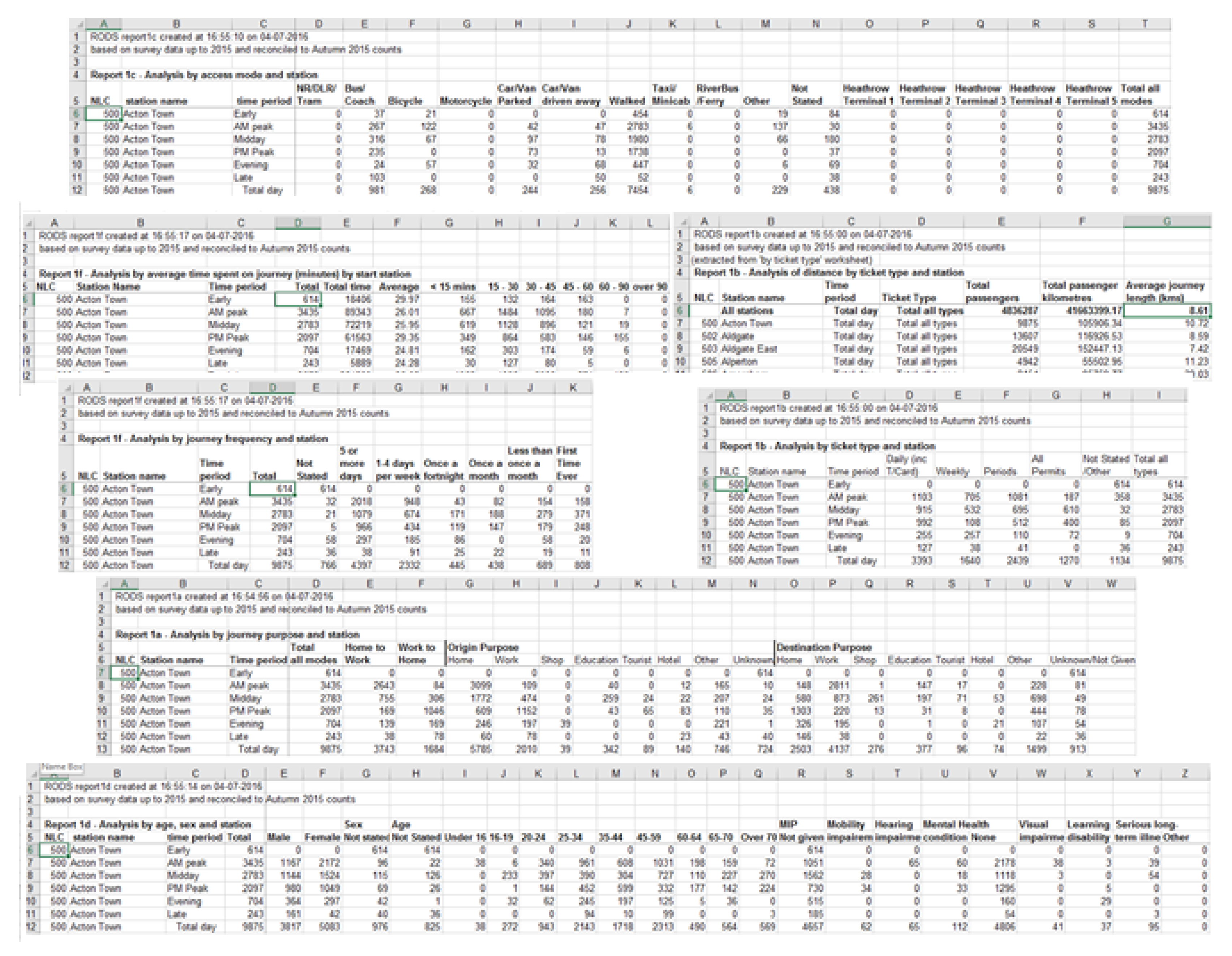
Figure 1. The dataset we have used in this study is provided by Transport for London (TFL) under the Rolling Origin and Destination Survey (RODS) program [47]. This data is collected by surveying the passengers traveling through the London Metro network in the United Kingdom. The purpose of this program is to collect the data of passengers traveling between different stations during different time intervals in a day. The data is available for the year 2015.
We use the RODS data to model the relationship between the number of passengers and (a) various access transportation modes used by the passengers to reach the train stations; (b) egress modes used to travel from the metro station to their next PoIs; (c) different origin-destination (OD) pairs of stations; and (d) the distance between the OD pairs of stations. Therefore, we predict, for six time intervals, the number of passengers using different access and egress modes to travel to, and travel from, each of the London Metro stations, respectively. We will see later in the paper that there are ten different types of access and egress transportation modes being used to complement the London Metro including buses and motorcycles. The information about the access and egress modes is valuable because it allows estimating the spatiotemporal use of various transportation modes, and could be used for planning and resource provisioning purposes. For example, if many passengers are using the access mode “car/van parked”, then the transportation authorities need to estimate whether the parking area reserved for the passengers to park their cars is sufficient to accommodate the vehicles. Similarly, the demand for buses and their time schedules could be estimated and planned for. We also predict for six time intervals the number of passengers that will be traveling between specific pairs of stations (OD pairs) at various time intervals, such as “PM Peak”. Moreover, we predict the number of passengers traveling between various OD station pairs to investigate the relationship between the number of passengers and the distance between those pairs of stations. This would be helpful in improving planning, resource provisioning, and quality of service of the urban transport system. This is the first study where the RODS data is used to model and predict various metro system characteristics.
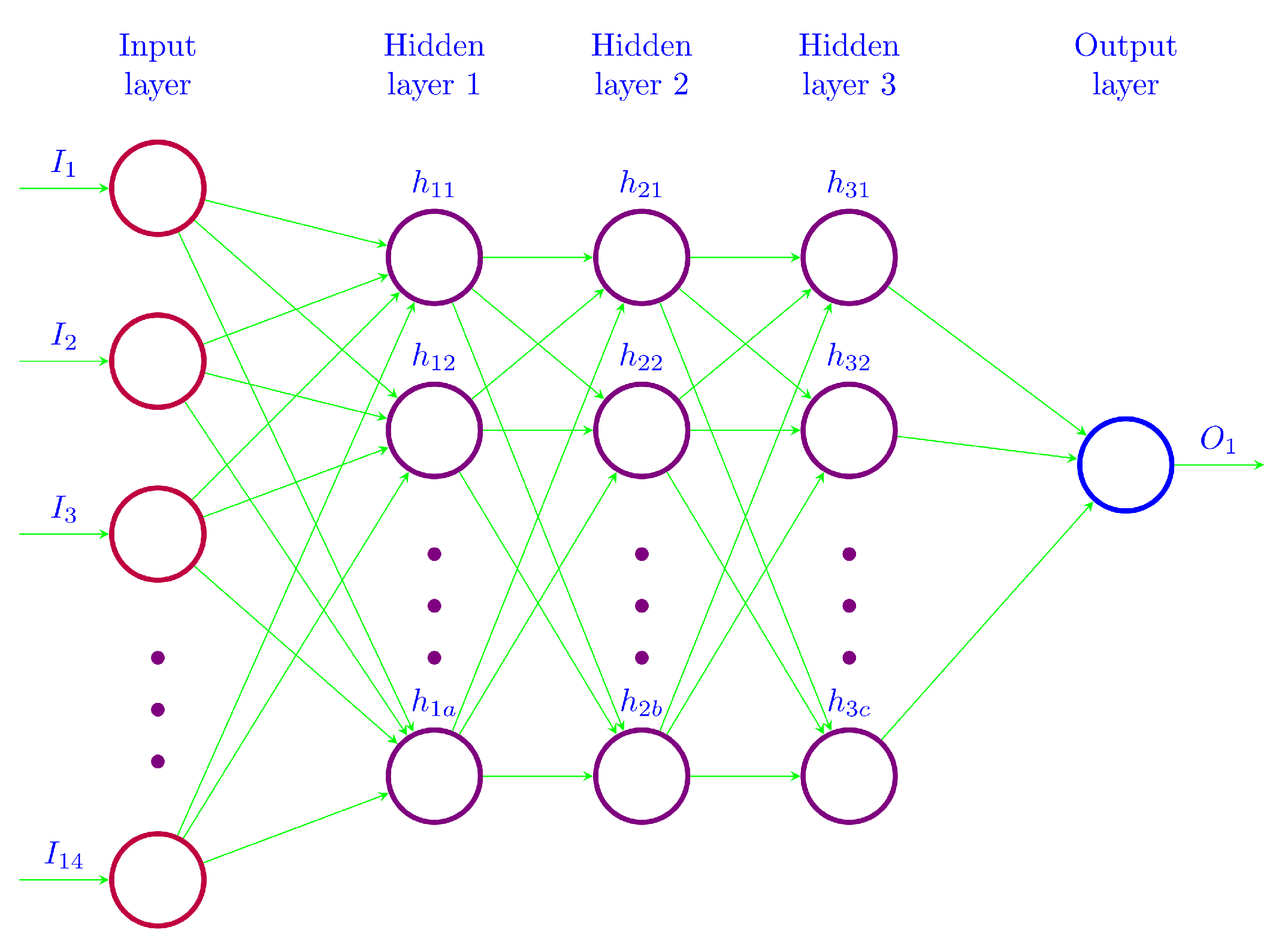
The RODS data described above is fed into the deep learning pipeline for training and prediction purposes. We have used Convolutional Neural Networks (CNNs) in our deep learning models. Firstly, the data is pre-processed to deal with the data veracity issues, and for data parsing and normalization. The data is processed in-memory using R [48] and Spark [49]. Subsequently, the data is fed to the deep learning engine, which is a compute intensive task. The use of GPUs provides a speedy deep learning training process. We have used two well-known evaluation metrics for the accuracy evaluation of our deep prediction models. These are mean absolute error (MAE) and mean absolute percentage error (MAPE). Additionally, we have provided the comparison of actual and predicted values of the metro characteristics. The results demonstrate a range of prediction accuracies, from high to fair. These are discussed in detail. The paper contributes novel deep learning models, algorithms, implementation, analytics methodology, and software tool for analysis of metro systems. The paper also serves as a preliminary investigation into the convergence of big data and HPC for the transportation sector, specifically for the rapid transit systems, incorporating London Metro as a case study. We would like to clarify here that HPC and big data convergence have been discussed by researchers in the literature for the last few years, such as in  [42,43,44,45]. We are not suggesting that this is the first study on the convergence in general, rather it is the first study on the convergence that focuses specifically on the transportation and rapid transit application domains. The topic of HPC and big data convergence is in its infancy and will require many more efforts by the community across diverse applications domains before reaching its maturity. We will explore these convergence issues in the future with the aim to devise novel multidisciplinary technologies for transportation and other sectors. This is the first study of its kind where integration of leading-edge technologies—big data, in-memory computing, deep learning, and HPC—have been applied to holistic modeling and prediction of a real rapid transit system.
The rest of the paper is organized as follows. The literature review is provided in Section 2. The proposed methodology is presented in Section 3. The analysis and results are given in Section 4. Section 5 concludes the paper and gives directions for future work.

2. Literature Review

This section provides a review of the works related to the main topics of this paper. Section 2.1 reviews the literature on rapid transit systems. Section 2.2 reviews the literature on deep learning approaches used in transport management.

2.1. Rapid Transit Systems

In [3], authors have proposed a model to determine the ticket price and the intercity operation plan to benefit both passengers and the transportation authorities. This will also beneficial in competition with the other modes of intercity transportation. Another study [4] proposes a method to prepare trains schedule and the trains dwell time at different stations keeping in mind the passengers demand on those stations. The purpose of model is to schedule the dwell time such that it should match with the number of passengers boarding and alighting the trains on those stations. The purpose of this optimization is to reduce the passengers waiting time and the operation costs and Lagrangian duality theory has been applied to find an optimal solution. Another similar work [50] provides a model and algorithm to solve the problems of both passengers and the railways authorities. It also provides a plan in accordance with the passenger flow and a software has been developed that implements the proposed algorithm to make optimal passenger train plans.
In addition to these approaches, a neural network-based approach for bus scheduling and dwell time has been proposed in [5]. Like [4], the aim of this study is also to reduce the waiting time for passengers on different stations. In the proposed model, authors have used a neural network with 10 hidden layers and a dataset of size 2430 samples. The dataset was divided into a ratio of 60%, 30%, and 10% for training, testing, and validation purposes, respectively. To evaluate the correctness of results, mean squared error has been used. Another approach to estimate the delays in train arrivals has been proposed by Ren Wang and Daniel B. Work in [6]. It uses a regression model to estimate the possible delay in train arrival on a specific station using a historical data. The data is collected for 282 trains in America during the period of 2011 to 2013. For analysis purpose, root mean squared error (RMSE) has been calculated.
An approach to estimate the possible route selection from passengers traveling through metro systems has been proposed in [10]. The authors in this article have used the information collected from the smart cards used for this service the provides the information about the origin, starting timestamp, destination, and end timestamp. To estimate the possible route selected by a passenger to travel from one point to other, they have used probabilistic model that can estimate the passenger flow in different trains in different routes by analyzing the historical data using OD tables. An approach to predict the number of passengers traveling through train by using neuro-fuzzy model with SVD has been proposed in [8]. They have used the historical data over a period from 2005 to 2011 that gives the monthly average number of passengers traveled through train. MAPE has been calculated to calculate the accuracy of results.
Similar work is done by Wang et al. in [7] to predict the number of passengers. They have used least squared support vector machines which uses one input, and a hidden and an output layer. Dataset used for training gives an average number of passengers on daily basis during 2012 and to calculate the accuracy of the system, mean average percentage error and mean squared error has been used. Ref. [9] proposes a train scheduling scheme using the skip-stop strategy to save both passengers travel time and the railway authority’s operation costs. For this purpose, a genetic algorithm has been applied on the data in the form of OD table. OD table is used here to find out the stations with high passengers’ flow as the stations with low flow rate could be skipped. To skip a station, some factors have been considered that include minimum headway, train capacity, and train operation to minimize average waiting time and operation costs.
Another study [51], investigates the role of model predictive control (MPC) for train regulations. In this study, authors have proposed a control law that could be used to optimize the metro system cost function by optimizing the upper bound on the cost function. According to them, the regulations are affected by uncertain passenger arrival and other kind of disturbances such as system failure etc. Proposed algorithm is implemented in MATLAB and some numerical examples are used for analysis purposes. The passengers flow on a particular station, including the number of passengers boarding, alighting, and waiting for train etc. effects the trains schedules and makes it complicated. The authors in [52] have proposed a model that evaluates the train schedule from the passengers’ perspective. For this purpose, they have used a time-driven microscopic model that considers all kind of passengers on stations. The dataset used for analysis purpose includes 634 trains and more than a million passengers.
An approach to understand the urban mobility (especially using trains in Singapore) is presented in [53]. The authors in this study have used the data generated by the farecards to travel through trains. The data generated by using the farecards provides the users’ id, origin, destination, stat time and, journey end time. To collect the data about the route to reach from the origin point to destination, geolocation data generated by the mobile devices has been used. To handle the geolocation data produced by mobile devices, IBM City in Motion (CiM) system has been used. CiM is built on Hadoop-based platform with a custom spatiotemporal engine [53].
The authors in this work have developed two big data models, (i) first and last mile of public transport users, and (ii) route choice of public transport users. First model is built by using the data generated by farecards and the later one is built by using the geolocation data. First and last mile data can be used to estimate the user home and work location. It also helps to estimate the meaningful locations, where people spent significant amount of time during weekends and weekdays. First and last mile data is important because an important part of trip duration is associated with first and last mile of travel time. This data could help in new transit initiatives e.g., direct bus routes for high demand and travel time origin and destinations. Route choice also gives important information and many factors could easily be identified in selection of routes by analyzing this data. Some important factors identified by geolocation data include distance, travel time, comfort, cost, crowdedness etc. Some factors such as distance and crowdedness may be considered to be important factors during peak hours.
A lot of work has been done in train scheduling as we discussed some in above paragraphs. For more recent similar approaches related to the passengers’ flow, train scheduling etc. could be found in [54,55,56,57,58,59,60]. In addition to these, a real-time railway traffic control model has been proposed in [61]. In another article [62], authors have discussed the expected behavior of train passengers in an emergency condition. For this purpose, they surveyed more than 1000 passengers and the results show that all were not homogeneous in their response to an emergency situation although most of them were reactive and waited for the instructions from the station management. These studies are also important because dealing with emergency situation also effects the passengers flow and train schedules.

2.2. Deep Learning for Traffic Management

A method to predict the impact of incidents on the local transportation networks has been proposed in [63]. In this work, the impact is computed in terms of occupancy. Here normal/average occupancy represents the normal traffic flow whereas the high occupancy shows the occurrence of an incident and causes traffic jam. The authors have identified some features that include the initial occupancy rate, weekend/holiday, road importance in transportation network, speed at the time of incident, severity, number of lanes, start time of incident and its duration etc. The model proposed in this work, provides information about two key properties; duration of incident and, increase in occupancy. The performance of univariate decision tree (UVDT), multivariate decision tree (MVDT) and neural network (NN) method. Qualitative comparison is given between observed, estimated and predicted occupancy patterns for two different kind of incidents. Correlation results shows that the prediction methods perform better when used with the variables directly related to the incident impact e.g., occupancy.
Another method to predict the spatiotemporal effect incidents on road networks is presented in [64]. Incident and road traffic data has been analyzed for this purpose and incidents have been classified into different classes based on their features. Based on this analysis, impact of each incident class is modeled on the surrounding area. The authors in this study have used the quantitative approach (i.e., numeric values e.g., 40% decrease in speed and congestion on 5 miles’ patch) to measure the impact of incident as compare to the qualitative approach (i.e., incident impact “severe” or “non-severe”). For impact prediction, properties like, incident features, traffic density and the initial incident behavior have been considered. They first use a baseline method that predicts the incident impact based on its initial features and by using the features extracted from the archived data. Then traffic data is used for this purpose at second stage. For prediction purpose, they have considered traffic density which in turn has quantified using volume and occupancy. The prediction is further improved by considering the initial behavior. Similar approaches to predict the impact of road network incidents could be found in [65,66,67].
Ma et al. [68] propose a congestion evolution prediction method using deep learning approach. The authors use Restricted Boltzmann Machine (RBM) and Recurrent Neural Network (RNN) to model and predict the congestion on road networks. For this purpose, they have collected 32 days of GPS data from around 4000 taxis. Traffic condition is classified into two binary states; 1 is used for congestion and 0 represents the normal flow. Location and timestamp information is collected from the GPS, and speed is measured directly. A speed threshold value (20 km/h) defines whether there is congestion on road. Four data aggregation levels (5 min, 10 min, 30 min, and 60 min) have been tested where the model shows 95% accuracy for 60 min interval and 43% accuracy for 10 min interval. Performance of RNN-RBM is compared with back propagation neural network (BPNN) and SVM where the proposed approach outperforms the others without compromising the accuracy.

3. Methodology

3.1. The Proposed Framework

We have proposed a framework that incorporates four technologies, big data, in-memory, deep learning, and GPUs. This framework describes the way we are integrating these four technologies to get benefit from each one’s individual capabilities and how one technology in this framework provides a solution for the other one. An overview of our proposed framework is given in Figure 2.
Our framework combines four different technologies to work together to achieve the goals. Each of these technologies have their own characteristics that contribute to achieve the goals of our research work. All these technologies are linked and dependent to each other as shown in figure. In start, we have a large amount of data collected from multiple sources. We need a mechanism to manage this data in an efficient and reliable manner especially when we are dealing with real-time/streaming data. In-memory management technologies or frameworks can do this due to their efficiency and scalability and reduce the I/O cost as compared to other disk-based approaches as well. On the other hand, deep learning approaches also need huge amount of data for their training and testing phases. Therefore, input data could efficiently be accessed by using in-memory approach and then output could also be stored by using them. Deep learning approaches not only require large datasets for their training and testing purposes, but they also need a mechanism that could finish the task by consuming less time and energy to improve the efficiency of the system. This goal is achieved by using GPUs that provides high FLOPS rate and consume less energy as compared to CPUs.
In this work, as shown in Figure 2, we collect the data stored on cloud database servers. It could either be a historical data saved on clouds or streaming real-time data. Off-line or historical data could be downloaded to the disk storage for further processing but the streaming data could be accessed directly by using the provided streaming data APIs and stored in the main memory by using different in-memory computing tools and technologies such as R [48] and Spark [49]. Currently we are working on the historical data provided by TFL authority under the RODS program (See Section 3.2). This historical data could be downloaded directly to the storage devices as shown in the figure. If we are downloading the historical data, then we can say that we are not dealing with one of big data’s v i.e., velocity, but we must deal with others such as volume, variety, and veracity. We must deal with these Vs to convert it into the required format so that it could be used as an input to our deep learning model. Before starting processing, our framework proposes to load this data to the main memory by using the in-memory management tools. Sometimes, datasets are found in the unstructured format, so in that case, first these are converted into the structured format. Then the data undergoes through a data processing phase where it is parsed so that it could be brought into the format as per the requirements of the deep learning model. This is the phase where we deal with the big data veracity issues as well.
Parsed data obtained in the data processing phase using in-memory tools is used as an input to the deep learning models. In this work, we are using CNN for prediction purpose. Details about the CNN and our models are provided in the respective sections. We are using TensorFlow [69] and Keras [70] frameworks for our deep learning models. As, training the deep model is a compute intensive and time-consuming job, so our framework proposes the use of GPUs for this work. Therefore, our data processing phase is completed in the main memory and then our deep model is executed on the GPUs for high speed. Deep learning models are executed on GPUs for training, testing and prediction purposes. After completion of these processes, data is sent back to the main memory where it is analyzed using the main memory tools. In Figure 3, we have presented the framework where all the above-mentioned steps are defined, and a complete process flow is given.
The use of GPUs for deep learning computational problems have been proposed in the past. The novelty of our approach lies in the integration of the four technologies that are complementary to each other and collectively provide the potential to address big data challenges in a comprehensive manner. More importantly, integration of these four technologies would allow us to investigate the viability and benefits of convergence of big data and HPC technologies and paradigms. Moreover, we also expect novel contributions from this research through the application of the proposed framework to the selected domain. The contributions will include novel framework, models, algorithms, implementations and analytics in big data and HPC domains.
We would like to note here that GPUs typically have smaller memories than CPUs and this could lead to problems with the analysis of big data. We are using GPUs in this work for the training of our deep learning models. We do not load all the training data in the GPU at the same time. Batch sizes while training our deep model could be set according to the size of the GPU memory so that the batch data could fit within the GPU onboard memory. Moreover, latest GPUs such as V100 have 32 GB of system memory, and similar to CPUs, multiple GPUs could process chunks or batches of data in parallel.

3.2. Datasets

In this section, we will describe the dataset used in our deep learning model for training, testing, and prediction purposes. We are using data provided by the TFL authority. TFL provides information regarding different events and locations including accidents during a specified year, bike point locations, journey planner, arrival predictions, occupancy for car parks, roads managed by TFL etc. It also provides real-time data for different modes of transportation. TFL data could be used in software applications by using their API. The API provided by TFL provides access to the real-time data and status information of different modes of transportation in London. To use this API, users need to create an account and on successful activation of that account, an App Id and an App Key will be generated for that user which he/she can use to run a query. API returns JSON queries to get the live data for roads, parking, accidents etc.
Off-line data is available for passengers traveling on underground train. We are using the data collected under the RODS program. This provides the data about the tube network in UK and the passengers traveling through this network. The data is updated on annual basis and is divided into three main categories that depends upon the entry, exit and other information. Data collected under the entry category includes the data about the passengers reaching the stations using different access modes, age and gender-based passenger statistics traveling in different intervals of time in a day, average journey time spent by passengers and the distance traveled in different intervals of time in a day, journey frequency, and journey purpose etc. Same data for the passengers exiting the stations to reach their destinations after traveling is also available. In addition to entry and exit data, the data about the passengers boarding and alighting the trains in given six different time intervals and with 15-min intervals is also available. OD matrices based on the route choice information and station zones is also available. Figure 4 gives an overview of the data collected under RODS program.
In this work, we have predicted the number of passengers entering and exiting the stations using different access and egress modes. For this, we have used the data from passengers who had used different modes of transportation while traveling to or leaving the stations. In this dataset, 10 different access/egress modes have been identified which are shown in Rows 4–13 in Table 1. The passenger data using these access and egress modes have been collected for different time intervals. The time of the day has been divided into six intervals. These are named; early, a.m. peak, midday, p.m. peak, evening, and late. Data for the whole day has also been provided for each specific access and egress modes and named as “total day”. In addition to the prediction of the access and egress modes used by the passengers to enter and exit the stations, we have worked on the number of passengers traveling between different stations during different time intervals in a day as well. The schema of the dataset used in this work is given in Table 2.

3.3. Deep Learning Model

We are using deep NNs for prediction purpose in this work. In a NN, many neurons are used in such a way that the output of a neuron could be used as an input to the other neurons in the network as shown in Figure 5. Here the left most layer is the input layer with 14 input parameters and the right most layer is the output layer which has one output parameter. There are three hidden layers in this model where number of hidden units in each hidden layer is a, b, and c respectively. In our model we have used a = 28 , b = 56 , and c = 7 . Number of neurons in input layer and hidden layers could be different from one deep model to other and the number of hidden layers could also be different from one model to other.
Let L is the set of layers in our model then L = { L l | 1 < l 5 } contains all the layers in our network where L 1 is the input layer and L l is the output layer. For input layer, as we are using it in transportation, so our input values are either the number of passengers, or vehicles flow etc. In other words, if X is the set of input parameters, then X = { x | x R } , where R is the set of real numbers. By using the elements of X we want to establish a relation between the output value y and the input values x in such a way that y = f ( x ) . This means that if we have N (N is any positive integer) sets of input features, we can find y i f ( x i ) , i N . Here f ( x ) could be defined in the terms of weight and bias values as shown in (1) where W is the weight matrix and b is the bias vector.
f ( W x ) = i = 1 n W i x i + b
We have multiple layers in our model and each layer has its own weight matrix and bias vector so for l layers we will need a pair for each layer except the output layer i.e., ( W 1 , b 1 ) , ( W 2 , b 2 ) , , ( W l 1 , b l 1 ) . Number of elements in a weight matrix for layer l is associated with the number of neurons in the layer l and in the neurons in the layer l + 1 . For example, if the number of input parameters/neurons in the layer l is a and the number of neurons in the layer l + 1 is b, then the size of weight matrix for layer l should be b × a , i.e., the weight matrix for layer l is given by W b a . Similarly, size of bias vector for a layer l is b. In our case, for example, where | L | = 5 , we will need four weight matrices and bias vectors and the weight matrix for layer l and l = 4 , could be given as W 1 × a where a is the number of neurons in the layer l. Now, suppose the output of a neuron or input parameter x i for a layer l ( 1 < l < | L | ) is v i l , then its value could be defined using the equation defined in (2).
v i l = f ( W b 1 ( l 1 ) v 1 ( l 1 ) + W b 2 ( l 1 ) v 2 ( l 1 ) + + W b a l 1 v a l 1 + b b l 1 )
Please note that here l > 1 , this is because, for l = 1 , a i l = x i . By using the above equation, we can find the total weighted (denoted by s) sum of i t h input parameter/neuron as given in (3).
s i l = j = 1 a W i j l 1 x j + b i l 1
By using (2) and (3), v i l could be written as the function of s i l as follows.
v i l = f ( s i l )
We have used Rectifier Linear Unit (ReLU) as activation function. Following equation could be used to calculate ReLU.
f ( x ) = l n ( 1 + e x )
For the optimization of values, we have used Adam optimizer in our deep learning model.
For training and testing process, we have executed our deep learning model R-times (e.g., R = 10), so that we could examine the predicted values and could check the consistency of our deep learning model in prediction. This also helps us to find an average accuracy or error values collected by combining the results from all the models. The process of training the deep model, testing the results, and prediction of values using the trained model is given in Algorithm 1.
Algorithm 1 Deep Learning Model: Training, Testing and Prediction.
Input: Input dataset X = { x | x R } .
Output: Set of predicted values p r e d Y = { y | y R } .
1:
procedure ExecuteDLModel
2:
L n u m _ h i d d e n _ l a y e r s
3:
R n u m _ r e p e a t _ m o d e l
4:
h i d d e n U n i t s a r r a y _ h i d d e n _ u n i t s
5:
n X n u m _ i n p u t _ p a r a m
6:
n Y n u m _ o u t p u t _ p a r a m
7:
t r a i n X , t e s t X , p r e d X S p l i t I n p u t D a t a s e t ( )
8:
t r a i n Y , t e s t Y S p l i t L a b e l s D a t a ( )
9:
b a t c h _ s i z e v a l _ b a t c h
10:
n b _ e p o c h n u m _ i t e r a t i o n s
11:
a c t i v a t i o n R e L U
12:
o p t i m i z e r A d a m
13:
c o u n t 0
14:
while c o u n t R do
15:
d e f i n e D L M O d e l ( L , h i d d e n U n i t s , n X , n Y )
16:
c o m p i l e D L M o d e l ( l o s s , o p t i m i z e r )
17:
e x e c u t e M o d e l ( t r a i n X , t r a i n Y , n b _ e p o c h , b a t c h _ s i z e )
18:
e v a l u a t e D L M o d e l ( t e s t X , t e s t Y )
19:
m a k e P r e d i c t i o n s ( p r e d X )
20:
c o u n t + +
21:
end while
22:
end procedure
23:
return p r e d Y

3.4. Accuracy Evaluation Metrics

For performance analysis, we have used MAE, and MAPE. MAE and MAPE values are calculated by using (6) and (7) respectively.
M A E = 1 N i = 1 N | A i O i |
M A P E = 1 N i = 1 N | A i O i | A i
In Equations (6) and (7) N gives the number of records in the input dataset, A is the set of labels from the actual input dataset, and O is the set of output values predicted by our deep model.

4. Performance Evaluation

4.1. Predicting Number of Passengers Reaching the Stations Using Different Access Modes

In this phase, we have used the dataset that gives the number of passengers who have been using different access modes to enter the stations while traveling through the underground train in UK during the year 2015. Access modes indicate the sources used by passengers to reach the stations and these have been divided into different categories based on the nature of transportation used by passengers. These include NR/DLR/Tram, Bus/Coach, Bicycle, Motorcycle, Car/Van Parked, Car/Van Driven Away, Walked, Taxi/Minicab, River Bus/Ferry. Another category “Other modes” describes the access modes other than those mentioned above. In addition to these categories, entry data collected for passengers who did not describe their means of transportation to reach the station is included by using the tag “Not stated”.
Passengers data entering the stations is collected at six different intervals in a day. These intervals are named as “early”, “a.m. peak”, “midday”, “p.m. peak”, “evening” and “late”. “Early” in this data represent the time interval before 7 a.m. in early morning, “a.m. peak” represents the time interval between 7 a.m. to 10 a.m., “midday” starts form 10 in morning and ends at 4 p.m., whereas the “p.m. peak” is the time interval between 4 p.m. to 7 p.m., from 7 p.m. to 10 p.m. it is considered “evening” and time slot from the 10 p.m. to late night is put in the category “late”. In addition to these time interval-based counts, passengers count for the entire day are also given. The data has been collected from 267 stations in UK and this provides information about 10 million people entering the stations using different modes. By using this data, we have modeled the relationship between the number of passengers at different time intervals and the access modes they are using to enter the stations. The purpose to model this relationship is to predict the expected number of passengers entering the stations at a specific time interval using those access modes. In this section, we are using the passengers count at different time intervals e.g., early, am peak, midday, evening, and late to estimate the number of passengers entering the station at “p.m. peak” time interval using these access modes. An overview of the data used in this section is given in Table 3 which shows the access modes data during all the time intervals for one station and then goes on the same pattern for other stations.
For all the access modes, we have repeated the training, testing and prediction process 25 times. Each time, batch size 5 was used with the number of epochs 1000. i.e., the training procedure was repeated 1000 times while running the model. In addition to this, we have used 80% data for training purpose, 10% data for testing purpose and the remaining 10% data is used for prediction purposes. The purpose to run the model with same configurations and same data (access modes) multiple times was to see how much variation was there in the predicted number of passengers. As we executed the same model for each access mode 25 times, we have obtained different loss values.
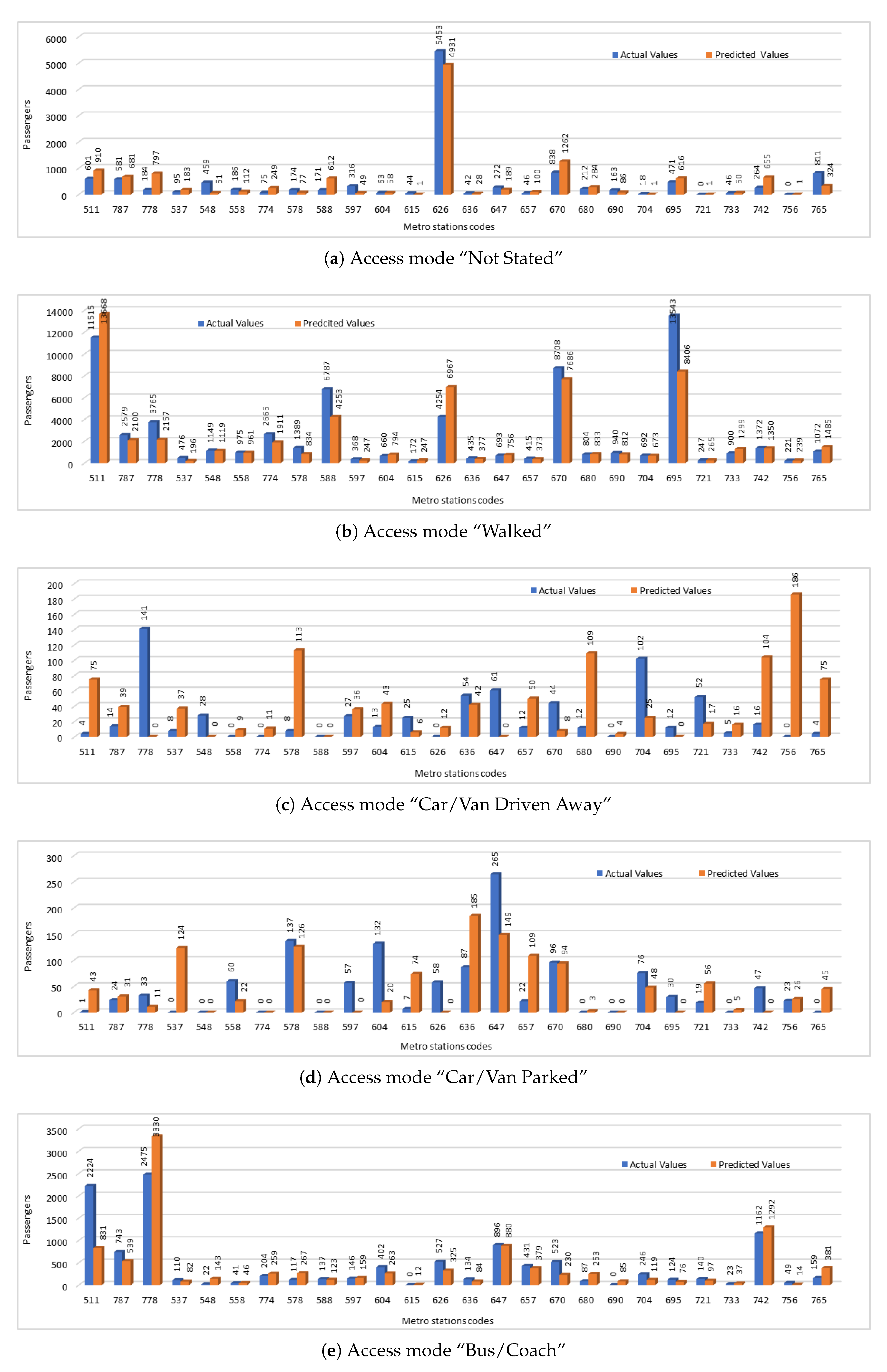
For evaluation of our predicted values, we have compared the predicted values with the actual values. We have presented the predicted passengers values that were entering the stations using five selected access modes including “not stated”, “walked”, “car/van driven away”, “car/van parked”, and “bus/coach”. The comparison of actual number of passengers entering the stations using different access modes and the number of passengers predicted by our deep model is shown in Figure 6. We have used station codes (NLC) in this figure instead of station names. For corresponding station names, please refer to Table 4. Comparison of actual and predicted values shows that in some cases prediction results were close to the actual values and predicted values were showing the same trends even if they were not very close in some cases. In Figure 6a,b,e, we can see where both actual and predicted values are showing the similar trends, but in Figure 6c,d are showing the trends that are not similar. One reason of this error could be the small amount of passenger data which shows the infrequent use of these access modes by the passengers.
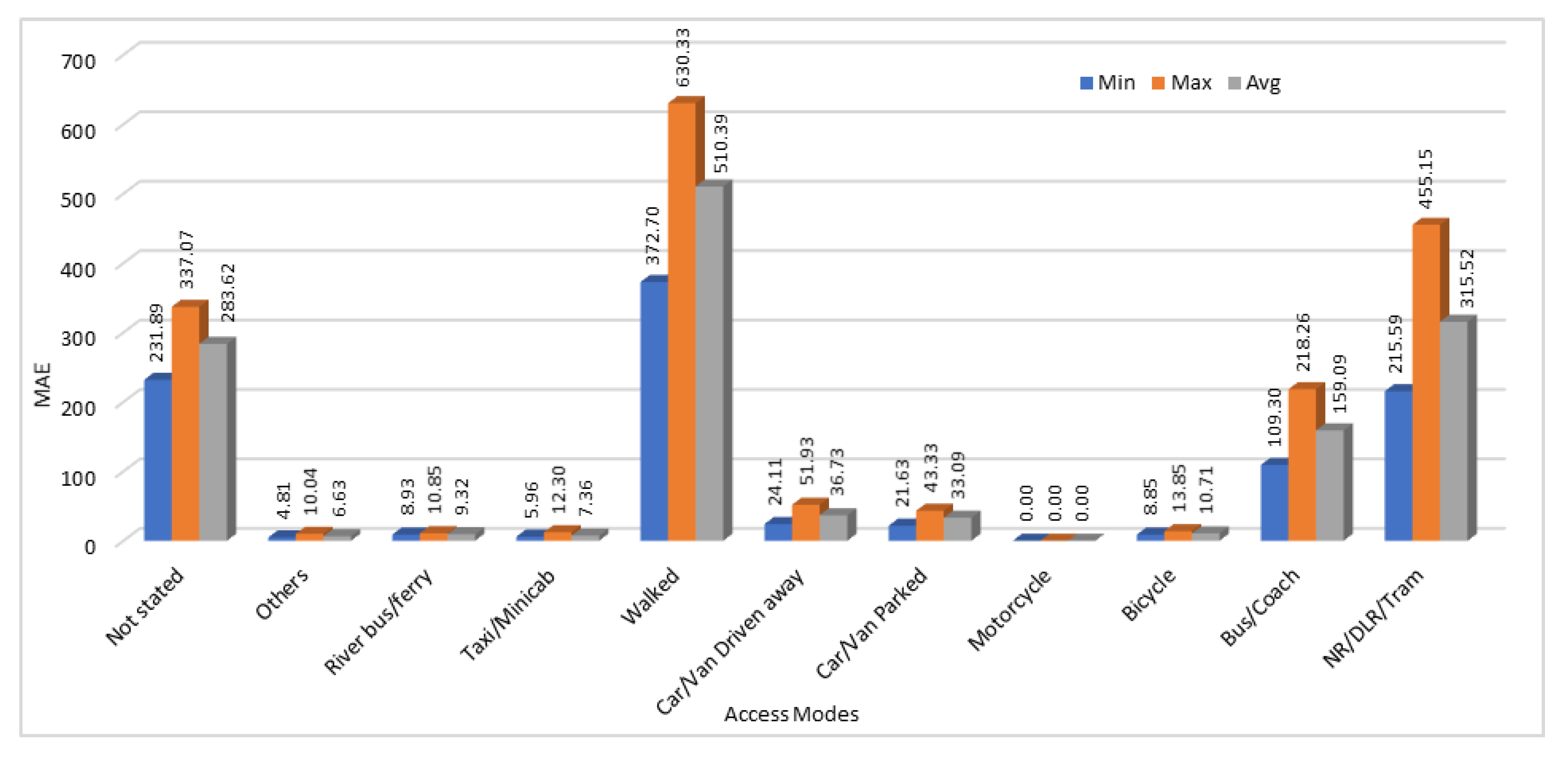
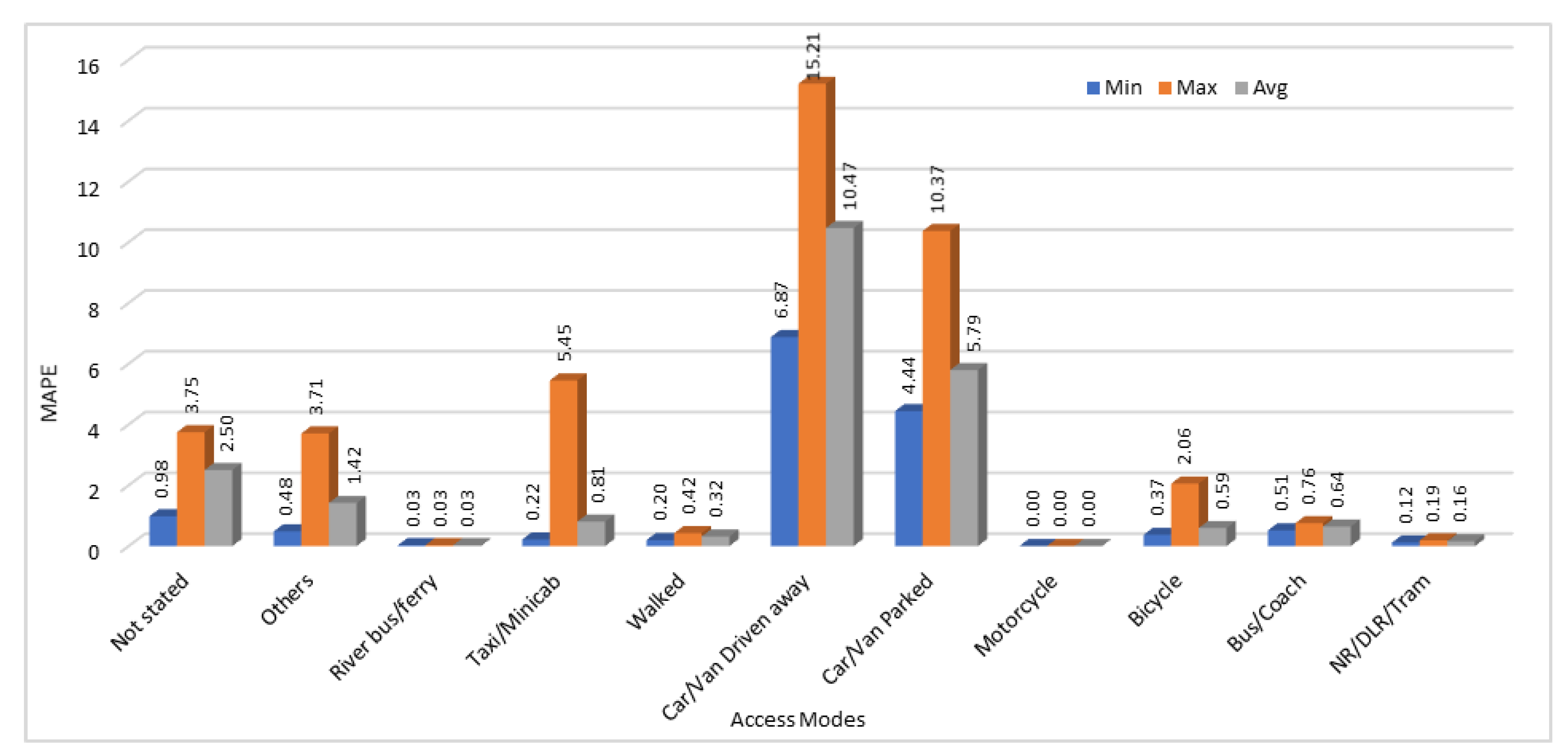
We have calculated MAE, and MAPE for all 25 executions of our model to test the accuracy of predicted results. From those 25 results, we have calculated the minimum errors (MAE and MAPE), maximum error and average error values among 25 generated results. Results obtained by calculating the MAE and MAPE values by comparing the actual and predicted passengers count values are shown in Figure 7 and Figure 8 respectively.
The prediction accuracy shows high variation due to the nature of the dataset. This is clear from the results and by showing minimum, maximum, and average error values for all the access modes. In some cases, there was no change in data across different stations, so the prediction accuracy is very high for those access modes. As shown in Figure 7 and Figure 8, both mean absolute error and mean absolute percentage error values are zero when motorcycle is used as an access mode. This is because the data patterns on all the stations for the number of passengers traveling through motorcycles were same. Therefore, the predicted values for number of passengers using motorcycles to reach the stations were also accurate. In some cases, absolute mean error value was high as compared to other access modes as we can see from Figure 7. We can see that error value for the access mode “walked” is higher than all the other access modes which shows that the predicted values were much different from the actual values. However, if we see the Figure 8, mean absolute percentage error values are very low for those passengers who mentioned the station access mode as “walked”. This is because of a lot of variation in data of passengers who entered the station by walking. In some stations, such passengers were in hundreds, on some stations they were in thousands, and on some stations those were in tens of thousands. Therefore, the MAE is very high because the predicted values are different from the actual values, but the MAPE is comparatively very low that shows that it is tolerable. Same is the case for the access modes “Car/Van driven away” and “Car/Van parked”. In some other cases, such as “Taxi/Minicab”, “River bus/ferry”, “Others”, and "Bicycle”, the error value calculated using MAE was low and it was not very high when using MAPE method as well.

4.2. Predicting Number of Passengers Exiting the Stations using Different Egress Modes

In this section, we have used the dataset that gives the number of passengers exiting the train stations after traveling from their origin stations to the destination stations. The data gives us the number of passengers using different egress modes when exiting the stations to reach their destinations. Same as access modes described above, egress modes have also been divided into different categories based on the nature of transportation means. These include NR/DLR/Tram, Bus/Coach, Bicycle, Motorcycle, Car/Van Parked, Car/Van Driven Away, Walked, Taxi/Minicab, River Bus/Ferry, and Others. In addition to these categories, exiting data collected for passengers who did not describe their means of transportation to reach the station is included by using the tag “Not stated”. This data has also been collected at six different intervals in a day. Same interval names and durations have been used to describe the egress modes as well. To predict the number of passengers using a specific egress mode while leaving the station, we have modeled the relationship between the passengers exiting the stations at different time intervals. We have used the five time intervals (early, am peak, midday, evening, and late) data as input to predict the passengers count at sixth time interval i.e., “p.m. peak”. An overview of the input dataset used in this work is shown in Table 5. This table also shows the egress mode data for selected station (NLC 574) whereas the data for all the other stations is available on the same pattern. Again, we have used 80% data for training purpose, 10% data for testing purpose and the remaining 10% data is used for prediction purposes. For each egress mode, our deep model was executed for 25 times and therefore we collected 25 sets of predicted numbers of passengers for each egress mode.
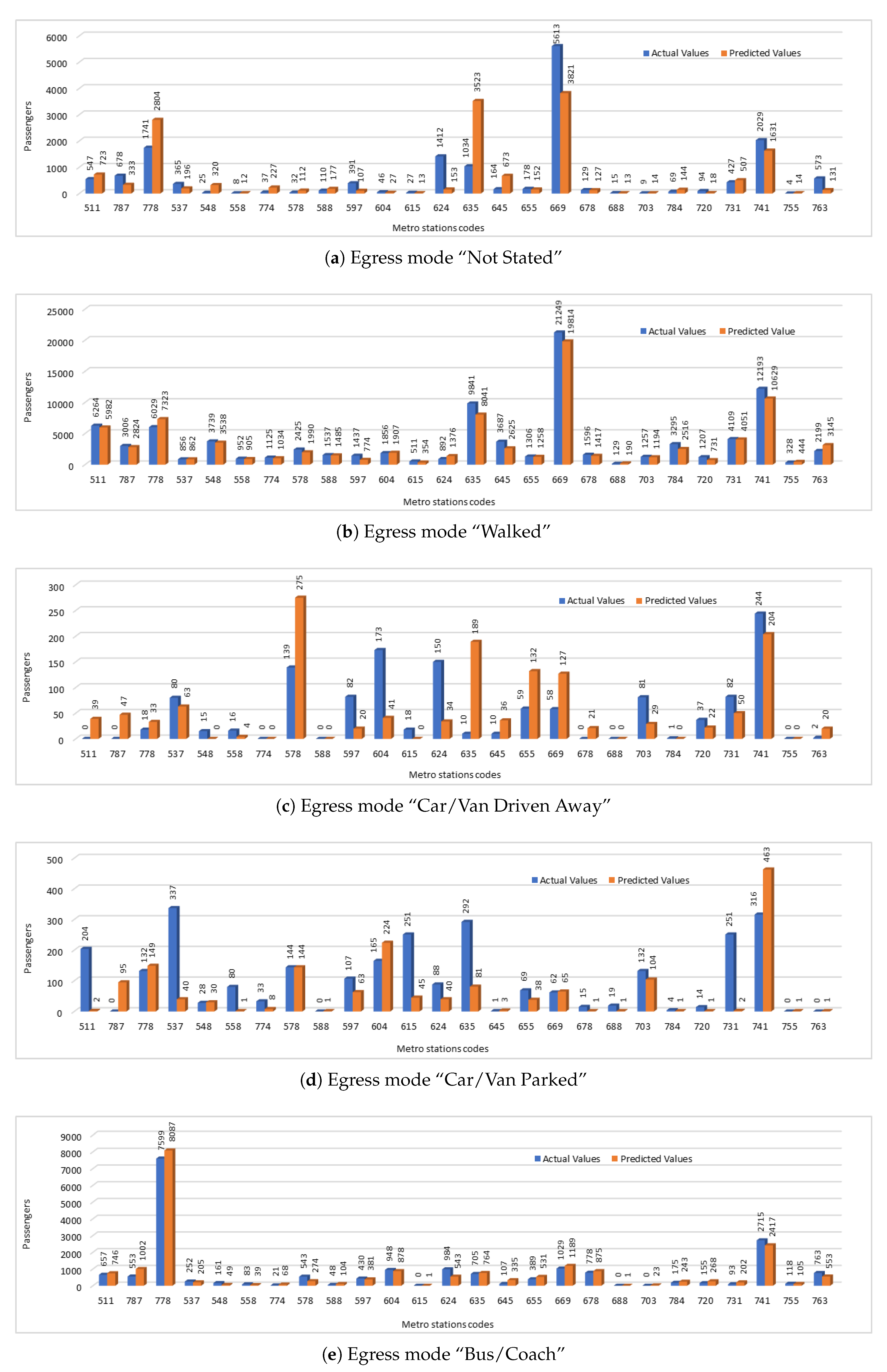
We have compared the original number of passengers exiting the metro stations using selected egress modes with the passengers count predicted by our deep model. Same as we did in access modes, we have 10 different egress modes, but for the comparison of original and predicted values, we have selected five egress modes. The reason to compare the values with only selected egress modes is that some of the modes does not have a reasonable amount of data that could be used to make a meaningful comparison. In Figure 9, we have shown the actual and predicted number of passengers leaving the stations using different egress modes. In these figures, we have used the station codes and number of passengers exiting at different times to predict the number of passengers exiting at “p.m. peak” time interval using different egress modes. To find the station names corresponding to the station codes used in this figure, please see Table 4. If we compare the prediction results, we can say that in some cases, predicted values were very close to the actual values. For example, if we compare the results for egress mode “Walked” Figure 9b, we can see that accuracy is very high in this egress mode. This egress mode also has highest number of passengers reported among other results shown in this figure. Also the predicted number of passengers are very close to the actual number of passengers in case of egress modes “Bus/Coach” Figure 9e. However, if we see the results of “Car/Van Driven Away” or “Car/Van Parked” modes Figure 9c,d we can say that the predicted values are bit different than the actual values and unfortunately the predicted values are not as good as these were in above two cases. One reason of this low accuracy in these two modes could be the high variation in the passenger data. Also, number of passengers in these two cases are very low as compared to the other modes discussed above.
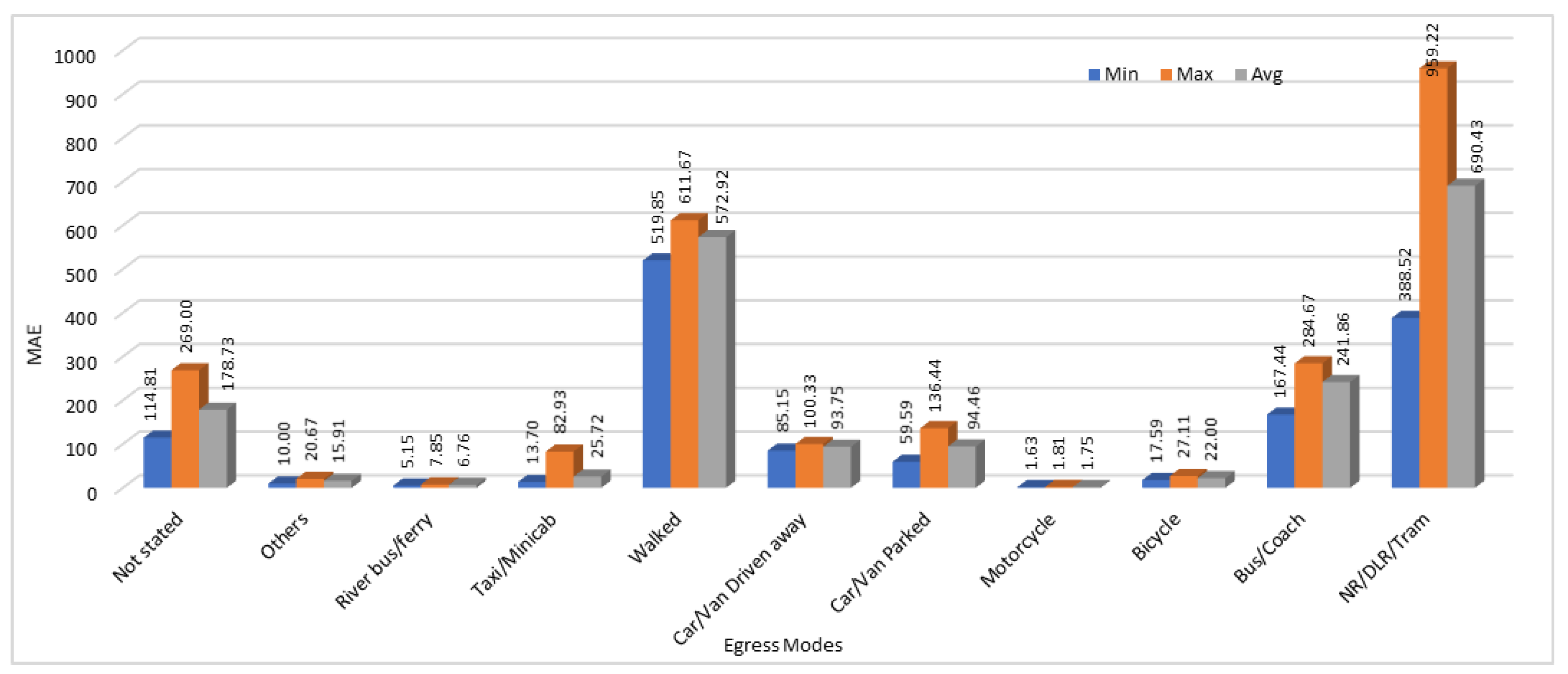
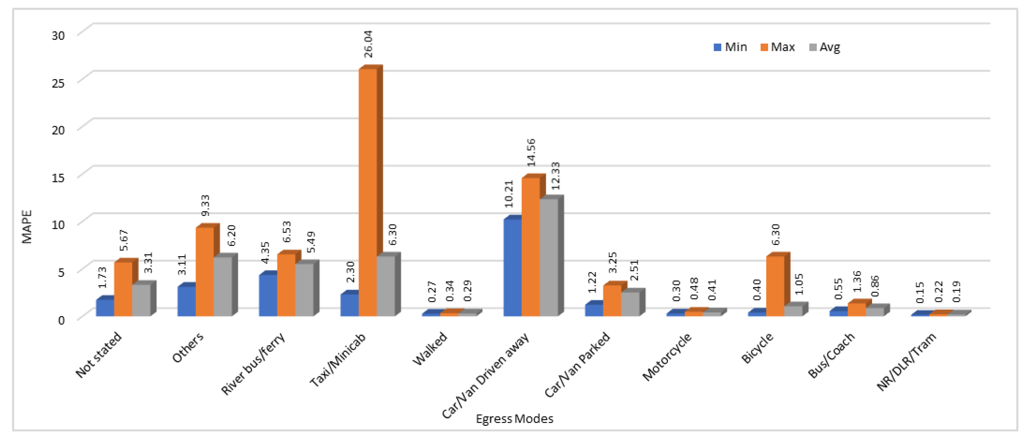
We have calculated the MAE, and MAPE in this section as well to test the accuracy of our model. For evaluation purpose and to compare the results, we have calculated the minimum, maximum, and average error values for all the 25 results obtained by running the same model with same configurations for 10 different egress modes. Minimum, Maximum, and Average MAE and MAPE values calculated by analyzing the all 25 execution results are shown in Figure 10 and Figure 11 respectively.
As we discussed before in access modes, prediction results show high variation in some cases in the egress modes data as well. For egress modes, MAE shows that the two egress modes “walked” and “NR/DLR/Tram” have very high loss values. This is because of the very high values (passengers count) in those two modes. If we see the MAPE calculated for both these modes, it is lowest among all the other egress modes. On the other hand, egress modes “Car/Van driven away” and “river bus/ferry” that show very low loss rate when using MAE, show very high error rate when MAPE is used as a performance metric.

4.3. Passenger Prediction for Specific Time Interval for Origin-Destination Station Pairs

In this section, we have used the dataset that gives the passenger count at different intervals of a day using OD matrix. In this dataset, we are given the number of passengers at six different time intervals (early, am peak, midday, pm peak, evening, and late) in a day. Therefore, OD matrix gives the number of passengers, who traveled from one station to another at different time intervals. There are 267 stations in this dataset and all the trips from one station to others via different routes have been considered in this data.
We have used the same DL model with the same model configurations as we have used before in the previous sections. Here the division of the dataset to be used as training, testing, and prediction has changed. In this case, dataset was divided into the ratio of 60, 30, and 10 percentage for training, testing and prediction, respectively. MAE and MAPE values have been calculated for analysis purpose in this case as well. Also, we are using ReLU as an activation function. The day time has been divided into six time intervals and we are using the number of passengers at five time intervals to predict the number of passengers at sixth time, so number of input features for our DL model is 5 and its output layer produces 1 feature to get a single estimated value. Due to the large amount of data, batch size is now 50 as compared to 5 which we have used previously in other models, but the number of epochs is same i.e., 1000 iterations per model. This model has also been executed 25 times to check the stability of our model and to see the variations.
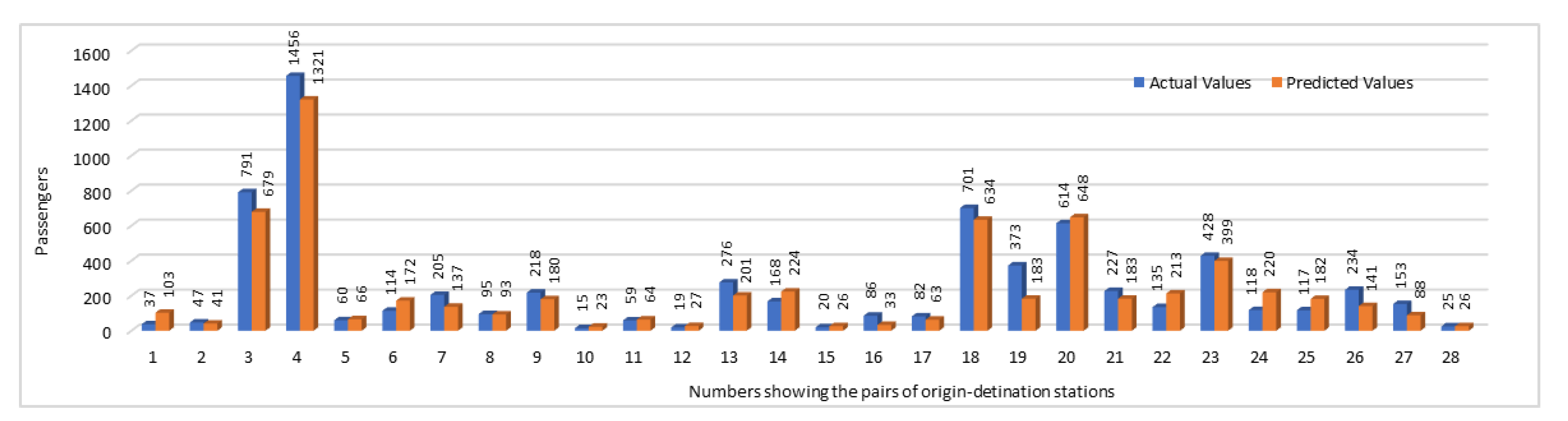
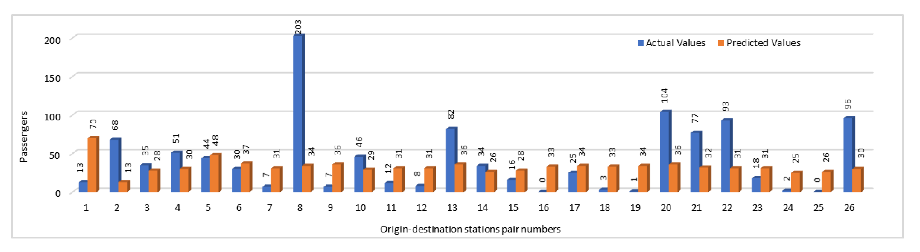
We have compared the predicted numbers of passengers traveling between the OD stations with the original values for selected pairs of OD stations pairs. In this comparison, we have shown the number of passengers traveling between two stations during the time interval “p.m. peak”. Figure 12 gives a comparison of actual and the predicted numbers of passengers. In this figure, instead of using the OD station pairs names, we have used the pairs numbers. To find the corresponding stations pairs names against a pair number shown in the graph, please refer to Table 6. Comparison of actual and predicted values not only provides us the opportunity to analyze the accuracy of prediction results but it also enables us to analyze the OD pairs during that specific time interval based on the number of passengers traveling between them. As far it is concerned to the accuracy of our results, we can see that in most of the stations pairs, predicted values were predicting the accurate trend. Although in some cases, there were some fluctuations in results, but overall, the predicted values have predicted the same trend which was shown by plotting the actual values. This could help the authorities to identify which trains are overloaded with a large number of passengers and which have only a few passengers. They may take the decisions accordingly by reducing number of trips on the routes with less passengers count and can add more trains on the routes where passengers count is high. This way they may generate more revenue as well by saving fuel and other costs on low density routes and by earning more fairs on highly crowded routes.
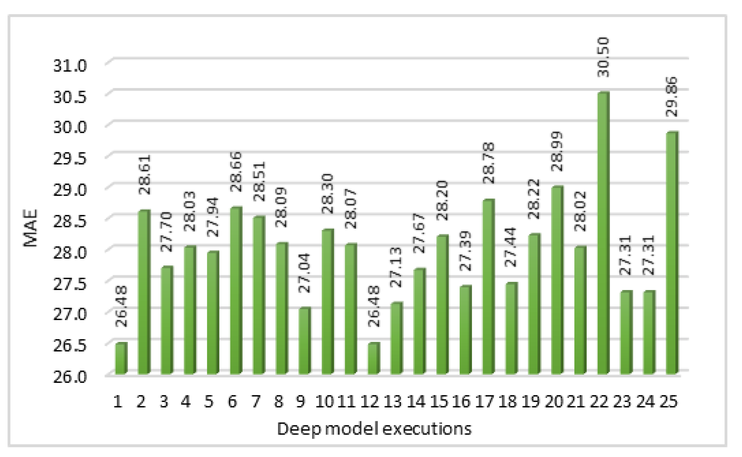
Also, as we are running the same model for 25 times, so we get 25 loss/error values. MAE values calculated by using the prediction values in all 25 executions of our model are shown in the Figure 13. Here, instead of considering the minimum loss value among those results, we are taking the average loss values. We are mainly focusing on the MAE values instead of MAPE values for calculation of error rates. This is due to the reason that our actual data includes zeros as well and MAPE values cannot be calculated if actual value is zero.

4.4. Relationship between the Passenger Count and Distance between the Stations

In this section, we have modeled the relation between the distance between the origin and the destination stations and the number of passengers traveling between these OD pairs. Therefore, we are presenting the results of our deep learning model in which we have used the distance between the train stations and have estimated the number of passengers traveling from one station to another using the OD matrix. Our OD matrix contains the details of more than 34,000 journeys. Around 5 million passengers were surveyed to get the details about their journey on trains from one place/station to other. We have calculated the distance between all the pairs of stations given in the OD matrix and tried to find a relation between the distance between the stations and the number of passengers traveling between those stations at different time intervals in a day. In addition to this, by estimating the number of passengers traveling between any two stations on weekdays, we have tried to investigate if there is any relationship between the distance between the two stations and the number of passengers traveling on a week day. An overview of the dataset used in this section is given in Table 7.
We have predicted the number of passengers traveling between the selected OD stations during the six different time intervals in a day. For this purpose, the deep model was executed with the same configurations set with a batch size of 5 and number of epochs were 1000. In this model, the input data was first changed by considering only the unique origin. The station codes (NLC) for OD stations, and the distance between the OD stations were also used as input parameters while predicting the number of passengers during weekdays. Figure 14 compares the number of passengers traveling between different stations during “weekday”. In this figure, vertical axis shows the number of passengers traveling between the origin and destination stations. Horizontal axis shows the OD pair number as we have not given the names of stations to make it clear on graph. To see the corresponding origin-destination station names against an OD-pair number, please refer to Table 8. In this table, we have given the distance between the ODs stations pairs used in this work to predict the number of passengers traveling between them on weekdays. Comparison of actual and predicted values shows that for small values, the predicted values were close to the actual values but for high data values, it was unable to predict accordingly and there was a big difference between the actual and the predicted values.
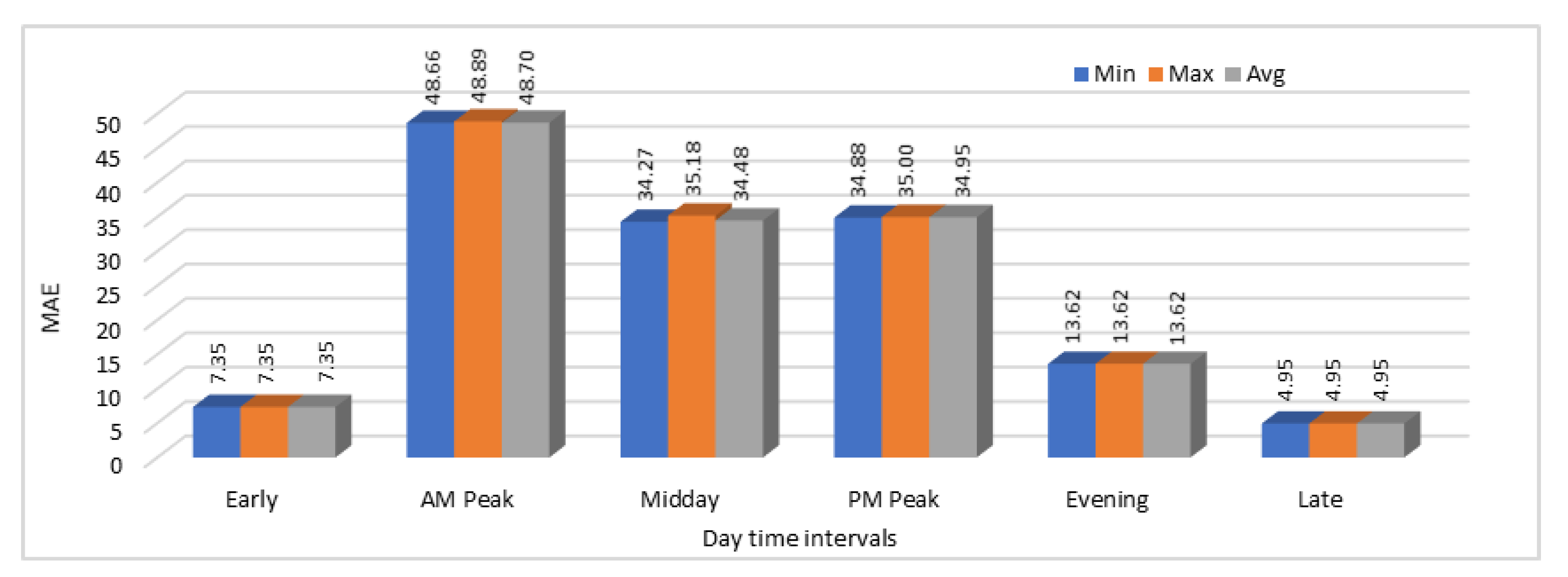
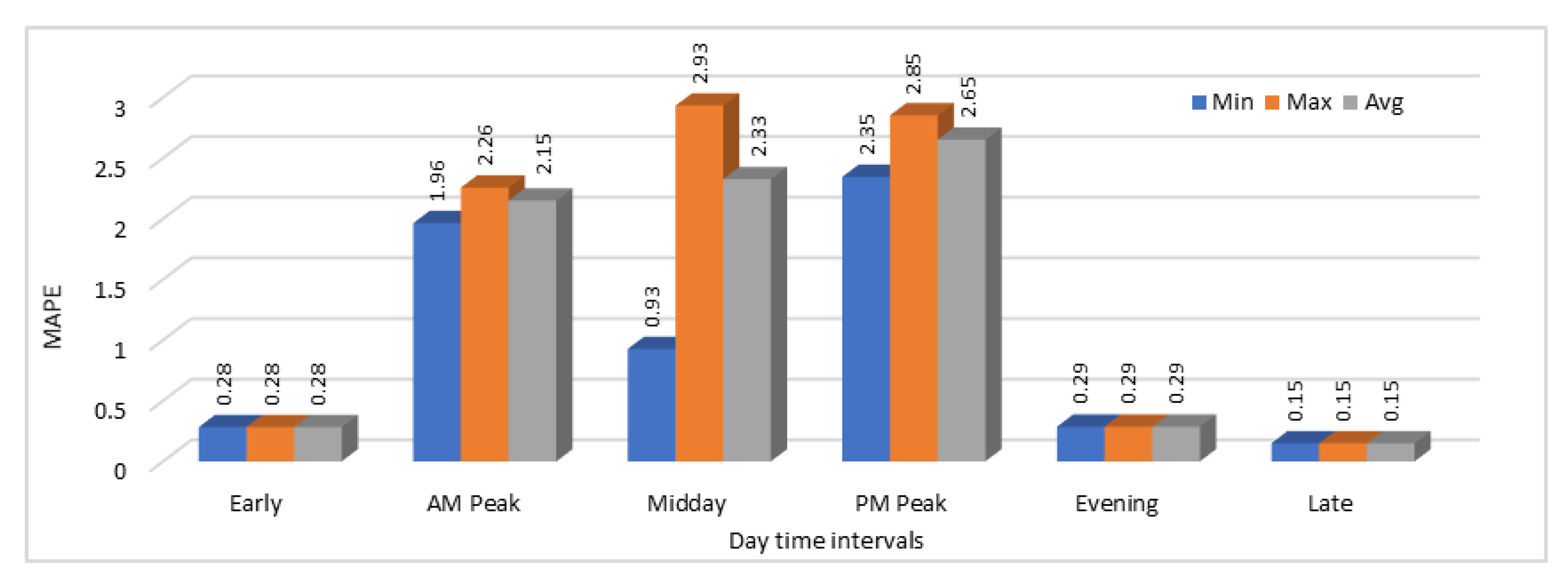
We have calculated both MAE and MAPE values in this case as well and again the model was executed for 25 time with the same configurations and input data to see the variations. MAE and MAPE values obtained by analyzing these results are shown in Figure 15 and Figure 16 respectively. Results show that during some time intervals, error rates were very high as shown for “AM Peak”, “Midday”, and “PM Peak” in Figure 15. Same trend is shown in the MAPE values graph in Figure 16. Another interesting thing about these results is that in all 25 executions of the same model with the same input data, prediction results were almost the same in all the executions because we can see that there are just minor differences in the minimum, maximum, and average MAE and MAPE values.

5. Conclusions and Future Work

Rapid transit systems or metros are a popular choice for high-capacity public transport in urban areas due to their several advantages including safety, dependability, speed, cost, and lower risk of accidents. It is a complex system in itself due to enormous numbers of passengers to be transported through many stations connected through multiple train lines. It becomes even more complex if we are to study and optimize a metro system along with its parent, larger, urban transportation system, including its complementary transportation resources and networks, e.g., trams, buses, ferries, vehicle park and ride stations, motorcycles, bike-sharing stations, and walking routes. This optimization is a gigantic challenge, particularly if we consider complex metro systems in mega-cities, such as the London Metro, the New York City Subway, Tokyo subway system, or the Beijing Subway. Many techniques have been proposed to model, analyze, and design metro systems and these were reviewed in detail in Section 2. However, the current works in this domain have not studied the performance of urban metro systems in sufficiently holistic details. Moreover, existing studies have not adequately benefited from the use of emerging technologies. There is a need for innovative uses of cutting-edge technologies in transportation.
In this paper, we have proposed a comprehensive approach toward large-scale and faster prediction of metro system characteristics by employing the integration of four leading-edge technologies; big data, deep learning, in-memory computing, and GPUs. We have used the London Metro system as a case study to demonstrate the effectiveness of our proposed approach in this paper. We have used the RODS data to predict the number of passengers using different access and egress modes to travel to, and travel from, each of the London Metro stations, respectively. We have also predicted the number of passengers traveling between specific pairs of stations at various time intervals. Moreover, we have predicted the number of passengers traveling between various OD station pairs to investigate the relationship between the number of passengers and the distance between those pairs of stations. The prediction allows better spatiotemporal planning of the whole urban transport system, including the metro subsystem, and its various access and egress modes. We have used CNNs for prediction in our deep learning models. The prediction results were evaluated using MAE and MAPE, and by comparing actual and predicted values of the metro characteristics. A range of prediction accuracies were obtained, from high to fair, and were elaborated on. This is the first study of its kind where integration of leading-edge technologies has been applied to holistic modeling and prediction of a real rapid transit system.
The paper has contributed novel deep learning models, algorithms, implementation, analytics methodology, and software tool for analysis of metro systems. The paper also serves as a preliminary investigation into the convergence of big data and HPC for the transportation sector, specifically for the rapid transit systems, incorporating London Metro as a case study. The convergence has been discussed by researchers in the literature for the last few years (see e.g., [42,43,44,45]). We are not suggesting that this is the first study on the convergence in general, rather it is the first study on the convergence that focuses specifically on the transportation and rapid transit application domains. The topic of HPC and big data convergence is in its infancy and will require many more efforts by the community across diverse applications domains before reaching its maturity. We will explore these convergence issues in the future with the aim to devise novel multidisciplinary technologies for transportation and other sectors.
An important aspect of the work presented in this paper is data analysis and prediction using a distributed computing platform. We have used R [48] and Spark [49] for the purpose. Apache Spark is an improvement over the earlier Hadoop platform. Several other solutions are beginning to emerge for big data during the last few years. These include, among others, Apache Storm [71] and Apache Flink [72]. Apache Storm is a distributed real-time computation platform, particularly well suited toward streaming analytics applications. Apache Flink is another distributed processing engine for stateful computations over data streams [72]. Both these platforms provide myriad of functionalities for distributed processing, particularly for streaming applications. In our case, we are interested in a high-performance, general-purpose, distributed computing platform for both streaming and batch processing of big data. Apache Spark excels in this respect because, compared to both Apache Storm and Apache Flink, it a stable platform with a relatively larger active community of developers. Moreover, Spark is relatively faster, and the development is easier in Spark compared to the other alternatives. Most importantly, Apache Spark is a general-purpose engine and allows integration of a much broader collection of functionalities, tools, and libraries. Future work will investigate the alternatives for the distributed big data computing platforms and consider incorporating cutting-edge technologies for smarter transportation.
Finally, we have integrated multiple technologies to develop in our lab the transportation prediction pipeline proposed in this paper. We manage a supercomputer called Aziz which provides both HPC and big data computational facilities. Aziz was ranked among the Top500 machines in June and November 2015 rankings [73]. We hence have the facilities and motivation to develop in-house complex data processing pipelines. Accessing paid cloud computing resources have also been prohibitive for us due to the costs. This may be different for many researchers due to the lack of facilities and skilled force, and the availability of funds for cloud access. In such cases, or otherwise, similar pipelines can be easily developed and deployed in cloud computing environments. Major cloud vendors such as Amazon and Microsoft are already providing configurable big data analysis pipelines include access to GPUs and in-memory computing platforms. It is foreseen that ICT solutions will increasingly be delivered using the cloud, fog, and edge computing paradigms. We aim to do the same; i.e., to deliver the rapid transit software using cloud computing. This would form another topic for our future research.

Author Contributions

Conceptualization, M.A. and R.M.; methodology, M.A. and R.M.; software, M.A.; validation, M.A. and R.M.; formal analysis, M.A. and R.M.; investigation, M.A. and R.M.; resources, R.M., I.K., A.A. (Ahmed Alzahrani), A.A. (Aiiad Albeshri) and S.M.A.; data curation, M.A.; writing—original draft preparation, M.A. and R.M.; writing—review and editing, R.M.; visualization, M.A. and R.M.; supervision, R.M.; project administration, R.M. and A.A. (Aiiad Albeshri); funding acquisition, R.M., A.A. (Ahmed Alzahrani), A.A. (Aiiad Albeshri), I.K. and S.M.A.

Funding

This project was funded by the Deanship of Scientific Research (DSR) at King Abdulaziz University, Jeddah, under grant number RG-11-611-40. The authors, therefore, acknowledge with thanks DSR for technical and financial support.

Acknowledgments

The experiments performed in this paper were executed on the Aziz supercomputer being managed by the HPC Center at the King Abdulaziz University. We are thankful to the anonymous editor and reviewers whose recommendations have helped us greatly to improve this paper.

Conflicts of Interest

The authors declare no conflict of interest. The funders had no role in the design of the study; in the collection, analyses, or interpretation of data; in the writing of the manuscript, or in the decision to publish the results.

References

  1. World Health Organization. Road Traffic Injuries. 2018. Available online: http://www.who.int/news-room/fact-sheets/detail/road-traffic-injuries (accessed on 27 November 2018).
  2. El Hatri, C.; Boumhidi, J. Traffic management model for vehicle re-routing and traffic light control based on Multi-Objective Particle Swarm Optimization. Intell. Decis. Technol. 2017, 11, 199–208. [Google Scholar] [CrossRef]
  3. Hu, Z.; Yan, Y.; Qiu, Z. Research on Optimization Model of Making Inter-city Passenger Train Operation Plan and Ticket Price. In Proceedings of the International Conference on Information Management, Innovation Management and Industrial Engineering (ICIII’08), Taipei, Taiwan, 19–21 December 2008; Volume 3, pp. 45–48. [Google Scholar]
  4. Sun, X.; Zhang, S.; Dong, H.; Zhu, H. Optimal train schedule with headway and passenger flow dynamic models. In Proceedings of the 2013 IEEE International Conference on Intelligent Rail Transportation (ICIRT), Beijing, China, 30 August–1 September 2013; pp. 307–312. [Google Scholar]
  5. Escolano, C.O.; Dadios, E.P.; Fillone, A.D. A neural network model of optimal scheduling system of public utility buses in Epifanio Delos Santos Avenue (EDSA). In Proceedings of the 2015 International Conference on Humanoid, Nanotechnology, Information Technology, Communication and Control, Environment and Management (HNICEM), Cebu City, Philippines, 9–12 December 2015; pp. 1–5. [Google Scholar]
  6. Wang, R.; Work, D.B. Data driven approaches for passenger train delay estimation. In Proceedings of the 2015 IEEE 18th International Conference on Intelligent Transportation Systems (ITSC), Las Palmas, Spain, 15–18 May 2015; pp. 535–540. [Google Scholar]
  7. Wang, P.; Wu, C.; Gao, X. Research on subway passenger flow combination prediction model based on RBF neural networks and LSSVM. In Proceedings of the 2016 Chinese Control and Decision Conference (CCDC), Yinchuan, China, 28–30 May 2016; pp. 6064–6068. [Google Scholar]
  8. Abadi, A.M.; Wutsqa, D.U. Neuro fuzzy model with singular value decomposition for forecasting the number of train passengers in Yogyakarta. In Proceedings of the 2014 11th International Conference on Fuzzy Systems and Knowledge Discovery (FSKD), Xiamen, China, 19–21 August 2014; pp. 178–182. [Google Scholar]
  9. Zhang, P.; Liu, X.; Chen, M. Optimal train scheduling under a flexible skip-stop scheme for urban rail transit based on smartcard data. In Proceedings of the 2016 IEEE International Conference on Intelligent Rail Transportation (ICIRT), Birmingham, UK, 23–25 August 2016; pp. 13–22. [Google Scholar]
  10. Zhao, J.; Zhang, F.; Tu, L.; Xu, C.; Shen, D.; Tian, C.; Li, X.Y.; Li, Z. Estimation of passenger route choice pattern using smart card data for complex metro systems. IEEE Trans. Intell. Transp. Syst. 2017, 18, 790–801. [Google Scholar] [CrossRef]
  11. Mehmood, R.; See, S.; Katib, I.; Chlamtac, I. (Eds.) Smart Infrastructure and Applications: Foundations for Smarter Cities and Societies; EAI/Springer Innovations in Communication and Computing; Springer International Publishing: Cham, Switzerland, 2019; p. 692. [Google Scholar] [CrossRef]
  12. Mehmood, R.; Bhaduri, B.; Katib, I.; Chlamtac, I. (Eds.) Smart Societies, Infrastructure, Technologies and Applications; Lecture Notes of the Institute for Computer Sciences, Social Informatics and Telecommunications Engineering (LNICST); Springer International Publishing: Cham, Switzerland, 2018; Volume 224. [Google Scholar]
  13. Mehmood, R.; Alam, F.; Albogami, N.N.; Katib, I.; Albeshri, A.; Altowaijri, S.M. UTiLearn: A personalised ubiquitous teaching and learning system for smart societies. IEEE Access 2017, 5, 2615–2635. [Google Scholar] [CrossRef]
  14. Muhammed, T.; Mehmood, R.; Albeshri, A.; Katib, I. UbeHealth: A Personalized Ubiquitous Cloud and Edge-Enabled Networked Healthcare System for Smart Cities. IEEE Access 2018, 6, 32258–32285. [Google Scholar] [CrossRef]
  15. Büscher, M.; Coulton, P.; Efstratiou, C.; Gellersen, H.; Hemment, D.; Mehmood, R.; Sangiorgi, D. Intelligent mobility systems: some socio-technical challenges and opportunities. In International Conference on Communications Infrastructure. Systems and Applications in Europe; Springer: Berlin/Heidelberg, Germany, 2009; pp. 140–152. [Google Scholar]
  16. Arfat, Y.; Aqib, M.; Mehmood, R.; Albeshri, A.; Katib, I.; Albogami, N.; Alzahrani, A. Enabling Smarter Societies through Mobile Big Data Fogs and Clouds. Procedia Comput. Sci. 2017, 109, 1128–1133. [Google Scholar] [CrossRef]
  17. Mehmood, R.; Graham, G. Big data logistics: A health-care transport capacity sharing model. Procedia Comput. Sci. 2015, 64, 1107–1114. [Google Scholar] [CrossRef]
  18. Arfat, Y.; Mehmood, R.; Albeshri, A. Parallel Shortest Path Graph Computations of United States Road Network Data on Apache Spark. In International Conference on Smart Cities, Infrastructure, Technologies and Applications; Springer International Publishing: Cham, Switzerland, 2017; pp. 323–336. [Google Scholar]
  19. Mehmood, R.; Meriton, R.; Graham, G.; Hennelly, P.; Kumar, M. Exploring the influence of big data on city transport operations: a Markovian approach. Int. J. Oper. Prod. Manag. 2017, 37, 75–104. [Google Scholar] [CrossRef] [Green Version]
  20. Mehmood, R.; Faisal, M.A.; Altowaijri, S. Future Networked Healthcare Systems: A Review and Case Study. In Handbook of Research on Redesigning the Future of Internet Architectures; Boucadair, M., Jacquenet, C., Eds.; IGI Global: Hershey, PA, USA, 2015; pp. 531–558. [Google Scholar]
  21. Mehmood, R.; Lu, J.A. Computational Markovian analysis of large systems. J. Manuf. Technol. Manag. 2011, 22, 804–817. [Google Scholar] [CrossRef]
  22. Aqib, M.; Mehmood, R.; Albeshri, A.; Alzahrani, A. Disaster Management in Smart Cities by Forecasting Traffic Plan Using Deep Learning and GPUs. In International Conference on Smart Cities, Infrastructure, Technologies and Applications (SCITA 2017): Smart Societies, Infrastructure, Technologies and Applications; Mehmood, R., Bhaduri, B., Katib, I., Chlamtac, I., Eds.; Springer International Publishing: Cham, Switzerland, 2018; pp. 139–154. [Google Scholar]
  23. Alazawi, Z.; Altowaijri, S.; Mehmood, R.; Abdljabar, M.B. Intelligent disaster management system based on cloud-enabled vehicular networks. In Proceedings of the IEEE 2011 11th International Conference on ITS Telecommunications (ITST), St. Petersburg, Russia, 23–25 August 2011; pp. 361–368. [Google Scholar]
  24. Alazawi, Z.; Abdljabar, M.B.; Altowaijri, S.; Vegni, A.M.; Mehmood, R. ICDMS: an intelligent cloud based disaster management system for vehicular networks. In International Workshop on Communication Technologies for Vehicles, Proceedings of the Nets4Cars/Nets4Trains 2012, Vilnius, Lithuania, 25–27 April 2012; Lecture Notes in Computer Science Book Series (LNCS); Springer: Berlin/Heidelberg, Germany, 2012; Volume 7266, pp. 40–56. [Google Scholar]
  25. Alazawi, Z.; Alani, O.; Abdljabar, M.B.; Altowaijri, S.; Mehmood, R. A smart disaster management system for future cities. In Proceedings of the 2014 ACM International Workshop on Wireless and Mobile Technologies for Smart Cities, Philadelphia, PA, USA, 11 August 2014; ACM: New York, NY, USA, 2014; pp. 1–10. [Google Scholar]
  26. Alazawi, Z.; Alani, O.; Abdljabar, M.B.; Mehmood, R. An intelligent disaster management system based evacuation strategies. In Proceedings of the 2014 9th International Symposium onCommunication Systems, Networks & Digital Signal Processing (CSNDSP), Manchester, UK, 23–25 July 2014; pp. 673–678. [Google Scholar]
  27. Alam, F.; Mehmood, R.; Katib, I. D2TFRS: An object recognition method for autonomous vehicles based on RGB and spatial values of pixels. In Lecture Notes of the Institute for Computer Sciences, Social-Informatics and Telecommunications Engineering; Springer: Cham, Switzerland, 2018; Volume 224, pp. 155–168. [Google Scholar]
  28. Aqib, M.; Mehmood, R.; Alzahrani, A.; Katib, I. A Smart Disaster Management System for Future Cities using Deep Learning, GPUs, and In-Memory Computing. In Smart Infrastructure and Applications: Foundations for Smarter Cities and Societies; Mehmood, R., See, S., Katib, I., Chlamtac, I., Eds.; Springer International Publishing: Cham, Switzerland, 2019. [Google Scholar]
  29. Aqib, M.; Mehmood, R.; Alzahrani, A.; Katib, I. In-Memory Deep Learning Computations on GPUs for Prediction of Road Traffic Incidents Using Big Data Fusion. In Smart Infrastructure and Applications: Foundations for Smarter Cities and Societies; Mehmood, R., See, S., Katib, I., Chlamtac, I., Eds.; Springer International Publishing: Cham, Switzerland, 2019. [Google Scholar]
  30. Aqib, M.; Mehmood, R.; Alzahrani, A.; Katib, I.; Albeshri, A. A Deep Learning Model to Predict Vehicles Occupancy on Freeways for Traffic Management. Int. J. Comput. Sci. Netw. Secur. 2018, 18, 246–254. [Google Scholar]
  31. Graham, G.; Mehmood, R.; Coles, E. Exploring future cityscapes through urban logistics prototyping: A technical viewpoint. Supply Chain Manag. 2015, 20, 341–352. [Google Scholar] [CrossRef]
  32. Mehmood, R.; Nekovee, M. Vehicular ad hoc and grid networks: Discussion, design and evaluation. In Proceedings of the 14th World Congress On Intelligent Transport Systems (ITS), Beijing, China, 9–13 October 2007. [Google Scholar]
  33. Gillani, S.; Shahzad, F.; Qayyum, A.; Mehmood, R. A survey on security in vehicular ad hoc networks. In Proceedings of the International Workshop on Communication Technologies for Vehicles, Villeneuve d’ Ascq, France, 14–15 May 2013; Lecture Notes in Computer Science. Springer: Berlin/Heidelberg, Germany, 2013; Volume 7865, pp. 59–74. [Google Scholar]
  34. Alvi, A.; Greaves, D.; Mehmood, R. Intra-vehicular verification and control: A two-pronged approach. In Proceedings of the 2010 7th International Symposium on Communication Systems, Networks & Digital Signal Processing (CSNDSP 2010), Newcastle upon Tyne, UK, 21–23 July 2013; pp. 401–405. [Google Scholar]
  35. Nabi, Z.; Alvi, A.; Mehmood, R. Towards standardization of in-car sensors. In International Workshop on Communication Technologies for Vehicles; Springer International Publishing: Cham, Switzerland, 2011; pp. 216–223. [Google Scholar]
  36. Schlingensiepen, J.; Mehmood, R.; Nemtanu, F.C.; Niculescu, M. Increasing sustainability of road transport in European cities and metropolitan areas by facilitating autonomic road transport systems (ARTS). In Sustainable Automotive Technologies 2013; Springer International Publishing: Cham, Switzerland, 2014; pp. 201–210. [Google Scholar]
  37. Schlingensiepen, J.; Nemtanu, F.; Mehmood, R.; McCluskey, L. Autonomic transport management systems-enabler for smart cities, personalized medicine, participation and industry grid/industry 4.0. In Intelligent Transportation Systems—Problems and Perspectives; Springer International Publishing: Cham, Switzerland, 2016; pp. 3–35. [Google Scholar]
  38. Schlingensiepen, J.; Mehmood, R.; Nemtanu, F.C. Framework for an autonomic transport system in smart cities. Cybern. Inf. Technol. 2015, 15, 50–62. [Google Scholar] [CrossRef]
  39. Suma, S.; Mehmood, R.; Albugami, N.; Katib, I.; Albeshri, A. Enabling Next Generation Logistics and Planning for Smarter Societies. Procedia Comput. Sci. 2017, 109, 1122–1127. [Google Scholar] [CrossRef]
  40. Suma, S.; Mehmood, R.; Albeshri, A. Automatic Event Detection in Smart Cities Using Big Data Analytics. In International Conference on Smart Cities, Infrastructure, Technologies and Applications; Springer International Publishing: Cham, Switzerland, 2017; pp. 111–122. [Google Scholar]
  41. Alomari, E.; Mehmood, R. Analysis of tweets in Arabic language for detection of road traffic conditions. In Lecture Notes of the Institute for Computer Sciences, Social-Informatics and Telecommunications Engineering; Springer: Cham, Switzerland, 2018; Volume 224, pp. 98–110. [Google Scholar]
  42. Reed, D.A.; Dongarra, J. Exascale Computing and Big Data. Commun. ACM 2015, 58, 56–68. [Google Scholar] [CrossRef]
  43. Fox, G.; Qiu, J.; Jha, S.; Ekanayake, S.; Kamburugamuve, S. Big Data, Simulations and HPC Convergence. In Big Data Benchmarking, WBDB 2015; Rabl, T., Nambiar, R., Baru, C., Bhandarkar, M., Poess, M., Pyne, S., Eds.; Lecture Notes in Computer Science (LNCS); Springer: Cham, Switzerland, 2016; Volume 10044, pp. 3–17. [Google Scholar]
  44. Farber, R. The Convergence of Big Data and Extreme-Scale HPC; HPCWire: San Diego, CA, USA, 2018. [Google Scholar]
  45. Usman, S.; Mehmood, R.; Katib, I. Big data and HPC convergence: The cutting edge and outlook. In International Conference on Smart Cities, Infrastructure, Technologies and Applications (SCITA 2017); Lecture Notes of the Institute for Computer Sciences, Social-Informatics and Telecommunications Engineering; Springer: Cham, Switzerland, 2018; Volume 224, pp. 11–26. [Google Scholar]
  46. Transport for London. London Underground. 2018. Available online: https://tfl.gov.uk/corporate/about-tfl/what-we-do/london-underground (accessed on 25 October 2018).
  47. Transport for London. TfL Rolling Origin and Destination Survey. 2015. Available online: https://data.london.gov.uk/dataset/tfl-rolling-origin-and-destination-survey (accessed on 25 October 2018).
  48. R Core Team. R: A Language and Environment for Statistical Computing; R Foundation for Statistical Computing: Vienna, Austria, 2013. [Google Scholar]
  49. Zaharia, M.; Xin, R.S.; Wendell, P.; Das, T.; Armbrust, M.; Dave, A.; Meng, X.; Rosen, J.; Venkataraman, S.; Franklin, M.J.; et al. Apache spark: A unified engine for big data processing. Commun. ACM 2016, 59, 56–65. [Google Scholar] [CrossRef]
  50. Lianbo, D. Optimal model and algorithm of passenger train plan. In Proceedings of the IEEE 27th Chinese Control Conference (CCC 2008), Kunming, China, 16–18 July 2008; pp. 613–616. [Google Scholar]
  51. Li, S.; De Schutter, B.; Yang, L.; Gao, Z. Robust model predictive control for train regulation in underground railway transportation. IEEE Trans. Control Syst. Technol. 2016, 24, 1075–1083. [Google Scholar] [CrossRef]
  52. Jiang, Z.; Hsu, C.H.; Zhang, D.; Zou, X. Evaluating rail transit timetable using big passengers’ data. J. Comput. Syst. Sci. 2016, 82, 144–155. [Google Scholar] [CrossRef]
  53. Poonawala, H.; Kolar, V.; Blandin, S.; Wynter, L.; Sahu, S. Singapore in motion: Insights on public transport service level through farecard and mobile data analytics. In Proceedings of the 22nd ACM SIGKDD International Conference on Knowledge Discovery and Data Mining, San Francisco, CA, USA, 13–17 August 2016; ACM: New York, NY, USA, 2016; pp. 589–598. [Google Scholar]
  54. Xu, X.; Li, K.; Yang, L. Scheduling heterogeneous train traffic on double tracks with efficient dispatching rules. Transp. Res. Part B Methodol. 2015, 78, 364–384. [Google Scholar] [CrossRef]
  55. Li, S.; Yang, L.; Gao, Z.; Li, K. Robust train regulation for metro lines with stochastic passenger arrival flow. Inf. Sci. 2016, 373, 287–307. [Google Scholar] [CrossRef]
  56. Yue, Y.; Wang, S.; Zhou, L.; Tong, L.; Saat, M.R. Optimizing train stopping patterns and schedules for high-speed passenger rail corridors. Transp. Res. Part C Emerg. Technol. 2016, 63, 126–146. [Google Scholar] [CrossRef]
  57. Yang, L.; Qi, J.; Li, S.; Gao, Y. Collaborative optimization for train scheduling and train stop planning on high-speed railways. Omega 2016, 64, 57–76. [Google Scholar] [CrossRef]
  58. Samà, M.; Corman, F.; Pacciarelli, D. A variable neighbourhood search for fast train scheduling and routing during disturbed railway traffic situations. Comput. Oper. Res. 2017, 78, 480–499. [Google Scholar]
  59. Yin, J.; Yang, L.; Tang, T.; Gao, Z.; Ran, B. Dynamic passenger demand oriented metro train scheduling with energy-efficiency and waiting time minimization: Mixed-integer linear programming approaches. Transp. Res. Part B Methodol. 2017, 97, 182–213. [Google Scholar] [CrossRef]
  60. Sinha, S.K.; Salsingikar, S.; SenGupta, S. An iterative bi-level hierarchical approach for train scheduling. J. Rail Transp. Plan. Manag. 2016, 6, 183–199. [Google Scholar] [CrossRef]
  61. Corman, F.; D’Ariano, A.; Marra, A.D.; Pacciarelli, D.; Samà, M. Integrating train scheduling and delay management in real-time railway traffic control. Transp. Res. Part E Logist. Transp. Rev. 2017, 105, 213–239. [Google Scholar] [CrossRef]
  62. Shiwakoti, N.; Tay, R.; Stasinopoulos, P.; Woolley, P.J. Likely behaviours of passengers under emergency evacuation in train station. Saf. Sci. 2017, 91, 40–48. [Google Scholar] [CrossRef]
  63. He, Y.; Blandin, S.; Wynter, L.; Trager, B. Analysis and real-time prediction of local incident impact on transportation networks. In Proceedings of the 2014 IEEE International Conference on Data Mining Workshop (ICDMW), Shenzhen, China, 14 December 2014; pp. 158–166. [Google Scholar]
  64. Pan, B.; Demiryurek, U.; Shahabi, C.; Gupta, C. Forecasting spatiotemporal impact of traffic incidents on road networks. In Proceedings of the 2013 IEEE 13th International Conference on Data Mining (ICDM), Dallas, TX, USA, 7–10 December 2013; pp. 587–596. [Google Scholar]
  65. Miller, M.; Gupta, C. Mining traffic incidents to forecast impact. In Proceedings of the ACM SIGKDD International Workshop on Urban Computing, Beijing, China, 12 August 2012; ACM: New York, NY, USA, 2012; pp. 33–40. [Google Scholar]
  66. Chung, Y.; Recker, W.W. A methodological approach for estimating temporal and spatial extent of delays caused by freeway accidents. IEEE Trans. Intell. Transp. Syst. 2012, 13, 1454–1461. [Google Scholar] [CrossRef]
  67. Pan, B.; Demiryurek, U.; Shahabi, C. Utilizing real-world transportation data for accurate traffic prediction. In Proceedings of the 2012 IEEE 12th International Conference on Data Mining (ICDM), Brussels, Belgium, 10–13 December 2012; pp. 595–604. [Google Scholar]
  68. Ma, X.; Yu, H.; Wang, Y.; Wang, Y. Large-scale transportation network congestion evolution prediction using deep learning theory. PLoS ONE 2015, 10, e0119044. [Google Scholar] [CrossRef]
  69. Abadi, M.; Agarwal, A.; Barham, P.; Brevdo, E.; Chen, Z.; Citro, C.; Corrado, G.S.; Davis, A.; Dean, J.; Devin, M.; et al. TensorFlow: Large-Scale Machine Learning on Heterogeneous Systems. 2015. Available online: https://www.tensorflow.org (accessed on 1 April 2019).
  70. Chollet, F. Keras. 2015. Available online: https://keras.io (accessed on 1 April 2019).
  71. Apache Storm. Available online: https://storm.apache.org/ (accessed on 3 May 2018).
  72. Apache Flink. Available online: https://flink.apache.org/ (accessed on 3 May 2018).
  73. Top500. The Aziz Supercomputer. 2015. Available online: https://www.top500.org/site/50585 (accessed on 3 May 2018).
Figure 1. A Map of the London Metro Network (Courtesy: http://taxomita.com).
Sustainability 11 02736 g001
Figure 2. The Proposed Method for the Integration of Four Technologies.
Sustainability 11 02736 g002
Figure 3. The Process Flow Diagram of the Proposed Method.
Sustainability 11 02736 g003
Figure 4. RODS Dataset: Samples of Data.
Sustainability 11 02736 g004
Figure 5. Deep Learning Model Architecture: one Input, one Output, Three Hidden Layers.
Sustainability 11 02736 g005
Figure 6. Comparison of Actual and Predicted Values: Access Modes (Section 4.1).
Sustainability 11 02736 g006
Figure 7. Minimum, Maximum, and Average MAE Values: Prediction of Access Modes (Section 4.1).
Sustainability 11 02736 g007
Figure 8. Minimum, Maximum, and Average MAPE Values: Access Modes (Section 4.1).
Sustainability 11 02736 g008
Figure 9. Comparison of Actual and Predicted Values: Egress Modes (Section 4.2).
Sustainability 11 02736 g009
Figure 10. Minimum, Maximum, and Average MAE Values: Prediction of Egress Modes (Section 4.2).
Sustainability 11 02736 g010
Figure 11. Minimum, Maximum, and Average MAPE Values: Prediction of Egress Modes (Section 4.2).
Sustainability 11 02736 g011
Figure 12. Comparison of Actual and Predicted Values: Number of Passengers Traveling between OD Station Pairs during the Time Interval “PM Peak” (Section 4.3).
Sustainability 11 02736 g012
Figure 13. MAE Values: Predicting the Number of Passengers using OD Matrix data input (Section 4.3).
Sustainability 11 02736 g013
Figure 14. Passengers traveling between two stations during “weekday” (Section 4.4).
Sustainability 11 02736 g014
Figure 15. Minimum, maximum, and average MAE values when predicting passengers considering the distance between stations (Section 4.4).
Sustainability 11 02736 g015
Figure 16. Minimum, maximum, and average MAPE values when predicting passengers considering the distance between stations (Section 4.4).
Sustainability 11 02736 g016
Table 1. Dataset: Access and Egress Modes.
Sr.NoAttribute NameDescription
1NLCNational location code, it is a code assigned to each station and ticket issuing point in UK.
2Station nameName of the train station where the data has been collected.
3Time periodTime interval for which data has been collected for different access/egress modes. Time interval values include early, am peak, midday, pm peak, evening, late, and total day.
4NR/DLR/TramNumber of passengers used this access/mode while entering/exiting the station.
5Bus/CoachNumber of passengers entered/exited the stations using bus or coach.
6BicycleNumber of passengers who used bicycle to reach station or back to home.
7MotorcycleNumber of passengers who used motorcycle as their access/egress mode.
8Car/Van ParkedPassengers who reached the station by their own car/van and parked it to be used while exiting the station.
9Car/Van Driven AwayNumber of passengers who entered/exited the station by car/van not parked at station.
10WalkedPassengers who did not used any means of transportation to enter/exit the station.
11Taxi/MinicabNumber of passengers who used taxi or minicab as their access/egress mode.
12River Bus/FerryPassengers who used this access/egress mode.
13OtherNumber of passengers who used any other mode of transportation are put in this category.
14Not StatedNumber of passengers who did not describe their access/egress mode are given in this category.
15Total all modesTotal number of passengers entering/exiting the station irrespective of their access/egress modes are given.
Table 2. Dataset: Key Terms used in Prediction of Passengers based on Origin-Destination Station Pairs.
Sr.NoAttribute NameDescription
1FromGives both NLC and station name where the passenger stated his journey.
2ToNLC and the station name of the destination metro station.
3DistanceGives the distance between the origin and destination metro stations.
4EarlyNumber of passengers who traveled between the specific OD stations before 7 a.m.
5AM PeakNumber of passengers who traveled between two specific stations between the time interval 7 a.m. to 10 a.m.
6MiddayNumber of passengers who traveled between the time interval starting from 10 a.m., till 4 p.m.
7PM PeakGives the passengers count who traveled during the time interval 4 p.m.–7 p.m. between two stations.
8EveningNumber of passengers who traveled between the given pair of stations during the time starting from 7 p.m. till 10 p.m.
9LateNumber of passengers who traveled after 10 p.m. between two stations.
10WeekdayGives the total number of passengers who traveled between two specific stations during any time of the day. It gives the total number of passengers observed during different time intervals of the weekday.
Table 3. A Sample of the Data used to Model the Passenger Counts: Access Modes.
NLCStation NameTime PeriodNR/DLR/TramBus/CoachBicycleMotorcycleCar/ Van ParkedCar/ Van Driven AwayWalkedTaxi/ MinicabRiver-Bus/ FerryOtherNot StatedTotal All Modes
635London BridgeEarly219342002353810301132760
635London BridgeAM peak22,816471105714047700130110029,366
635London BridgeMidday11,886421025288011,083251042580129,798
635London BridgePM Peak83854061682144422,116691070277534,095
635London BridgeEvening21912861090613791434700165513,530
635London BridgeLate86911300002166260024585632
635London BridgeTotal day48,33917392794643322549,6603931234213,901115,180
636LoughtonEarly011760821702070002584
Table 4. Station Codes and Names.
NLCStation NameNLCStation NameNLCStation Name
511Baker Street787Bermondsey778Brixton
537Canons Park548Clapham North558Dollis Hill
774Edgware Road (Bak)578Finchley Central588Great Portland Street
597Harrow & Wealdstone604Highgate615Ickenham
626Knightsbridge636Loughton647Morden
657Northolt670Paddington680Queen’s Park
690Royal Oak704South Ealing695St. James’s Park
721Sudbury Town733Tufnell Park742Walthamstow Central
756West Finchley765Willesden Green624Kingsbury
635London Bridge645Moorgate655Northfields
669Oxford Circus678Putney Bridge688Roding Valley
703Snaresbrook784Southwark720Sudbury Hill
731Tower Hill741Victoria755West Brompton
763Whitechapel
Table 5. A Sample of the Data used to Model the Passengers Counts: Egress Modes.
NLCStation NameTime PeriodNR/DLR/TramBus/CoachBicycleMotorcycleCar/ Van ParkedCar/ Van Driven AwayWalkedTaxi/ MinicabRiver-Bus/ FerryOtherNot StatedTotal All Modes
574EustonEarly53818001438501809351512
574EustonAM Peak44162830010680926110206761714,931
574EustonMidday72085362034916089136790148198619,980
574EustonPM Peak9196335240566136921612063100918,740
574EustonEvening399524724017218522861020923187421
574EustonLate12956300176171006270462682898
574EustonTotal day26,6481481500137149829,23715400424423365,482
575Euston SquareEarly35500005070007554
Table 6. Pairs of selected origin-destination stations used to predict passengers count during the time interval “PM Peak”.
CountOrigin-Destination Station PairsCountOrigin-Destination Station Pairs
1Walthamstow Central to Brixton2Wanstead to Stratford
3Warren Street to Brixton4Warren Street to Victoria
5Warwick Avenue to Brixton6Waterloo to Clapham Common
7Watford to Pinner8Wembley Central to Harlesden
9Wembley Park to Harrow-on-the-Hill10West Acton to Bond Street
11West Brompton to Paddington12West Finchley to Euston
13West Ham to Barking14West Hampstead to Swiss Cottage
15West Harrow to Harrow-on-the-Hill16West Ruislip to Shepherd’s Bush (Cen)
17Westbourne Park to Liverpool Street18Westminster to Canada Water
19White City to Ealing Broadway20Whitechapel to Victoria
21Willesden Green to Wembley Park22Willesden Junction to Harlesden
23Wimbledon to Southfields24Wimbledon Park to Wimbledon
25Wood Green to Holborn26Wood Lane to King’s Cross St. Pancras
27Woodford to Liverpool Street28Woodside Park to Waterloo
Table 7. An overview of the data showing the number of passengers traveling from one station to other at different time intervals.
From To EarlyAM PeakMiddayPM PeakEveningLateWeekday
Distance between Stations–7 a.m.7 a.m.–10 a.m.10 a.m.–4 p.m.4 p.m.–7 p.m.7 p.m.–10 p.m.10 p.m.+Total
500Acton Town550Cockfosters16.925000610061
500Acton Town553Covent Garden5.692037393900115
500Acton Town560Ealing Broadway1.55038391572900263
500Acton Town561Ealing Common0.8880130300043
500Acton Town550Earl’s Court3.4122912555492910297
Table 8. Distance between the selected pairs (origin-destination) of stations.
CountOrigin-to-Destination StationsDistanceCountOrigin-to-Destination StationsDistance
1Baker Street to Acton Town4.8775362Bermondsey to Amersham24.00475
3Brixton to Acton Town7.77744Canons Park to Aldgate12.25631
5Clapham North to Aldgate East5.9758796Dollis Hill to Aldgate6.841433
7Edgware Road (Bak) to Arsenal4.7211068Finchley Central to Angel8.044923
9Great Portland Street to Acton Town5.33139310Harrow Wealdstone to Aldgate11.77893
11Highgate to Acton Town9.38153212Ickenham to Acton Town8.502814
13Knightsbridge to Acton Town4.34463614Loughton to Aldgate East14.48256
15Morden to Acton Town11.6999316Northolt to Acton Town5.89249
17Paddington to Acton Town3.98380218Queen’s Park to Acton Town4.331835
19Royal Oak to Acton Town3.7331220South Ealing to Acton Town1.015489
21St. James’s Park to Acton Town5.32250822Sudbury Town to Acton Town5.480584
23Tufnell Park to Aldgate5.16144124Walthamstow Central to Acton Town12.14838
25West Finchley to Aldgate East11.0449726Willesden Green to Aldgate6.205115

