1. Introduction
Landscape sustainability has become a research focus in recent years [
1,
2,
3,
4]. The concept of landscape sustainability has been defined as the capacity of a landscape to consistently provide long-term, landscape-specific ecosystem services that are essential for maintaining and improving human well-being [
5]. A growing number of studies have addressed the development of indicators to assess landscape sustainability [
6,
7]. In general, specific indicators of landscape sustainability are lacking [
8,
9]. The researchers in this field, however, tend to use ecological indicators to discuss landscape sustainability and tend to overlook social indicators. Few studies have combined ecological and social indicators to analyze landscape sustainability [
10,
11]. However, the relevant studies cannot show the interaction among subsystems and the possible direction of the evolution of the landscape.
The concept of dissipative structure was first proposed by the Belgian physicist Prigogine in 1969. A dissipative structure is believed to be an open system that is far from equilibrium that has a stable and orderly structure and can only be maintained through exchanges of substances, energy and information with its external environment [
12]. There is a consistent trend of entropy increase in the development of such systems. Only by constantly exchanging matter, energy and information with the outside world, introducing negative entropy flow from the outside world and offsetting the internal entropy increase can the system develop in a new and orderly direction. The concept of entropy was proposed by the German physicist Clausius in 1854. There are two types of entropy: information entropy and Boltzmann entropy. The information theory that was proposed by Shannon (1948) is useful for investigating the interactions among subsystems and the possible direction of evolution [
13]. The information entropy theory has been used to analyze water management, energy utilization, landscapes and the quality of economic growth and urban ecosystems [
14,
15,
16,
17]. The interactions between a system and its environment and the internal entropy change within the ecosystem are reflected by entropy flow and entropy production [
17,
18,
19]. Although information entropy can effectively represent the changes of the landscape ecological system and its components in the study area, it cannot effectively represent its spatial differentiation. In an analysis of entropy that was based on information entropy, the more orderly a system is, the lower the information entropy. Conversely, the more chaotic and disorderly a system is, the higher the information entropy. Therefore, the effect of landscape structure on landscape sustainability cannot be represented effectively. Scholars have recognized the influence of landscape structure and composition on the entropy of a landscape and have discussed landscape entropy and its changes and analyzed them in quantitative ways through Boltzmann entropy [
20,
21]. Although there are only a few theoretical examples, it was not until recently that some scholars calculated the entropy of landscape based on Boltzmann entropy and improved the method [
22,
23].
In a recent study on landscape sustainability, Wu (2013) emphasized using spatially explicit methods to map and model landscape sustainability [
5]. Nowak et al. (2018) stressed the importance of integrating ecological and social indicators [
11]. Considering the lack of studies examining social indicators and the spatial-temporal differentiation of entropy change, our study draws on the arguments of Wu (2013) and Nowak (2018) and applies them to landscape sustainability [
5,
11]. Following their lead, we combined ecological and social components to develop an indicator system and a model based on information entropy to answer the following questions:
- (1)
How can an indicator system characterizing the interaction among subsystems and the possible direction of the evolution of rural landscapes be constructed?
- (2)
How can ecological and social indicators be combined to produce a spatially explicit expression of landscape sustainability?
The article is organized into four sections. We first developed an indicator system based on information entropy and describe the methodology. We then calculated entropy flow and production to analyze the sustainability of a rural landscape. Finally, we conclude the article with a discussion of the contributions and limitations of the study.
2. Materials and Methods
2.1. Study Area
We selected Mizhi County in Shaanxi Province (China) as our study area because this relatively small region shows considerable variations in terms of both ecological and social components. Shaanxi Province experienced the most reforestation of any province in China during the first decade of the 21st century, and Mizhi County ranked among the first of 174 counties to carry out the Grain for Green (GFG) program. The GFG program is the world’s largest “payment for environmental/ecosystem services” (PES) program [
24]. The county is located in the hilly region of the Loess Plateau within 109°49′–110°29′ E and 37°39′–38°50′ N (with an approximate size of 1212 km
2), where 365 km
2 of the land experienced severe soil erosion before implementing the GFG program. In this county, the erosion intensity (measured as the annual amount of soil erosion per unit area) was 13,000 t/km
2/year [
25], which is considered ‘‘very severe’’ according to national standards [
26]. Over the first stage (1999–2006) of the implementation of the GFG program, 115.7 km
2 of cropland in Mizhi County was returned to forest or grassland. The forest and grassland coverage increased from 31.3% in 1999 to 40.8% in 2006, whereas that of the cropland area declined from 65 to 53.2%. The social and economic conditions of the study area have changed significantly, and human activities have transitioned from agricultural production to a variety of economic activities including road construction and tourism development [
24].
2.2. Dissipation Structure of the Rural Landscape Ecosystem
The rural landscape is composed of natural, economic and social subsystems. Different materials, energy and information flow and are transformed between landscapes, and these exchanges are determined by the landscape elements and their spatial configuration characteristics which coincide with the characteristics of the dissipative structure. According to the structure, characteristics and properties of a rural landscape, the landscape’s entropy change can be divided into two parts. First, the change in entropy during the exchange of material energy between the rural social economic system and the natural ecological environment system is called the entropy flow of the system. Second, the change in entropy that was produced during the processes of environmental quality deterioration and ecological environment construction in social and economic systems is called entropy production [
27]. Entropy flow refers to the interaction between the social economic system and the natural ecosystem, which can represent the coordination of the system. A decrease in entropy flow indicates that the interior of the landscape ecosystem is undergoing development toward order and health. Entropy production refers to the interaction between environmental pollution in the social and economic systems and the purification of the ecological environment. Entropy production reflects the ecosystem’s reductive capacity and the interaction between the production of environmental pollution and the reductive capacity that is created by eco-environmental construction. A decrease in entropy production indicates that the status of the landscape ecosystem is being continuously optimized and that the coordination of the system is increasing. A decrease in entropy indicates an increase in the sustainability of the landscape. The change in entropy refers to the overall development of the rural landscape system.
2.3. Construction of an Indicator System
The internal and external interference and regeneration capability of a rural landscape have great influences on the landscape pattern [
28,
29]. The dynamic balance between landscape service capacity and landscape service demand in different landscape patterns can be effectively evaluated. In other words, if the landscape service demand of the specific landscape pattern is greater than the landscape service capacity, the landscape is not sustainable. Conversely, if the landscape service capacity exceeds the landscape service demand, the landscape can support a larger population and its needs [
29]. Therefore, at the landscape scale, landscape sustainability can be evaluated by analyzing the landscape with and without interference, landscape regeneration, landscape service ability and landscape service demands.
Based on the combination of landscape sustainability theory and entropy theory, an indicator system was constructed from two components. First, the secondary index system that was composed of entropy flow and the entropy of the complex landscape ecosystem was determined from the dissipative structure; second, the entropy flow of the landscape was represented by the landscape service capacity and landscape service demand, the entropy production of the landscape was represented by the landscape vulnerability and landscape coping ability and the three-level indicator system of the integrated natural-economic-social subsystem was then established.
The selection of four types of specific entropy factors is described below.
- (1)
The specific indicators were selected based on the conditions of materials and facilities providing different types of landscape services to analyze the change in the landscape service ability. These indicators included cultivated area (ha), area of water and water conservancy facilities (km2), woodland area (ha), grain yield per unit area (t/ha), livestock number, rural per capita net income (CNY), road density (km/km2), proportion of people with an education level above junior high school (%) and number of reservoirs.
- (2)
Considering the availability of data, this paper focused on indices that were based on actual service to analyze the landscape service demand and its changes. These indicators included per capita living space (m2), per capita green area (m2), the rural drinking water safety standards of the population, amount of diesel fuel used in agriculture (t), amount of chemical fertilizers consumed (t), amount of chemical pesticides consumed (t), educational expenditures (CNY), subsistence expenses (CNY) and medical expenses (CNY).
- (3)
The change in landscape vulnerability was revealed through the natural, economic and social problems in the rural landscape. These indicators included the area of slope cropland (ha), area of degraded cultivated land (ha), plastic film on cropland (t), proportion of the population engaged in agriculture (%), proportion of migrant workers (%) and proportion of the population that are poor (%).
- (4)
The change in landscape response ability was analyzed through a series of adjustment measures, which included the effective irrigation area (ha), afforestation area (ha), technical personnel proportion (%), degree of commercialization of agriculture (%), urbanization rate (%) and number of rural employees.
Based on the four above-mentioned aspects, the entropy flow of the system could be revealed through an analysis of the changes in landscape service ability and landscape service demand. The landscape service ability primarily refers to the services that a landscape can offer based on the landscape’s biophysical characteristics and social and economic conditions. The landscape service demand is the amount and quality of landscape services that the inhabitants need to satisfy certain demands. Simultaneously, the entropy production of the system was calculated by analyzing the change in landscape vulnerability and landscape response ability. The rural landscape sustainability was then calculated by analyzing the change in entropy flow and entropy production. Landscape vulnerability mainly refers to the waste and pollutants discharged into the ecosystem by human activities and the resulting series of ecological problems. Most of a landscape’s response ability is reflected in the ability of human beings to manage the ecosystem. Obviously, this indicator system can characterize the interactions among subsystems and the possible direction of the evolution of the rural landscape and will help us to find the causes of the rural landscape’s evolution.
2.4. A Landscape Sustainability Evaluation Model Based on Information Entropy
The symbolic representations and calculation formulas for entropy flow, entropy production and total entropy change are shown in
Table 1. First, information entropy is calculated by means of index standardization, and the information entropy is then used to calculate the index weight. Second, four types of entropy are calculated using the year’s information entropy. Finally, the rural landscape sustainability score is obtained by means of index standardization and index weight. The formulas are provided below.
The landscape service ability index and the landscape response ability index are considered positive indicators, whereas the landscape service demand index and the landscape vulnerability index are considered negative indicators. The range method is used to standardize the evaluation index, and the result is between [0,1]. The normalization methods for the positive and negative indexes are as follows:
positive index formula:
negative index formula:
where
is the value of indicator
i for subcriterion indicator
j in year
t,
is the standardized value calculated from the raw data in year
t,
i represents an indicator and
j represents a subcriterion indicator. These values represent the landscape service ability, landscape service demand, landscape vulnerability and landscape response ability, respectively.
This paper selected indicators for a rural landscape system from 2009 to 2014 and calculated the annual entropy flow and entropy production based on Formula (3).
where Δ
S is the four types of entropy constructed, namely, those representing landscape service ability, landscape service demand, landscape vulnerability and landscape response ability,
is the standardized value of the raw data of the index, and
is the sum of the standardized values of all of the indicators in year
j, specifically,
(
i = 1, 2, …,
n;
j = 1, 2, …,
m).
The information entropy and entropy weight of an index were calculated according to Formulas (4) and (5), respectively.
where
Ei is the value of the information entropy of index
i and
Qi is the entropy weight of index
i.
The sustainability score of the rural landscape ecosystem was calculated using Formula (6) as follows:
where
G is the sustainability score of the rural landscape ecosystem and
Zj is the standardized value of the raw data of the index in year
j. A greater value of
G is associated with greater sustainability.
2.5. Spatially Explicit Landscape Sustainability Method
The expression of landscape sustainability in a spatially explicit way is one of the main challenges in landscape sustainability science [
4,
5]. Ecologists have accumulated extensive experience in using landscape pattern indicators to map the heterogeneity of landscapes in a spatially explicit manner [
30,
31]. In constructing a landscape sustainability indicator system, determining how to combine landscape composition indicators and landscape configuration indicators to directly express the spatial and temporal differentiation of landscape sustainability is a current challenge in landscape sustainability research [
11,
32,
33].
To assess the contribution of landscape metrics to the explanation of variability in landscape sustainability, the following steps were undertaken. First, the landscape patch density, which represents the landscape composition, and the landscape shape index, which represents the landscape configuration, were selected as landscape metrics. Then, the contribution of each of the two landscape metrics was quantified using Equations (7) and (8).
where
Gi is the sustainability score of the
ith village,
LSSi is the sustainability score of the community where fishing nets are located,
αij is the standardized regression coefficient of the
jth landscape variable and
rij is the correlation coefficient between the landscape sustainability score and the
jth landscape variable. The analysis was performed at the village scale to obtain the smallest unit for landscape planning and decision making in China [
34].
3. Results
3.1. Total Entropy Change and Analysis of Landscape Sustainability in Mizhi County
According to the above-described model and data, the entropy and entropy change in a rural landscape system based on information entropy are shown in
Table 2.
From 2009 to 2014, the landscape service capacity of Mizhi County increased each year and the landscape services demand also increased even though some fluctuations were observed. This pattern indicates that the diversity and complexity of the rural landscape system constantly increased, the degree of disorder increased and the resource pressure in the study area gradually increased.
Landscape vulnerability exhibited a fluctuating downward trend and landscape response ability exhibited a fluctuating upward trend. This pattern indicates that some problems in the study area were resolved during the study period and that the vitality of the rural landscape system was obviously improved.
The entropy flow tended to decrease during the study period, however the overall fluctuation was not large. This pattern shows that the operation condition of the rural landscape system was continuously optimized and that the coordination of the system increased.
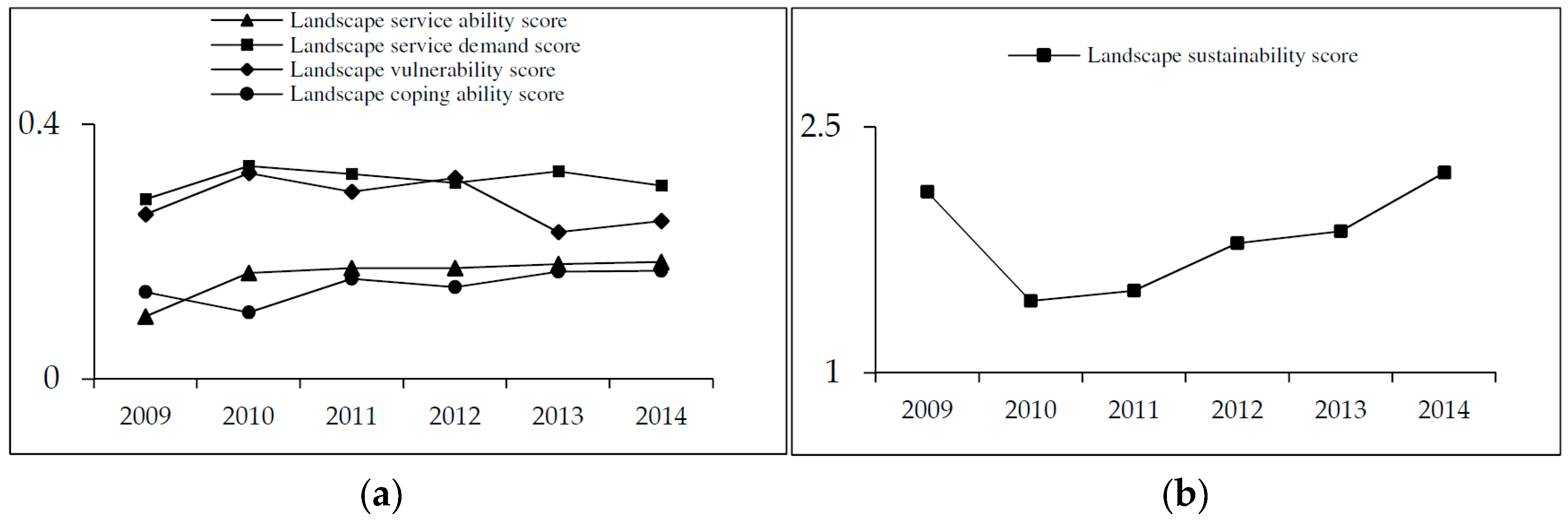
The landscape service ability score showed an upward trend from 2009 to 2014 (
Figure 1a), indicating that the supporting capacity of the rural landscape system gradually increased. The landscape service demand score showed an increasing trend during the study period, indicating that the pressure of human activities on the rural landscape system increased and that the diversity and complexity of the system increased. The overall landscape vulnerability score showed a decreasing trend and the landscape response ability increased. This pattern indicated that the vulnerability of the landscape gradually decreased during the study period and that the capacity of the rural landscape system to resist disturbance increased steadily with an increase in investments in ecological environmental protection.
The total sustainability score of the rural landscape system fluctuated upward (
Figure 1b). The year 2010 had the lowest score, and an increasing trend was observed after 2010 to obtain the highest score in 2014. The lowest score might have been obtained in 2010 due to the extreme weather disturbances that occurred that year, and the year 2014 might have shown the highest score due to continuous improvements in economic and social development and environmental management in the study area.
3.2. Entropy Change and Landscape Sustainability Analysis of Each Community
To reveal the spatial differentiation of landscape sustainability in the study area, the landscape sustainability scores of each community were analyzed in this study (
Table 3). As shown in
Table 4, although the sustainability score of Mizhi County exhibited an upward trend, the changes among the communities in the county were quite different.
There were two categories of landscape sustainability among these communities. One was the category of increased landscape sustainability and the other was the category of reduced landscape sustainability. The former included 11 communities and the latter contained two communities. In addition, the former had more obvious influence on the landscape sustainability of the study area than the latter.
There were also significant differences between the two categories of landscape sustainability. The category of increased sustainability was more complex than the category of reduced sustainability. In addition, the former could be divided into three types, namely, reduced entropy flow and entropy production, reduced entropy flow and increased entropy production and increased entropy flow and reduced entropy production, and these three types were observed in communities, three communities and three communities, respectively. The first type is the desired type of sustainability, in which attention is paid to the encouragement of landscape supportive ability. Ecological improvement is neglected to some extent in the second type and the third type is the opposite of the second type.
3.3. Spatial Differentiation of Landscape Sustainability
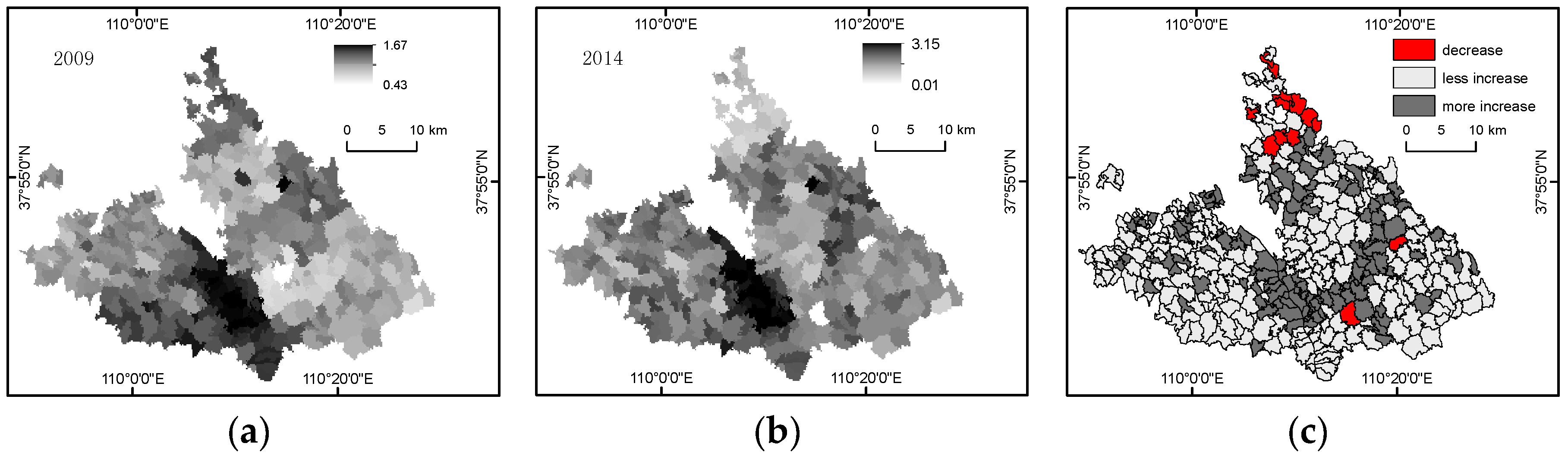
Based on Equations (7) and (8), the effects of landscape composition, landscape configuration and landscape structure on the villages in 2009 and 2014 were calculated (
Table 4), and the spatial-temporal differentiation was observed (
Figure 2).
Figure 2a,b show that villages with a high landscape sustainability score were mainly concentrated in the middle of the study area. To show the spatial and temporal differentiation of landscape sustainability, ArcGIS 10.2 was used to calculate the change in landscape sustainability by subtracting the landscape sustainability score in 2014 from that in 2009 (
Figure 2c). The landscape sustainability scores in 2014 were higher than those in 2009 for all but 11 villages (
Figure 2c), and these 11 villages were mainly located in the northeast of the study area. With the natural breaks (Jenks) method, the villages with an increasing sustainability score were divided into two categories: those with a smaller increase and those with a larger increase. The villages with a larger increase were mainly distributed in the middle of the study area.
As presented in
Table 4, several interesting results were obtained, including the following.
If the effects of landscape structure and landscape composition were not considered, the landscape sustainability score of all of the villages in Mizhi County was overestimated in 2009. Under the comprehensive influence of landscape configuration and landscape composition, the landscape sustainability score was greater than the individual influence of landscape configuration and that of landscape composition in 2009. The landscape composition’s effect was stronger than the landscape configuration’s effect.
If the effects of landscape structure and landscape composition were not considered, the landscape sustainability score of 87% of the villages was overestimated and that of 13% of the villages was underestimated in 2014. As in 2009, the landscape sustainability score was greater than the individual influence of landscape configuration and that of landscape composition in 2014. Unlike in 2009, the landscape composition’s effect was weaker than the landscape configuration’s effect in 2014.
4. Discussion
The index system based on entropy effectively reflected the structure, function and mechanism of the evolution of complex landscape ecosystems, enriching the body of research on the use of index systems in the evaluation of landscape sustainability. By considering the change in the entropy of each subsystem, the landscape sustainability evaluation index system that was constructed in this paper provides an effective method for better understanding the evolution and sustainability of the complex ecosystem of the landscape in the study area, and analyses of landscape sustainability in similar areas were also performed. However, this method alone was not enough to express the spatial differentiation of landscape sustainability.
This study has two main objectives based on the selected landscape composition and configuration indicators: one objective was to analyze and discuss the quantitative influence of changes in the landscape structure on the spatial differentiation of landscape sustainability, and the other was to explore and analyze the different effects of the landscape composition and configuration on landscape sustainability. As with similar studies, this paper found that evaluation results can be overestimated if the influence of the landscape structure is not considered [
35,
36]. However, unlike in other similar studies, in this study, the effect of landscape composition was greater than that of landscape configuration on landscape sustainability in most of the villages that were examined, and the effect of the landscape components of some villages on their landscape sustainability was greater than that of their landscape configuration [
33,
37]. Such differences might be related to the selection of indicators, the number of indicators and the quantitative expression of the effect of indicators. Therefore, to reveal the effect of landscape structure on landscapes in terms of spatial and temporal differentiation of sustainability, research studies should urgently study the effect of different landscape composition indicators and landscape configuration indicators on landscape sustainability and compare the quantitative expression of different indices. The study of the landscape based on Boltzmann entropy provides a feasible way to explore the influence of landscape structure and composition on the sustainability of the landscape. At present, the landscape research based on Boltzmann entropy has been developed from theoretical exploration to case study and its quantitative method has been effectively improved [
22,
23]. In this paper, although the sustainable spatial differentiation of the landscape is represented by improving information entropy and combining with specific landscape index, the validity has not been verified effectively. As Boltzmann entropy can effectively represent the influence of landscape structure and composition on the landscape entropy [
23], the analysis of landscape sustainability through Boltzmann entropy also provides a new way to test and verify the research results in this paper. This is one of the author’s main research tasks in the future.
The land-use pattern of the study region has been affected by policies [
38,
39]. Moreover, these policies have affected the landscape service capacity, the demand for landscape services, the landscape vulnerability and the landscape response ability. Therefore, policies can have great impacts on regional landscape sustainability. A main research task in the future will be to explore the impact of policies on regional landscape sustainability.
5. Conclusions
Based on entropy, a landscape sustainability index system was constructed in this paper. In addition, the evolution of a complex landscape ecosystem in the study area was discussed and analyzed. Finally, a spatial and temporal analysis of landscape sustainability was performed in combination with an analysis of landscape indicators. Several conclusions such as the following were drawn.
Entropy change analysis could be used to evaluate landscape sustainability. Combined with time series analysis, entropy change analysis is helpful for introducing specific measures to solve the problems that are not conducive to landscape sustainability in each subsystem.
The analysis of landscape entropy change revealed that the carrying capacity of the complex ecosystem in the study area was increasing and that the complex ecosystem developed in a healthy and orderly manner.
If the effect of landscape structure is not considered, the landscape sustainability of the study area might be overestimated, and the effect of landscape structure on landscape sustainability was greater than that of landscape component indicators or single landscape configuration indicators alone. Furthermore, for most villages in the study area, the effect of landscape composition on landscape sustainability is greater than that of landscape configuration on landscape sustainability.
Author Contributions
X.L., H.J. and H.C. designed the research and wrote the paper. D.L. and H.Z. analyzed the data. All of the authors read and approved the final manuscript.
Funding
This research was funded by the National Science Foundation of China grant number [No. 41671086, 41271103] And The APC was funded by [No. 41671086]
Acknowledgments
The authors would like to thank Ji Siwen for his untiring help in the field and the valuable advices from anonymous reviewers.
Conflicts of Interest
The authors declare no conflict of interest.
References
- Musacchio, L.R. The scientific basis for the design of landscape sustainability: A conceptual framework for translational landscape research and practice of designed landscapes and the six Es of landscape sustainability. Landsc. Ecol. 2009, 24, 993–1013. [Google Scholar] [CrossRef]
- Wu, J. A landscape approach for sustainability science. In Sustainability Science: The Emerging Paradigm and the Urban Environment; Weinstein, M.P., Turner, R.E., Eds.; Springer: New York, NY, USA, 2012; pp. 59–77. [Google Scholar]
- Li, B.L.T.; Janetos, A.C.; Verburg, P.H.; Murray, A.T. Land system architecture: Using land systems to adapt and mitigate global environmental change. Glob. Environ. Chang. 2013, 23, 395–397. [Google Scholar]
- Turner, M.G.; Donato, D.C.; Romme, W.H. Consequences of spatial heterogeneity for ecosystem services in changing forest landscapes: Priorities for future research. Landsc. Ecol. 2013, 28, 1081–1097. [Google Scholar] [CrossRef]
- Wu, J. Landscape sustainability science: Ecosystem services and human well-being in changing landscapes. Landsc. Ecol. 2013, 28, 999–1023. [Google Scholar] [CrossRef]
- Coelho, P.; Mascarenhas, A.; Vaz, P.; Dores, A.; Ramos, T.B. A framework for regional sustainability assessment: Developing indicators for a Portuguese region. Sustain. Dev. 2010, 18, 211–219. [Google Scholar] [CrossRef]
- Palomo, I.; Montes, C.; Martín-López, B.; González, J.A.; García-Llorente, M.; Alcorlo, P.; García Mora, M.R. Incorporating the social-ecological approach in protected areas in the anthropocene. Bioscience 2014, 64, 181–191. [Google Scholar] [CrossRef]
- Janssen, M.; Bodin, R.; Anderies, J.M.; Elmqvist, T.; Ernstson, H.; McAllister, R.J.; Olsson, P.; Ryan, P.; Bodin, O. Toward a network perspective of the study of resilience in social-ecological systems. Ecol. Soc. 2006, 11, 1599–1604. [Google Scholar] [CrossRef]
- Biggs, R.; Schluter, M.; Biggs, D.; Bohensky, E.L.; BurnSilver, S.; Cundill, G.; Dakos, V.; Daw, T.M.; Evans, L.S.; Kotschy, K.; et al. Toward principles for enhancing the resilience of ecosystem services. Annu. Rev. Environ. Resour. 2012, 37, 421–448. [Google Scholar] [CrossRef]
- Slootweg, R.; Jones, M. Resilience thinking improves SEA: A discussion paper. Impact Assess. Proj. Apprais. 2011, 29, 263–276. [Google Scholar]
- Nowak, A.; Grunewald, K. Landscape sustainability in terms of landscape services in rural areas: Exemplified with a case study area in Poland. Ecol. Indic. 2018. [Google Scholar] [CrossRef]
- Zhou, Z.Y.; Duan, J.N.; Liang, C.F. Temporal and spatial variation of land use structure based on information entropy in Changsha. Econ. Geogr. 2012, 32, 124–129, (In Chinese with English Abstract). [Google Scholar]
- Shannon, C.E. A mathematical theory of communication. Bell Syst. Tech. J. 1948, 27, 379–423. [Google Scholar] [CrossRef]
- Balocco, C.; Grazzini, G. Thermodynamic parameters for energy sustainability of urban areas. Solar Energy 2000, 69, 351–356. [Google Scholar] [CrossRef]
- Herrmann-Pillath, C.; Kirchert, D.; Pan, J. Disparities in Chinese economic development: Approaches on different levels of aggregation. Econ. Syst. 2002, 26, 31–54. [Google Scholar] [CrossRef]
- Geng, H.Q.; Gu, S.Z.; Gou, D.M. Analyses on evolution of household energy consumption structure based on information entropy. J. Nat. Resour. 2004, 19, 257–262, (In Chinese with English Summary). [Google Scholar]
- Zhang, Y.; Yang, Z.F.; Li, W. Analyses of urban ecosystem based on information entropy. Ecol. Model. 2006, 197, 1–12. [Google Scholar] [CrossRef]
- Svirezhev, Y.M. Thermodynamics and ecology. Ecol. Model. 2000, 132, 11–22. [Google Scholar] [CrossRef]
- Qiao, J. Application of improved entropy method in Henan sustainable development evaluation. Resour. Sci. 2004, 26, 113–118, (In Chinese with English Summary). [Google Scholar]
- Cushman, S.A. Thermodynamics in landscape ecology: The importance of integrating measurement and modeling of landscape entropy. Landsc. Ecol. 2015, 30, 7–10. [Google Scholar] [CrossRef]
- Vranken, I.; Baudry, J.; Aubinet, M.; Visser, M.; Bogaert, J. A review on the use of entropy in landscape ecology: Heterogeneity, unpredictability, scale dependence and their links with thermodynamics. Landsc. Ecol. 2015, 30, 51–65. [Google Scholar] [CrossRef]
- Gao, P.C.; Zhang, H.; Li, Z.L. A hierarchy-based solution to calculate the configurational entropy of landscape gradients. Landsc. Ecol. 2017, 32, 1133–1146. [Google Scholar] [CrossRef]
- Gao, P.C.; Zhang, H.; Li, Z.L. An efficient analytical method for computing the Boltzmann entropy of a landscape gradient. Trans. GIS 2018, in press. [Google Scholar] [CrossRef]
- Chen, H.; Marter-Kenyon, J.; López-Carr, D.; Liang, X.Y. Land cover and landscape changes in Shaanxi Province during China’s Grain for Green Program (2000–2010). Environ. Monit. Assess. 2015, 187, 1–14. [Google Scholar] [CrossRef] [PubMed]
- Liu, L.M. A study on soil erosion and land use planning with remote sensing in the hill and guliy region of the Loess Plateau: A case study in Mizhi County, Shanxi Province. J. Nat. Resour. China 1992, 7, 361–371, (In Chinese with English Abstract). [Google Scholar]
- Ministry of Water Resources of the People’s Republic of China. Sl190-2007 Standards for Classification and Gradation of Soil Erosion; China Water and Hydropower Press: Beijing, China, 2008; pp. 3–12. (In Chinese)
- Weber, B.H.; Depew, D.J.; Smith, J.D. Entropy Information and Evolution: New Perspectives on Physical and Biological Evolution; MIT Press: Cambridge, MA, USA, 1988; p. 173. [Google Scholar]
- Zhao, W.W.; Fang, X.N. Sustainable landscapes and landscape sustainability science. J. Ecol. 2014, 34, 2453–2459. [Google Scholar]
- Fang, X.N.; Zhao, W.W.; Fu, B.J. Landscape service capability, landscape service flow and landscape service demand: A new framework for landscape services and its use for landscape sustainability assessment. Prog. Phys. Geogr. 2015, 39, 817–836. [Google Scholar] [CrossRef]
- Koniak, G.; Noy-Meir, I.; Perevolotsky, A. Modelling dynamics of ecosystem services basket in Mediterranean landscapes: A tool for rational management. Landsc. Ecol. 2011, 26, 109–124. [Google Scholar] [CrossRef]
- Wu, T.; Kim, Y.S. Pricing ecosystem resilience in frequent fire ponderosa pine forests. For. Policy Econ. 2013, 27, 8–12. [Google Scholar] [CrossRef]
- Mitchell, M.G.E.; Bennett, E.M.; Gonzalez, A. Strong and nonlinear effects of fragmentation on ecosystem service provision at multiple scales. Environ. Res. Lett. 2015, 10, 094014. [Google Scholar] [CrossRef]
- Verhagen, W.; Teeffelen, A.J.A.V.; Compagnucci, A.B.; Poggio, L.; Gimona, A.; Verburg, P.H. Effects of landscape configuration on mapping ecosystem service capacity: A review of evidence and a case study in Scotland. Landsc. Ecol. 2016, 31, 1457–1479. [Google Scholar] [CrossRef]
- Chen, H.; López-Carr, D.; Tan, Y.; Liang, X.Y. China’s Grain for Green policy and farm dynamics: Simulating household land-use responses. Reg. Environ. Chang. 2016, 16, 1147–1159. [Google Scholar] [CrossRef]
- Lautenbach, S.; Kugel, C.; Lausch, A.; Seppelt, R. Analysis of historic changes in regional ecosystem service provisioning using land use data. Ecol. Indic. 2011, 11, 676–687. [Google Scholar] [CrossRef]
- Frank, S.; Fürst, C.; Koschke, L.; Witt, A.; Makeschin, F. Assessment of landscape aesthetics-validation of a landscape metrics-based assessment by visual estimation of the scenic beauty. Ecol. Indic. 2013, 32, 222–231. [Google Scholar] [CrossRef]
- Lamy, T.; Liss, K.N.; Gonzalez, A.; Bennett, E.M. Landscape structure affects the provision of multiple ecosystem Services. Environ. Res. Lett. 2016, 11, 124017. [Google Scholar] [CrossRef]
- Zhong, T.; Mitchell, B.; Scott, S.; Huang, X.; Li, Y.; Lu, X. Growing centralization in China’s farmland protection policy in response to policy failure and related upward-extending unwillingness to protect farmland since 1978. Environ. Plan. C 2017, 35, 1075–1097. [Google Scholar] [CrossRef]
- Treacy, P.; Jagger, P.; Song, C.; Zhang, Q.; Bilsborrow, R.E. Impacts of China’s Grain for Green Program on Migration and Household Income. Environ. Manag. 2018, 62, 489–499. [Google Scholar] [CrossRef] [PubMed]
© 2018 by the authors. Licensee MDPI, Basel, Switzerland. This article is an open access article distributed under the terms and conditions of the Creative Commons Attribution (CC BY) license (http://creativecommons.org/licenses/by/4.0/).


