Resampling Techniques for Real Estate Appraisals: Testing the Bootstrap Approach

Abstract

Applied to real estate markets analysis, the resampling methods aim to contribute to the knowledge growth of real estate market dynamics, overcoming the issues related to the data scarcity and operational limits of traditional statistical theory. Among resampling methods, the Bootstrap technique appears to be the most suitable for the interpretation of real estate phenomena. In this study, for residential properties located in Cosenza (Calabria Region, Italy), a Bootstrap approach has been used in order to determine the marginal prices of the real estate characteristics detected, comparing the results with those obtainable with a traditional Multiple Regression Analysis.

1. Introduction

In the presence of a sufficient amount of real estate data, the traditional statistical theory postulates a normal distribution for the real estate prices, consequently requiring the adoption of specific statistical measures applicable to the data population (e.g., mean, median, variance, standard error, standard deviation, etc.). However, in the real estate field, there is usually a low amount of detectable real estate data: this circumstance, together with the stratification processes of real estate markets, are conditions that do not satisfy the postulate of a normal distribution of the observed real estate prices [1,2,3,4,5,6,7,8,9,10,11,12].

From a general and statistical point of view, for Multiple Regression Analysis (MRA), it must be considered that the distribution of the independent variables (real estate characteristics) is irrelevant if the assumptions of homoscedasticity and normality are fulfilled for the residuals. Non-normally distributed dependent variables are hard to contrive for situations where there is a real effect on the data and the residuals are normally distributed. For a real effect on the data, dependent variables (e.g., real estate prices) might often follow a Gaussian distribution, but this does not in any way imply that Gaussianity of dependent variables is necessary for the MRA to work [13].

In multivariate analysis applied for estimative purposes, the “determination index” is a useful indicator for understanding the reliability level of real estate values estimated; in fact, this index expresses the adaptation goodness of the estimation function to the observed real estate data. With regards to the estimation function, it is assumed as the best interpolating function of the real estate sample, as well as (by generalization) for the entire real estate data population. However, it is clear that this hypothesis disregards the possibility of “deviation” (or variability) of the estimation function with respect to the statistical distribution of the comparable properties universe [14,15].

The variability of the estimation function can be investigated, in practice, by determining the confidence intervals for the determination index or regression coefficients (real estate marginal prices). At the same time, however, it is also necessary to have many real estate samples, different from the sample used to construct the estimation function, while the typical conditions of estimative practice only allow for a single real estate sample with a small size.

The resampling methods applied to the real estate market allow appraisals with a small dataset to be implemented and the postulate of normal distribution of the real estate prices to be overcome and, thus, these methods are able to produce relevant improvements in the statistical-estimative analysis usually executable in this field [2,3,4,5,6,7,8,9,10,11,12].

Bootstrap (or Bootstrapping) is a particular technique that falls in the broader class of resampling methods, and it relies on random sampling with replacement and allows measures of accuracy (defined in terms of variance, prediction error, bias, confidence intervals, etc.) to be assigned to sample estimates. This technique allows an estimation of the sampling distribution of almost any statistic using random sampling methods. Bootstrap is the practice of estimating properties of an estimator (such as its variance) by measuring those properties when sampling from an approximating distribution. Often, it is used as an alternative to statistical inference based on the assumption of a parametric model when that assumption is in doubt, or where parametric inference is impossible or requires complicated formulas for the calculation of standard errors [16].

2. Targets and Research Design

Bootstrap has wide potentialities in the real estate field and presents some relevant advantages, especially from a practical point of view, with it being easy to apply and able to derive the estimates of standard errors and confidence intervals for complex estimators of complex parameters of the distribution [16].

Starting from the literature review, it derives that Bootstrap applications in the real estate sector or for appraisal purposes are very scarce in the international reference literature, and there is nothing in the Italian real estate field. It should also be considered that the Italian real estate market is traditionally characterized by opacity and a reduced availability of data. Hence the research question of this study relates to testing and experimenting with the Bootstrap technique for an Italian real estate market using a more robust model than traditional multiparametric methods.

For these reasons, in this work, a Bootstrap approach was applied to a housing market segment with the aim of determining the marginal prices of the real estate characteristics detected, and the results of the Bootstrap application were then compared with those obtained from a traditional MRA. The purpose of this comparison is to verify the reliability of the Bootstrap technique for real estate appraisals and to show its forecasting potentialities in housing markets analysis.

MRA has been chosen for comparison purposes since it is a well-established methodology over time that provides robust and reliable results in real estate appraisals.

The analysis is carried out through the elaboration of real estate prices of housing units located in a central urban area of Cosenza (Calabria Region, Italy).

Due to data scarcity and the opacity of Italian real estate markets, in an effective manner, the Bootstrap approaches can aid in better interpreting different segments of local real estate markets, or even the prediction and interpretation of the phenomena related to the genesis of rewards of position, with particular reference to problems of transformation and investments for urban areas affected by particular projects or plans, and in order to optimize the choices of use of goods and resources.

3. Literature Review

The resampling methods include a wide class of statistical techniques, among which the most common are Jackknife, Bootstrap, and Cross-Validation [16,17,18,19,20].

These techniques are based on the logic of simulation, but they are different from a conceptual point of view because all inferential decisions derive directly from the original sample. Also, these techniques are non-parametric methodologies and are mainly aimed at measuring the goodness, in terms of variability, of an estimated value (starting from the observed data). By their nature, therefore, they allow researchers to “reuse” the only real estate sample available in order to generate “with repetitions” a wide number of further samples, useful for determining the variability degree of the estimated value in relation to the data population.

In statistics, a Bootstrap technique (or Bootstrapping) is any test or procedure that relies on random sampling with replacement [21]. Then, the technique in question allows the estimation of sampling distribution of almost any statistic using random sampling methods [22,23]. The Bootstrap technique was proposed by Efron [17], inspired by earlier works on the Jackknife [24,25,26]. Improved estimates of the variance were developed later [27,28]. A Bayesian extension of the Bootstrap technique was developed in 1981 by Efron and Stein [29]. A particular Bias-Corrected and Accelerated Bootstrap procedure was developed by Efron in 1987 [30]. Later, in 1992, Diciccio and Efron implemented the Bootstrap procedure developing a dependable algorithm for calculating highly accurate approximate intervals on a routine basis [31].

Bootstrap applications in the real estate sector or for appraisal purposes are not often included in the international reference literature. Among the most relevant studies: Kuhle and Moorehead consider a Bootstrap approach for the determination of the real estate cap rate [32]; Chi-Wei et al. apply the Bootstrap Panel Granger causality test to examine the relationship between housing prices and GDP for several provinces in China [33]; Liu et al. apply the Bootstrap Panel Granger causality test to examine the relationship between urbanization and real estate investment from 1990 to 2014 for 29 provinces in China [34]; Atkins et al. use the Monte Carlo simulation and Bootstrap technique to investigate, using traditional asset classes, the effectiveness in managing the long-term risks associated with future real estate purchases [35]; even through a Bootstrapping distribution, Gallin uses standard error-correction models and long-horizon regression models to examine how well the rent-price ratio predicts future changes in real estate rents and prices [36]; Brasington and Hite compare the performance of a mixed model to a hedonic model that includes characteristics of the buyer of each house [37]; Fingleton proposes a new GMM estimator for spatial regression models with moving average errors [38]; and Greiner and Thomas examine the possibilities and boundaries of the sample-based valuation of residential real estate portfolios using an upstream principal component and cluster analysis in Germany [39]. The cases examined all show that the Bootstrap technique is a robust statistical procedure that is not very sensitive to small or moderate deviations (in terms of data distribution) from the hypothesised model. Two concepts of robustness can be distinguished: (1) robustness with respect to contamination (outliers); and (2) robustness compared to incorrect specification (misspecification). The first concept wants to take into account, in the statistical model and in the inference, the possible presence of anomalous data in the sample, i.e., some fraction of observations that are not actually representative of the population under study. These anomalous data may be caused by detection or coding errors, but also by a slight heterogeneity of the population. Additionally, the problems resulting from the discretization, caused by the rounding of values or the reduction in classes, can be treated in this area. The second concept of robustness wishes to preserve inference procedures based on a conventional specification of the statistical model, from the plausible inadequacy of the model as an exact model. In other words, the statistical model, while qualitatively and quantitatively capturing important aspects of the data, in particular those on which it is desired to make an inference, due to its approximate character, does not accurately describe all aspects of the variability of the population [40,41,42].

These two different aspects of robustness, although conceptually distinct, are nevertheless very close and in many cases equivalent from a practical point of view. In fact, an incorrect specification of the model can be the cause of the presence of anomalous data in the observed sample; that is, of observations distant from the majority of the data. However, empirical experience has shown that even the best techniques for eliminating abnormal observations always work less well than robust inference techniques, which can be a very important aspect, especially in the real estate field [40,42].

4. Methodology

Among resampling methods, the Bootstrap procedure is the most suitable for real estate appraisals. It is conceptually simple, being mainly aimed at the non-parametric estimation of the statistical error (standard deviation or bias of the estimator), or at the evaluation of the accuracy degree of an estimator $\hat{\mathsf{\theta }}$ for a specific parameter $\mathsf{\theta }$.

Proposed for the first time by Efron [17], the Bootstrap technique represents a generalization of the Jackknife procedure. The Jackknife (or leave-one-out) procedure was proposed by Quenouille in 1949 [43] and is based on the removal of samples from the available data group and the subsequent recalculation of the estimator. It was introduced and used for a long time essentially to reduce or eliminate the bias present in some estimators, was then extended to estimate the variance of estimators, and was finally applied for the construction of confidence intervals [16].

Bootstrap is basically a resampling procedure used to provide numerical solutions to problems whose complexity makes the use of traditional statistical analysis unattainable. The application of the procedure itself is justified in all concrete situations in which the classical methods of inference operate under very restrictive or unrealistic hypotheses or “in asymptotic terms”.

However, it is necessary to consider that Bootstrap procedures raise algorithmic issues (which may be resolved with appropriate IT tools only), but also interpretative difficulties regarding the reliability/variability of the results.

4.1. Analytical Aspects of Bootstrap Approach

The main aspect characterizing a Bootstrap procedure is the possibility it offers to estimate unknown values of the population based on the only available sample.

During the elaboration process, it is assumed that the random variable R(X, F) depends on the behaviour of the X character in the population and on the corresponding unknown distribution function F. Another assumption is the possibility to identify the distribution law of R on the basis of the observed data relative to a single statistical sample. In line with these assumptions, not having any information about the F function, it is necessary:

▪

to determine the empirical distribution function $\breve{F}$ by assigning a probability of 1/n to each element of the sample (X₁, X₂, ..., X_n): from a theoretical point of view, the function of empirical distribution constitutes the non-parametric estimation of the maximum likelihood of population F;

▪

to extract a random sample with a repetition from $\breve{F}$, called the “Bootstrap sample”, with width n or consisting of n random variables ($X_i^{\ast }$) that are independent and identically distributed (i.i.d.) with the following empirical realization: (x*₁, x*₂, K, x*_n);

▪

to approximate the R(X, F) distribution with the distribution of R* = R(X*, $\breve{F}$) inducted by the random extraction mechanism of X*, with a constant $\breve{F}$ term for each extracted value.

The basis of the logical procedure is that the R* distribution, calculable once the sample has been observed, is equal to the R distribution if F = $\breve{F}$.

It is also evident that the equality between F (theoretical distribution) and $\breve{F}$ (empirical distribution) only depends on the original sample, which may contain information that makes it unlikely that $F=\tilde{F}$ will occur. It follows that the unreliability of the estimate of R through R* is considered directly dependent on the relative empirical distribution.

The most complicated phase of the procedure is the calculation of the “Bootstrap distribution”. According to Efron [17], this calculation can be performed with three different and alternative methods:

▪

the direct theoretical calculation, only usable in the simplest cases;

▪

the approximation of the Bootstrap distribution with the Monte Carlo method, where the repeated bootstrap samples are generated from the random sample with width n, extracted from $\breve{F}$, whose empirical realizations are:

x*¹ = (x₁*¹, x₂*¹, K, x_n*¹)

x*² = (x₁*², x₂*², K, x_n*²)

x*^B = (x₁*^B, x₂*^B, K, x_n*^B)

where the histogram of the corresponding values R(X* ¹,$\widehat{F}$), R(X* ²,$\widehat{F}$), K, R(X* ^B,$\widehat{F}$), is assumed as an estimation of the Bootstrap distribution;

▪

the Taylor series expansion method, approximating the mean and variance of the Bootstrap distribution of R*.

The different steps of the Bootstrap procedure can be adequately illustrated considering the classical problem for whose resolution it has been defined: the case of the bias reduction for an estimator $\mathsf{\theta }$.

In particular, considering a sample X = (X₁, X₂, K, X_N) extracted i.i.d. from an X population with an unknown F distribution function, calling $\hat{\mathsf{\theta }}$ the estimator of the $\mathsf{\theta }\left(F\right)$ parameter, the bias of $\hat{\mathsf{\theta }}$ estimator is obtainable as follows:

$$d^{\ast }\left(\hat{\mathsf{\theta }}\right)=E_F\left(\hat{\mathsf{\theta }}\right)-\mathsf{\theta }\left(F\right)$$

where all terms are completely unknown, being the unknown distribution function of the population (F).

Although unknown, the F function can be substituted by an estimate of $\widehat{F}$ based on the sampling observations. For this purpose, considering the difficulties of bias calculation, the Monte Carlo method is applicable according to the following steps:

▪

it is extracted as a Bernoullian sample $\widehat{F}$ of width n (Bootstrap sample) indicated by x*¹ = (x₁*¹, x₂*¹, K, x_n*¹), and the estimate of this sample is then carried out as follows:

$$t(x_1{}^{\ast 1}, x_2{}^{\ast 1}, K, x_n{}^{\ast 1})={\hat{\mathsf{\theta }}}_i^{\ast }$$

▪

repeat the above step for a number B of times to obtain the following estimates:

$${\hat{\mathsf{\theta }}}_1^{\ast }=\left(X_1^{\ast 1}\right),{\hat{\mathsf{\theta }}}_2^{\ast }=\left(X_2^{\ast 2}\right),K,{\hat{\mathsf{\theta }}}_B^{\ast }=\left(X_B^{\ast B}\right)$$

the latter must be used in order to obtain:

(a)

the Bootstrap estimation for $\mathsf{\theta }$:

$${\hat{\mathsf{\theta }}}_{\mathrm{Boot}}^{\ast }=\frac{1}{B}{\displaystyle \sum }_{b=1}^B{\hat{\mathsf{\theta }}}_b^{\ast }$$

(b)

the Bootstrap estimation of the bias for $\hat{\mathsf{\theta }}$:

$$d^{\ast }\left(\hat{\mathsf{\theta }}\right)={\hat{\mathsf{\theta }}}_{\mathrm{Boot}}^{\ast }-\mathsf{\theta }$$

(c)

the Bootstrap estimation of the variance for $\hat{\mathsf{\theta }}$:

$$v_B\left(\hat{\mathsf{\theta }}\right)=\frac{1}{B-1}{\displaystyle \sum }_{b=1}^B{\left({\hat{\mathsf{\theta }}}_b^{\ast }-{\hat{\mathsf{\theta }}}_{\mathrm{Boot}}^{\ast }\right)}^2$$

Furthermore, it is hypothesized that the “studentized” statistics is as follows:

$$t_B=\frac{{\hat{\mathsf{\theta }}}_{\mathrm{Boot}}-\mathsf{\theta }}{{\left[v_B\left({\hat{\mathsf{\theta }}}_n\right)\right]}^{1/2}}$$

which is asymptotically distributed as a standard normal and can therefore be used to construct appropriate confidence intervals.

From what has been explained, it is clear that the application of the Bootstrap procedure is quite easy, but the difficulties are in the choice of the value to be assigned to B. Because it is not possible to consider all the possible different Bootstrap samples, for at least one element $\left(\begin{array}{c}2n-1\\ n\end{array}\right)$, even when n is small enough, we may limit ourselves to considering an arbitrary number of them.

By way of example, it may be observed that the estimation of bias or variance requires a replication number of at least between 30 and 50, whereas it is necessary that $B\ge 1000$ for the construction of a confidence interval or carrying out a test.

4.2. Confidence Intervals of Bootstrap Approach

In the resolution of statistical inference problems, the use of traditional methods (moments method, least squares, maximum likelihood method, etc.) frequently leads to a sampling error or estimation error $\left(\hat{\mathsf{\theta }}-\mathsf{\vartheta }\right)$, due to the fact that the estimator is a function of a random sample. From this, it follows that, for each data sample, different estimations are obtainable, and moreover, the probability $\mathrm{Pr}\left(\hat{\mathsf{\theta }}=\mathsf{\vartheta }\right)$ is null if $\hat{\mathsf{\theta }}$ is a continuous random variable. Consequently, it is preferable to estimate, rather than a single value for the $\mathsf{\theta }$ parameter, a set of values (confidence interval) constructed with the probability that “covers” the true value of the $\mathsf{\theta }$ parameter with a predetermined percentage (confidence level).

The definition of adequate procedures for the determination of reliable confidence intervals is one of the most studied problems in the Bootstrap approach.

More precisely, the construction of “exact” confidence intervals is possible in very rare situations, so that only “approximate” confidence intervals can be determined more frequently.

According to the classical asymptotic theory, it can be assumed that $\left[\left(\hat{\mathsf{\theta }}-\mathsf{\theta }\right)/\mathsf{\sigma }\right]\approx N\left(0,1\right)$ is a standard confidence interval with the following form:

$$\left(\hat{\mathsf{\theta }}+z^{\mathsf{\alpha }}\hat{\mathsf{\sigma }};\hat{\mathsf{\theta }}+z^{\mathsf{\alpha }+1}\hat{\mathsf{\theta }}\right)$$

where: $\hat{\mathsf{\theta }}$ is the estimation (maximum likelihood) of the $\mathsf{\theta }$ parameter; $\hat{\mathsf{\theta }}$ is the estimation of the standard deviation of $\hat{\mathsf{\theta }}$; and $z^{\mathsf{\alpha }}$ is the α-thenth percentile of the standardized normal distribution.

The standard confidence intervals are extremely useful as they can be automatically applied to many parametric situations. However, they are very “far” from the exact ones [30]. As an alternative to the standard intervals, it is convenient to use approximate confidence intervals based on the Bootstrap procedure. The approximate confidence intervals can be constructed by the correct percentile or percentile method—used to eliminate the bias—or even by the correct accelerated percentile—which stabilizes the variance of ${\mathsf{\theta }}_n$ and simultaneously eliminates the asymmetry of the Bootstrap distribution of ${\hat{\mathsf{\theta }}}_n$ [18,30].

5. Case Study

As already mentioned, in this paragraph, the Bootstrap procedure was applied to a housing market segment of Cosenza with the aim of determining the marginal prices of the real estate characteristics detected, comparing the related results with those obtained from a traditional MRA.

For this purpose, the statistical survey concerned six different samples representative of the real estate market in many areas of Cosenza (Calabria Region, Italy). For each area, an MRA was applied to the data sample for obtaining the marginal prices of the real estate characteristics detected. Subsequently, starting from each real estate sample and area, we proceeded to “generate” 2000 Bootstrap samples, each with a width equal to the amount of data collected in each area, in order to determine the marginal prices of the real estate characteristics considered.

In this way, the Bootstrap procedure allowed us to estimate the marginal prices of the real estate characteristics for the statistical population without resorting to restrictive assumptions of the real estate prices’ distribution. This makes it possible to carry out inductive considerations about the properties of the population based on the results obtained with a unique real estate sample, and to appropriately compare the results deriving from the application of traditional statistical methodologies (MRA).

For the application of the Bootstrap technique, in accordance with the contents of paragraph 3, the hypothesis underlying the case study are the following: (a) the real estate samples extracted are independent and identically distributed (i.i.d.). Outside of this context, the bootstrap methodology involves problems of “inconsistency”, so the variability of bootstrap estimators increases with the increase of the number of bootstrap samples extracted, which can lead to incorrect estimates and therefore becomes difficult to use in the analysis of real estate data; (b) the bootstrap model will reduce the variance and, therefore, the arising of multicollinearity problems; (c) the bootstrap model will increase the determination index; and (d) the bootstrap model will be more robust (in terms of misspecification) with respect to MRA, as it is relatively insensitive to changes in the assumptions of the statistical model taking into account that a parametric model only constitutes a plausible approximation of population distribution.

5.1. Characteristics and Real Estate Market of Cosenza

Cosenza, with a population of about 70,000 inhabitants, is the capital of the homonymous province (about 730,000 inhabitants) to the north of the Calabria Region (about 1.970 million inhabitants).

The city covers an area of 37.2 sq km, at a height above sea level of 238 m.

In the last thirty years, the municipality of Cosenza has been affected by significant deurbanization: its population has decreased by about 40,000 units (−35% less inhabitants than in 1981) with the benefit of the adjacent municipalities such as Rende (+33.07% inhabitants), Castrolibero (+40% inhabitants), Mendicino (+74.62% inhabitants), Montalto Uffugo (+51% inhabitants), and Marano Principato (+129.72% inhabitants). This phenomenon was caused by the expansion of the city, mainly towards the north direction, and by a search for a better quality of life away from the chaos of the city. Together with the urban development of the district, these circumstances have favoured the creation of an integrated urban area of about 260,000 inhabitants, a polycentric form of agglomeration in which elements of physical, urban, cultural, and social continuity can be found. The disproportion between the demographic weight of the capital city and the real size of the urban area is evident. The territory has been projected for years now towards the creation of a future single municipality.

The municipal territory of Cosenza has a high rate of urbanization and is almost completely built, and this phenomenon is at the origin of the strong demographic growth of the neighboring municipalities and more generally, of the entire agglomeration. A project of integral sustainable mobility and the light rail which connects the city center with the Campus of Calabria University are under realization.

From the point of view of the real estate market, the most important urban areas are those that are central (in particular B and C, see Figure 1). Compared to the provincial scenario, about 20% of all real estate ads in the province are related to the city of Cosenza.

According to the data of the Real Estate Market Observatory of the Revenue Agency, in Cosenza, the sale price of apartments ranges between € 300/sqm and € 1750/sqm, and between 2.70 €/sqm/month and 7.50 €/sqm/month for renting. Currently, the average sale price of apartments in Cosenza (about € 1100/sqm) is about 12% higher than the average regional sale price (about € 970/sqm), and is also about 14% higher than the average provincial quotation (about € 945/sqm). Although the housing sale prices in Cosenza are not uniform, in central areas, the sale prices mainly range between € 900/sqm and € 1250/sqm. In line with the general trends of medium-sized cities located in Southern Italy, the real estate market is substantially stable. The most requested property type is represented by studio flat (mostly due to the presence of Calabria University near the city); on the contrary, the least required solutions are lofts.

5.2. Description of the Real Estate Sample

The real estate data were collected through survey forms, detecting for each real estate unit the sale price, locational characteristics (area, infrastructures), positional characteristics (building construction, number of floors, structural features, condominium technological systems, state of maintenance and conservation), typological characteristics (main surfaces, annexed and connected), number of bathrooms, panoramic views), economic data (rental situation, ownership and cadastral data), and financial data (method of financing for the purchase).

All data were collected in real estate agencies. Of 145 survey forms (housing unit sales), 16 real estate units have been deleted because they failed the verify test of trades. This test consists of verifying the similarity degree of data to the estimation sample in terms of belonging to the same real estate market segment and cross checking (buyer and seller) for the reliability of the data provided during the compilation of the survey form.

Regarding the validity of real estate data, four aspects must be considered: (1) internal validity; (2) validity of construct; (3) external validity; and (4) statistical validity.

There is “internal validity” of the real estate sample because the relationship between the independent variable and the dependent variable is causal (even in the absence of multicollinearity phenomena), so the results reflect the studied phenomenon effectively or depend on other non-considered variables (eventually included in the intercept). In general, the main factors that may threaten the “internal validity” of the sample are the errors due to the detector or the subject taken into consideration or from variables of confusion.

The “validity of construct” subsists as there is a correspondence between the research plan and the theory of reference; in fact, alternative explanations of the real estate data are excluded from the reference theory. Among the threats to the validity of constructs, the most important is the lack of identification of the phenomenon that one wants to study and its most important aspects.

The “external validity” is guaranteed by the fact of being able to extend the results to wider urban areas than the one in which the study was carried out.

On the other hand, the “statistical validity” is partially linked to the “internal validity”, as it aims to verify whether the relationship found between the experimental variables is random or not; that is, if the effect is significantly different from the one that would be obtained by chance. Statistical validity deals with checking the variability due to chance, by calculating probabilities and statistical inference. A first type of threat to statistical validity derives from “fishing”, when correlations between variables are made without having precise assumptions about them. A second type of threat to the statistical validity derives from too small samples, so that the statistical test applied does not detect a significant relationship between variables.

Then, considering the real estate sample valid under all aspects, it finally concerns n. 129 real estate units (apartments) in multi-storey buildings located in Cosenza (Calabria Region, Southern Italy), for a total of 1419 sets of data taking into account the real estate characteristics detected.

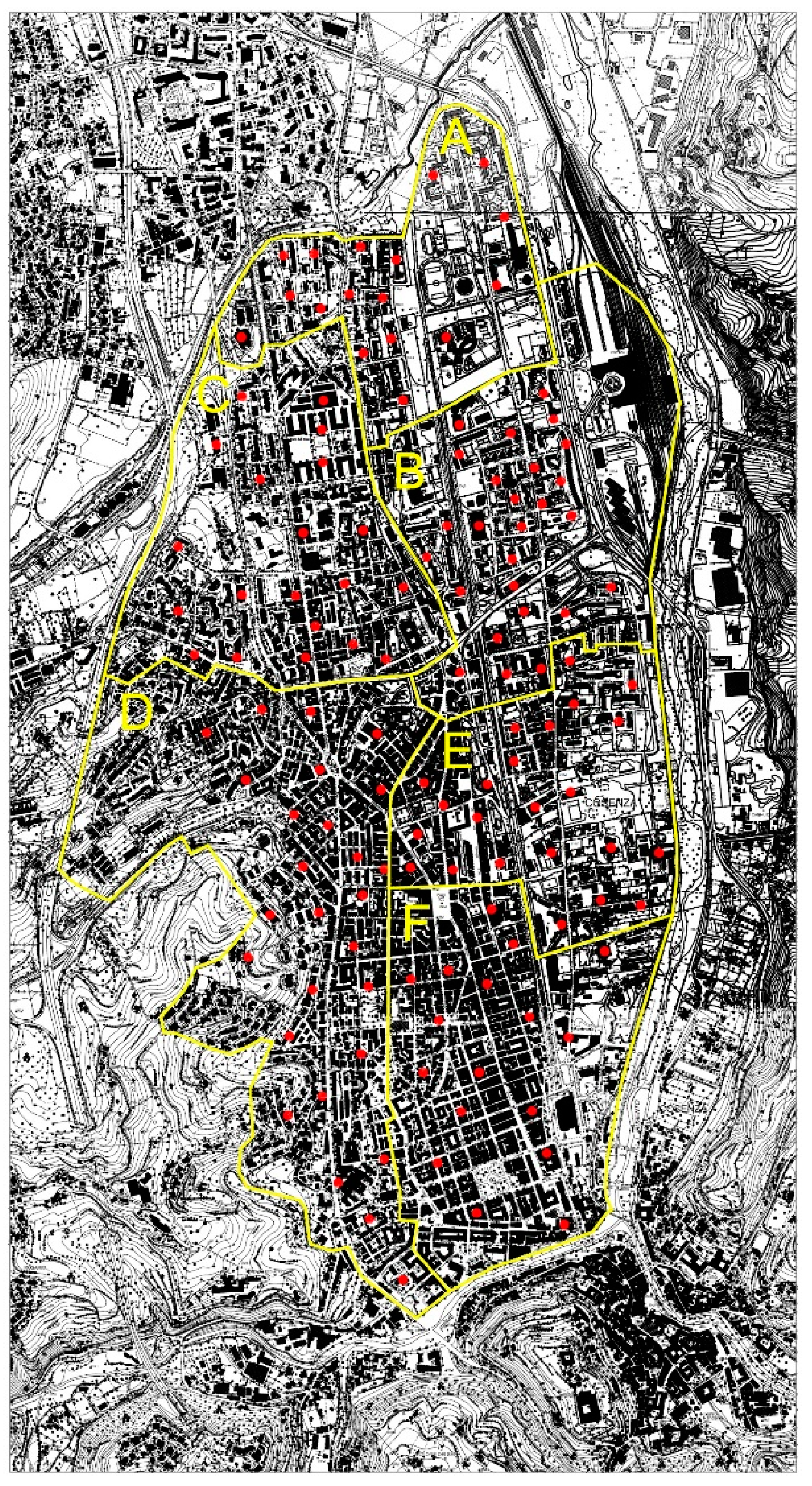
The survey did not concern the historic center of Cosenza, as well as the northern urban area where the economic-popular buildings are concentrated (mainly owned by the Territorial Company for Public Residential Construction). The real estate market for these last properties was actually non-existent during the observation period (last five years).

The survey area has been divided into six urban homogeneous areas (A, B, C, D, E, and F, see Figure 1) in order to capture the differences in terms of value determined by the different territorial distribution of the buildings. In all six urban areas considered, the building construction started from the 1950s onwards.

Zone A is located on the north side of the city; it borders the Municipality of Rende and is characterized by the presence of more recent dwellings (80s–90s).

Zone B, adjacent to zone A in a southerly direction, has a building typology whose construction period is between the 60s and the early 80s.

Zone C is located on the west side of the city and has a homogeneous building typology for construction age, construction characteristics, and maintenance status (construction period around the 50s).

Zone D, located parallel to areas E and F, has homogeneous building types whose construction date is between the 60s and the 80s.

Similarly, the south of zone E is bordering zone B and has homogeneous building types whose construction date is between the 60s and the 70s.

Zone F, located near the E zone in a southerly direction, constitutes a central part of the city and presents heterogeneous building types whose construction date is between the 50s and the 70s.

The real estate characteristics detected for each building unit are the following:

▪

purchase date (DAT), measured in years starting from the current moment;

▪

internal surface (SUI), measured in square meters, sqm;

▪

outdoor surface (SUO), measured in square meters, sqm;

▪

garage area (SUG), measured in square meters, sqm;

▪

cellar area (SUC), measured in square meters, sqm;

▪

loft surface (SUL), measured in square meters, sqm;

▪

garden outdoor area (SGA), sqm;

▪

floor level (FLOOR) of the real estate unit, level;

▪

number of views (windows/balconies) on public streets (VIEWS) of the housing unit, no.;

▪

number of bathrooms (SER) of the housing unit, no.;

▪

purchase price of real estate units (PRC), Euros.

Further real estate characteristics were excluded from the analysis as they presented themselves in the same modality for all the sampled units.

5.3. Results

Preliminarily, MRA was applied to the data sample detected in each survey area. Subsequently, the marginal prices of the real estate characteristics that could be extrapolated to the entire statistical population by means of the Bootstrap procedure were estimated.

MRA was implemented with the SPSS statistical calculation program [44]. The application of this methodology to each real estate sample made it possible to determine the marginal prices of the real estate characteristics (see

Table 1. Marginal prices of real estate characteristics (Original Sample).

Real Estate Characteristics	Zone A	Zone B	Zone C	Zone D	Zone E	Zone F
Constant	12,449.53	−9848.32	15,766.91	−16,701.18	−42,657.79	−68,843.70
DAT	−985.8	−1776.10	−2117.99	−5092.27	−2634.96	−1642.33
SUI	693.63	806.71	553.13	920.84	955.45	1267.90
SUO	177.44	240.15	359.97	437.96	472.04	276.30
SUG	173.54	221.04	-	-	-	-
SUC	226.59	-	-	-	507.68	115.17
SGA	351.36	334.66	217.94	232.92	253.06	89.35
VIEWS	279.77	525.24	470.49	2114.89	2836.38	2693.84
FLOOR	2056.77	3615.71	595.48	2040.52	2674.21	1020.00
SER	-	6126.73	2090.62	5338.10	7120.91	8602.62

) and the main statistical-estimative indexes: variance (see

Table 2. Variance (Original Sample).

Real Estate Characteristics	Zone A	Zone B	Zone C	Zone D	Zone E	Zone F
Constant	-	-	-	-	-	-
DAT	247.90	291.28	274.76	311.42	344.48	459.65
SUI	26,652.79	44.78	59,037.22	60,145.54	96,004.17	108,807.14
SUO	4191.05	19,702.83	6685.53	11,040.82	4776.71	5075.22
SUG	8686.81	45.78	-	-	-	-
SUC	6773.85	-	-	-	7643.05	9378.86
SGA	70,880.09	124,945.90	116,482.72	63,969.90	92,970.51	36,456.18
VIEWS	45.45	46.78	40.28	40.28	107.94	58.36
FLOOR	775.72	178.69	169.40	171.46	267.52	394.06
SER	-	47.78	41.32	35.64	44.93	40.28

), standard error (see

Table 3. Standard error (Original Sample).

Real Estate Characteristics	Zone A	Zone B	Zone C	Zone D	Zone E	Zone F
Constant	10,849.73	11,962.17	1646.10	14,183.46	17,488.78	21,535.74
DAT	730.79	1036.53	911.55	1187.85	1373.26	1657.31
SUI	70.24	65.59	61.97	85.73	82.12	107.94
SUO	177.66	126.02	184.89	199.35	368.75	498.90
SUG	123.43	157.00	-	-	-	-
SUC	139.96	-	-	-	291.80	366.68
SGA	43.38	50.10	44.42	83.15	83.67	185.92
VIEWS	1705.86	2638.06	2382.42	3295.51	2455.75	4657.92
FLOOR	413.17	1323.16	1161.51	1602.05	1559.18	1790.04
SER	-	2963.95	2345.75	3506.23	3810.42	5582.38

), confidence intervals (see

Table 4. Confidence intervals (Original Sample).

Real Estate Characteristics	Zone A	Zone B	Zone C	Zone D	Zone E	Zone F
Constant	[−62,048.27; 86,947.33]	[−57,903.07; 38,206.56]	[−22,521.55; 54,055.68]	[−59,603.59; 26,201.66]	[−100,157.74; 14,841.79]	[−190,879.62; 53,191.77]
DAT	[−5152.65; 3180.95]	[−5194.62; 1642.70]	[−5818.99; 1583.43]	[−8595.33; 1588.89]	[−9546.01; 4276.47]	[−8819.17; 5534.89]
SUI	[93.99; 1293.26]	[521.35; 1092.29]	[238.50; 868.21]	[635.95; 1205.81]	[523.69; 1387.47]	[735.30; 1800.39]
SUO	[−604.572; 959.45]	[−243.20; 723.85]	[−535.63; 1255.12]	[−144.72; 1020.72]	[−885.78; 1830.16]	[−2554.47; 3107.07]
SUG	[−647.59; 994.67]	[−608.68; 1050.29]	-	-	-	-
SUC	[−1142.19; 1595.38]	-	-	-	[−1510.16; 2526.01]	[−1437.25; 1667.23]
SGA	[197.93; 504.78]	[62.16; 607.44]	[6.69; 429.20]	[0.491; 465.36]	[−212.68; 718.56]	[−872.07; 1050.64]
VIEWS	[−8320.02; 8879,57]	[−8836.334; 9886.60]	[−8613.14; 9553.74]	[−7499.63; 11,729.26]	[−12,260.34; 17,933.34]	[−30,937.57; 36,325.58]
FLOOR	[91.31; 4022.22]	[−1340.60; 8572.24]	[−3533.36; 4724.45]	[−2387.14; 6468.41]	[−2526.34; 7874.50]	[−10,937.44; 12,977.16]
SER	-	[−12,773.15; 25,027.03]	[−7011.39; 11,192.16]	[−4849.46; 15,525.51]	[−10,972.82; 25,214.56]	[−18,858.50; 36,064.04]

), and determination indexes (see Table 9).

For the original sample (application or MRA), the variables’ coefficients directly express the implicit marginal prices of real estate characteristics (see Table 1):

▪

for the DAT variable, the marginal price (negative sign) ranges between €/year 958.8 (zone A) to €/year 5092.27 (Zone D);

▪

for the SUI variable, the marginal price (positive sign) ranges between €/sqm 553.13 (zone C) to €/sqm 1267.90 (Zone F);

▪

for the SUO variable, the marginal price (positive sign) ranges between €/sqm 177.44 (zone A) to €/sqm 472.04 (Zone E);

▪

for the SUG variable, the marginal price (positive sign) ranges between €/sqm 173.54 (zone A) to €/sqm 221.04 (Zone B) (this variable is not detected for C, D, E, and F Zones);

▪

for the SUC variable, the marginal price (positive sign) ranges between €/sqm 115.17 (zone F) to €/sqm 507.68 (Zone E) (this variable is not detected for B, C, and D Zones);

▪

for the SGA variable, the marginal price (positive sign) ranges between €/sqm 89.35 (zone F) to €/sqm 351.36 (Zone A);

▪

for the VIEWS variable, the marginal price (positive sign) ranges between €/no. 279.77 (zone A) to €/no. 2836.38 (Zone E) for each additional window/balcony;

▪

for the FLOOR variable, the marginal price (positive sign) ranges between €/level 595.48 (zone C) to €/level 3615.71 (Zone B) for each additional floor level;

▪

for the SER variable, the marginal price (positive sign) ranges between €/no. 2090.62 (zone C) to €/no. 8602.62 (Zone E) for each additional bathroom (this variable is not detected for A Zone).

The MRA leads to results which, for their consistency with buying and selling prices detected, can be considered representative of the validity of the methodology used.

From a statistical-estimative standpoint, the amounts of variance terms are consistent with the eligibility threshold for these values, showing no possible problems of multicollinearity between the real estate characteristics (see Table 2).

Furthermore, the amounts of standard errors are consistent with the eligibility threshold for these values, showing no noticeable abnormalities (see Table 3).

Confidence intervals show that the errors are distributed normally, and that these intervals are acceptable for the purpose of an interval estimate for the mean value of y for all units of the population with a particular value x₀ (see Table 4).

The application of the Bootstrap procedure also requires the use of appropriate IT tools and random simulation procedures. AMOS 4.0 software (Analysis of MOment Structure) was used in the present study for the random simulation processes [45].

For each urban area affected by the survey, the application of the AMOS program aimed to extract, from the original real estate sample and through reposition, 2000 Bootstrap samples with the following widths: n_A = 17 for zone A, n_B = 26 for zone B, n_C = 20 for zone C, n_D = 27 for zone D, n_E = 23 for zone E, and n_F = 16 for zone F.

The AMOS application provided the Bootstrap estimation of regression coefficients (see

Table 5. Marginal prices of real estate characteristics (Bootstrap Sample).

Real Estate Characteristics	Zone A	Zone B	Zone C	Zone D	Zone E	Zone F
Constant	13,202.19	−10,586.30	16,259.10	−16,601.00	−42,907.20	−68,989.30
DAT	−1044.28	−1804.50	−2136.58	−5116.54	−2659.24	−1709.47
SUI	690.50	807.74	548.48	917.74	954.93	1269.45
SUO	178.69	244.28	370.82	441.05	478.75	285.60
SUG	162.68	213.30	-	-	-	-
SUC	229.31	-	-	-	509.74	102.26
SGA	351.71	331.56	222.08	238.60	250.48	83.67
VIEWS	252.55	579.46	446.22	2223.35	2863.75	2836.90
FLOOR	2030.19	3688.02	609.93	2108.18	2677.83	981.78
SER	-	6451.58	2020.90	5192.97	7260.87	8593.33

), variance (see

Table 6. Variance (Bootstrap Sample).

Real Estate Characteristics	Zone A	Zone B	Zone C	Zone D	Zone E	Zone F
Constant	-	-	-	-	-	-
DAT	220.53	273.72	254.61	291.28	316.07	417.30
SUI	25,236.15	44.78	54,606.02	57,001.86	92,104.92	104,498.86
SUO	3968.97	19,083.08	6448.48	11,056.31	4610.41	4680.13
SUG	8232.84	45.78	-	-	-	-
SUC	6287.35	-	-	-	7253.12	9020.44
SGA	66,015.07	120,051.44	110,554.83	63,252.54	88,605.93	33,569.18
VIEWS	41.83	46.78	37.70	38.73	102.26	56.29
FLOOR	740.08	176.63	157.52	158.04	253.58	381.66
SER	-	47.78	38.73	34.09	42.35	37.70

), standard error (see

Table 7. Standard error (Bootstrap Sample).

Real Estate Characteristics	Zone A	Zone B	Zone C	Zone D	Zone E	Zone F
Constant	34,330.44	22,612.03	18,772.69	21,234.64	27,058.21	53,829.27
DAT	1925.87	1622.19	1799.34	1712.57	3272.79	3387.44
SUI	275.79	137.89	150.29	142.54	202.97	242.22
SUO	363.07	244.28	426.08	295.93	661.06	1255.51
SUG	380.63	412.65	-	-	-	-
SUC	626.46	-	-	-	956.99	717.36
SGA	70.24	134.28	99.68	115.17	223.11	448.80
VIEWS	3911.65	4387.82	4474.07	4720.93	7135.88	15,012.37
FLOOR	921.36	2433.55	2014.18	2180.48	2532.19	5437.77
SER	-	9150.07	4398.66	4902.73	8763.76	12,849.45

), and confidence intervals (see

Table 8. Confidence intervals (Bootstrap Sample).

Real Estate Characteristics	Zone A	Zone B	Zone C	Zone D	Zone E	Zone F
Constant	[−57,701.66; 81,829.50]	[−51,687.52; 35,559.09]	[−22,872.33; 51,259.90]	[−57,518.32; 26,848.01]	[−99,688.58; 9992.92]	[−172,625.72; 40,155.04]
DAT	[−4969.35; 2854.46]	[−4843.33; 1495.66]	[−5607.17; 1441.95]	[−8402.24; 1690.88]	[−8918.18; 3874.46]	[−8694.55; 4836.10]
SUI	[118.79; 1249.31]	[537.12; 1077.33]	[265.98; 878.49]	[650.74; 1218.32]	[551.06; 1357.25]	[766.42; 1768.86]
SUO	[−585.66; 4900.18]	[−247.38; 744.21]	[−477.72; 1186.82]	[−177.66; 1000.89]	[−915.68; 1683.65]	[−2201.66; 2749.62]
SUG	[−599.61; 955.45]	[−578.43; 1043.76]	-	-	-	-
SUC	[−1016.39; 1535.94]	-	-	-	[−1310.77; 2593.13]	[−130,302; 1601.53]
SGA	[201.42; 486.50]	[66.11; 609.94]	[8.26; 401.80]	[3.10; 453.45]	[−196.77; 675.01]	[−822.72; 997.79]
VIEWS	[−7409.09; 8321.67]	[−8491.58; 9206.88]	[−8585.06; 9479.05]	[−7801.60; 11,153.40]	[−12,567.46; 17,161.86]	[−28,580.21; 30,999.81]
FLOOR	[271.66; 3940.05]	[−1370.16; 8362.99]	[−3482.99; 4447.21]	[−2113.34; 6573.46]	[−2293.07; 7777.84]	[−10,317.26; 12,192.51]
SER	-	[−12,400.65; 23,093.37]	[−6430.92; 10,831.65]	[−3701.96; 15,086.22]	[−9937.15; 25,022.85]	[−15,146.65; 34,315.46]

).

The Bootstrap samples were generated with the Monte Carlo method, while the Bootstrap confidence intervals were calculated using the correct percentile method. With these two approaches, the calculation of the coefficients was also determined in order to compare the estimation goodness for the Bootstrap approach.

For the bootstrap sample, the implicit marginal prices of real estate characteristics are the following (see Table 5):

▪

for the DAT variable, the marginal price (negative sign) ranges between €/year 1044.28 (zone A) to €/year 5116.54 (Zone D);

▪

for the SUI variable, the marginal price (positive sign) ranges between €/sqm 548.48 (zone C) to €/sqm 1269.45 (Zone F);

▪

for the SUO variable, the marginal price (positive sign) ranges between €/sqm 178.69 (zone A) to €/sqm 478.75 (Zone E);

▪

for the SUG variable, the marginal price (positive sign) ranges between €/sqm 162.68 (zone A) to €/sqm 213.30 (Zone B) (this variable is not detected for C, D, E, and F Zones);

▪

for the SUC variable, the marginal price (positive sign) ranges between €/sqm 102.26 (zone F) to €/sqm 509.74 (Zone E) (this variable is not detected for B, C, and D Zones);

▪

for the SGA variable, the marginal price (positive sign) ranges between €/sqm 83.67 (zone F) to €/sqm 351.71 (Zone A);

▪

for the VIEWS variable, the marginal price (positive sign) ranges between €/no. 252.55 (zone A) to €/no. 2863.75 (Zone E) for each additional window/balcony;

▪

for the FLOOR variable, the marginal price (positive sign) ranges between €/level 609.93 (zone C) to €/level 3688.02 (Zone B) for each additional floor level;

▪

for the SER variable, the marginal price (positive sign) ranges between €/no. 2020.90 (zone C) to €/no. 8593.33 (Zone E) for each additional bathroom (this variable is not detected for the A Zone).

Additionally, for the bootstrap sample, the amounts of variance terms are consistent with the eligibility threshold for these values, showing no possible problems of multicollinearity between the real estate characteristics (see Table 6).

In terms of the standard errors, for the bootstrap sample, they are consistent with the eligibility threshold, showing no noticeable abnormalities (see Table 7).

Finally, for the bootstrap sample, the confidence intervals show that the errors are distributed normally, and the results obtained with the Bootstrap technique show that they are representative of the validity of the methodology used.

5.4. Results Analysis

The marginal prices calculated by applying the MRA to the original real estate sample, as well as the marginal prices obtained according to the Bootstrap procedure, show slight divergences.

In particular, higher standard errors are registered with the Bootstrap procedure, if compared to the analogous parameters obtained with the classical MRA, while the variance measurement is less high. This indicates that the oscillations of the estimated values with the Bootstrap procedure are less extensive than those obtained with the traditional MRA and therefore more reliable. Furthermore, the Bootstrap confidence intervals, for all the investigated real estate characteristics, are lower than the homologous intervals calculated for the original real estate sample. Moreover, for this reason, it can be affirmed that the Bootstrap procedure provides better results than those obtained with the traditional MRA.

Further verification that aimed to confirm the validity of the Bootstrap procedure re-examined the comparison of the determination indexes obtained with the traditional MRA.

Table 9. Determination Indexes.

Zone	R2 (Original Sample)	R2 (Bootstrap Sample)
A	0.924	0.965
B	0.897	0.933
C	0.857	0.916
D	0.853	0.893
E	0.879	0.929
F	0.905	0.957

shows that the determination indexes with the Bootstrap procedure are all better than the homologous coefficients obtained with the application of the MRA to the sample of the data collected.

For the original sample, the determination index ranges between 0.853 (D Zone) and 0.924 (A Zone); then, over 85.30% of the real estate prices variability is explained by the real estate characteristics detected. For the bootstrap sample, the determination index ranges between 0.893 (D Zone) and 0.965 (A Zone); then, in this case, over 89.30% of the real estate price variability is explained by the real estate characteristics detected.

6. Concluding Remarks

The resampling methods applied for real estate purposes allow us to overcome some limits of traditional statistical theory, obtaining statistical measures opportunely applicable to the buildings population in the presence of a small real estate data number.

The Bootstrap procedure was used in this study to analyze a real estate market segment of Cosenza (Calabria Region, Italy), and was then compared with a traditional asymptotic methodology (MRA). The results of the case study showed that the resampling methods provide more adequate measures of variance and confidence intervals for the real estate characteristics influencing the real estate prices, with a consequent improvement in the reliability level of the results obtained by the estimation.

Based on the reference literature, this paper presents the first Bootstrap application in the Italian real estate sector (typically with a low transparency) for appraisal purposes. Therefore, in light of the excellent results obtained when testing the Bootstrap technique, the initial research question can be considered widely satisfied. Also, the estimated values with the Bootstrap procedure are less extensive than those obtained with the traditional MRA and therefore they have been demonstrated to be more reliable.

Greater reliability and precision in the real estate phenomena observed, with respect to the traditional regression models, are the main results of this study, demonstrating the wide potentialities of the Bootstrap technique in the real estate field.

From an operative point of view, the variability level of the estimates obtained with the resampling methods opens interesting perspectives in distributive analysis of real estate values (considering that the territorial distribution of real estate prices is subject to considerable random variability) and for temporal dynamics of real estate prices (in order to estimate the real estate revaluation of buildings).