Housing Vulnerability and Property Prices: Spatial Analyses in the Turin Real Estate Market

Abstract

In the literature, several vulnerability/resilience indicators and indexes are based and assessed by taking into account and combining different dimensions. Housing vulnerability is one of these dimensions and is strictly related to the buildings’ physical features and to the socio-economic condition of their occupants. This research aims to study housing vulnerability in relation to the real estate market by identifying possible indicators and spatially analyzing their influence on property prices. Assuming the city of Turin and its territorial segmentation as a case study, spatial analyses were performed to take into account the presence of spatial dependence and to identify the variables that significantly influence the process of property price determination. The results of this study highlighted the fact that two housing vulnerability indicators, representative of fragile buildings’ physical features, were spatially correlated with property prices and had a significant and negative influence on them. In addition, their comparison with two social vulnerability indicators demonstrated that the presence of economical buildings and council houses was spatially correlated with the presence of people with a low education level. The results of the spatial regression model also confirmed that one of the social vulnerability indicators had the highest and most negative explanatory power in the property price determination process.

1. Introduction

The vulnerability and resilience of cities and territories are widely studied in order to measure the risk of an area being exposed to natural and manmade hazards or its capability to return to its original condition after a disaster. In the literature, several vulnerability/resilience indicators and indexes are based and assessed by taking into account and combining different dimensions. Housing vulnerability is one of these dimensions and is strictly related to the buildings’ physical features and to the socio-economic and living condition of their occupants. In the literature, the concept of housing vulnerability is mainly associated with the risk of environmental disasters, while its correlation with the variability of property prices is scarcely investigated. Therefore, in this study, an innovative perspective is assumed, according to which the concept of housing vulnerability is defined as the condition of an urban area to be impacted by the increasing gap between higher and lower property values, social marginalization and the exit from the market of entire portions of the built environment of the city. These aspects represent structural changes in the city and in its real estate market that tend to worsen during negative economic trends.

It is possible to define three types of risk to which the territorial areas of a city can be exposed: social risk, real estate market risk and risk in the built environment. Social risk is here related to the increase of the concentration of the most fragile sectors of the population, high crime levels, depopulation and a lack of the “mixitè sociale”. Real estate market risk is here related to the decrease of property prices, the extension of bargaining timing, the increase of unsold housing units, real estate depreciation and the reduction of public and private investors. Built environmental risk is here related to the increase of the number of abandoned buildings, physically deteriorated buildings and public spaces and by the lack of restoration or retrofit interventions. These kinds of risk can significantly differ among the urban areas and differently influence the related sub-markets of a city. In this paper, the real estate market risk and the presence of buildings with fragile physical features are analyzed and their influence on property prices is investigated in order to highlight those characteristics that are able to affect not only the vulnerability of the related buildings, but also the vulnerability of the urban areas where they are located and the specific real estate submarkets.

Therefore, housing vulnerability needs to be assessed and its relation with property prices has to be spatially analyzed by considering both the physical and socio-economic context. Several studies have analyzed social vulnerability, including the housing dimension [1,2,3,4,5], and have investigated the presence of spatial correlation [6,7,8,9]. Nevertheless, in the literature, at least to our knowledge, there are no investigations that study social vulnerability including the housing dimension and at the same time the presence of a spatial correlation in relation to the real estate market.

The purpose of this paper is twofold. Firstly, it aims to study housing vulnerability in relation to the real estate market by identifying three possible indicators and spatially analyzing their influence on property prices. Secondly, it aims to compare the identified housing vulnerability indicators with two social vulnerability indicators, representative of fragile sectors of the population, which a previous study demonstrated to be spatially correlated with property prices and have a significant and negative influence on them [10]. The city of Turin and its territorial segmentation into statistical zones is assumed as a case study, and widely recognized spatial dependence analyses and spatial regression models are performed [11].

The results of this study highlighted the fact that two housing vulnerability indicators, representative of fragile buildings’ physical features, were spatially correlated with property prices and had a significant and negative influence on them. In addition, their comparison with two social vulnerability indicators demonstrated that the presence of economical buildings and council houses was spatially correlated with the presence of people with a low education level. The results of the spatial regression model also confirmed that one of the social vulnerability indicators had the highest and most negative explanatory power in the property price determination process. Furthermore, this research led to the identification of the most vulnerable urban clusters characterized by low property prices, low-quality buildings and the presence of inhabitants with a low education level. Therefore, these spatial analyses can support public administrations to steer their policies by promoting new public and private investments and fostering an integrated social and territorial welfare.

The paper proceeds as follows: Section 2 introduces the background of the analysis, and Section 3 presents the methodology. The case study is introduced in Section 4, while Section 5 discusses the results. The final section presents conclusions.

2. Background

The concept of vulnerability is widely studied in the literature, with very different approaches facing various risk typologies related to natural and manmade hazards [12,13,14,15]. In particular, social vulnerability is most often described by analyzing several variables that can be linked to different dimensions; for example, a population’s social and economic condition, education, ethnicity, housing stock, urban services and infrastructures, level of urbanization and the characteristics of the built environment. In this study, particular attention is paid to exploring the dimension of housing vulnerability by analyzing the residential building stock and by identifying those features that can negatively influence the property price determination process. It is assumed that property prices are mostly related to a building’s location, but also physical and energy features, neighborhood characteristics and location amenities have a significant role in the price determination process. The physical features that play a principal role are the building’s construction period, the building’s condition and the building’s quality [16]. The latter is often a direct consequence of the building’s construction period and of the technologies and materials utilized [16].

As commonly recognized, property price data are spatial data, and it is commonly observed that spatial data are rather dependent on other factors; i.e., the observations from one location tend to exhibit values similar to those from nearby locations [17]. Consequently, the real estate market may be affected by the spatial autocorrelation of property price [6,7]. Spatial dependence arises in cross-sectional data whereby the correlation occurs among contiguous units [8,9]. For these reasons, in this study, spatial analyses and spatial regression are carried out.

2.1. Housing Vulnerability

The characteristics related to the housing stock that contribute to assessing the vulnerability of a city or an urban area are identified differently and specified on the basis of the specific territorial context. Several studies analyze those characteristics as variables used to construct vulnerability/resilience indexes [3,12,18,19,20]. Some variables are strictly related to the specific territorial context of the analysis, while others are used across various countries, even if the socio-economic and territorial contexts are obviously different. Nevertheless, those variables, even if differently defined, can foster very similar processes.

The housing condition is widely studied in order to measure the adequacy of a building to resist hazards: [18], for example, considering the percentage of precarious lodgings, while other studies observe the level of use in order to measure the percentage of vacant housing units [18,21]. The housing construction period is another characteristic which is analyzed in the literature with different specifications according to the analyzed context. The presence of new apartments was shown to be a positive indicator in the assessment of German counties in [19]. The percentage of housing units not built before 1970 and after 1994 are positively assessed by [21] who analyzed the Southeastern United States, while [18] differently considered residential constructions built in different periods of time across 78 municipalities in the Central Region of Portugal. It is worthy of mention that the presence of old houses can both negatively and positively influence the vulnerability evaluation; thus, it is fundamental to analyze this variable in conjunction with the building quality and the related historical and cultural value. Therefore, in many cases, the housing type is also investigated: for example, studies developed in the US negatively assessed the presence of mobile homes [12,14,21] and multi-unit structures [14]. Another variable, strictly related both to the housing type characteristics and to the social condition, is overcrowding in housing. Several studies consider this with different indicators: the number of persons per household is considered by [1,3,19], while [14,18,20] measured the percentage of overcrowded housing units.

Finally, considering the aim of this study, it is important to highlight the evidence in the literature regarding the influence of property prices in the vulnerability assessment. The real estate market conditions are taken into consideration by [1,2,3,4,5], who analyzed the rent/property values among the vulnerability indicators.

2.2. Spatial Analyses for Real Estate Prices

In the real estate market, building features play a crucial role in the price determination process and affect the “location similarity”, which causes the presence of spatial autocorrelation [22]. The causes of spatial autocorrelation are numerous: firstly, properties in close proximity tend to have similar structural characteristics, such as square meter living areas, dwelling age and design features. This refers to the building quality [23]. Proximate properties tend to be developed at the same time and the similar quality of the buildings may be a natural consequence of this [8,24]. Secondly, residents in the same neighborhood may follow similar commuting patterns [24], suggesting similar accessibility conditions. Thirdly, according to [6,24], property values in the same neighborhood capitalize on shared location amenities [8].

In real estate research, spatial autocorrelation is studied for the statistical improvements that can be gained by managing it in hedonic modelling [8,25]. According to [22], a crucial issue in the definition of spatial autocorrelation is the notion of “location similarity”, or the determination of those locations called “neighbors”, for which the values of the random variable are correlated. In the context of this paper, spatial autocorrelation refers to a situation where the ordinary least squares (OLS) residuals exhibit a regular pattern over space [8]. Assuming the importance of market segmentation for property price prediction, confirmed in [26], and the spatial autocorrelation of data, the estimation of hedonic regression models has grown substantially over recent years, developing ultimately into spatial regression models. In the very extensive list of spatial estimation techniques, Anselin’s local indicators and spatial regression have established themselves as widely used methods with lattice data [27,28]. In the explanation of real estate prices across space, the integration of new approaches for modeling spatial heterogeneity is fundamental [29].

A wide range of literature confirms the idea that territorial segmentation in sub-markets represents the different sets of local features such as green areas, public schools, public spaces, social centers or police departments well [30,31]. The nearer a house is located to positive attributes, the higher the benefits for this household should be; otherwise, the nearer a house is located to negative attributes, the higher the vulnerability should be [29]. The spatial structuring of environmental variables and community processes is a source of spatial autocorrelation in data [32].

3. Methodology

According to the aims of this research, a three-step methodology was developed and applied, utilizing widely recognized methods of spatial analyses and spatial regression models.

Firstly, a series of housing variables was defined, standardized, analyzed and aggregated into a set of indicators of housing vulnerability. Subsequently, after a further verification and modification phase, a final set of three housing vulnerability indicators was developed. Then, using a geoprocessing workflow, the value for each indicator and the property price were calculated in each territorial segment.

Secondly, preliminary correlation and exploratory spatial data analyses (ESDA) were applied. The presence of spatial dependence was investigated by means of the Moran’s I statistics, and to show what types of spatial autocorrelation are present, the local indicator of spatial association (LISA) analysis was performed.

Finally, OLS and spatial LAG regression models were applied and their results were compared in order to analyze the influence of the spatial component (W). Furthermore, the residuals of both regressions were compared to measure the prediction improvement of the model.

3.1. Selection of Housing Vulnerability Indicators and Property Prices Analysis

To analyze the variability of the real estate market and its relation with the vulnerabilities of the housing stock, a geographical database was built using data from different sources: property listing prices and a set of housing vulnerability indicators.

While taking into account the limitations related to the use of listing prices [33], the choice was inevitable since the transaction prices in Italy are not public information. Nevertheless, the listing price trend plays a primary role in the Italian real estate market framework. Recent studies showed that the use of listing prices for studying the real estate market and estimating house values is viable [34]. Finally, price variables measured in Euros per square meter, as outlined in other studies, were selected [34,35,36,37,38].

Housing vulnerability was investigated by initially taking into account a series of characteristics used in other studies to assess the vulnerability related to the housing stock in similar territorial contexts. The characteristics to be analyzed were selected on the basis of the results of previous studies that demonstrated, by means of the application of hedonic price models, that building typology and building condition significantly influence property prices [35,37,38,39].

Furthermore, a series of variables were excluded from this study for different reasons. The housing type was rather homogenous in the studied context, so its variability could not significantly influence property prices. The socio-economic (poverty) and living conditions of the occupants were not considered since this research aimed to specifically study the influence of the buildings’ physical features, excluding the wider social aspects. For the same reason, the presence of vacant buildings and construction sites in the studied urban areas was also not considered since this kind of information is related to urban scale rather than to building scale.

Furthermore, in the beginning, particular attention was paid to the buildings’ energy performances, since this variable can be strictly related to the physical degradation of buildings, a lack of maintenance operation and retrofit interventions and, as a consequence, can negatively influence the real estate values [40,41]. Nevertheless, the Energy Performance Certificate labels were not considered since recent research demonstrated that they had no impact on prices, at least in the Turin real estate market for the time being [37]. Therefore, the housing vulnerability indicators were built by considering the following three building features: building condition, building quality and the buildings’ construction period.

In the case of the building condition and quality, the bad/mediocre state of conservation and economical buildings and council houses were used to define two indicators. Otherwise, to select the most vulnerable construction period, a knowledge-based approach was used. The buildings’ construction period was studied by analyzing both single decades (from prior to 1919 until 2011) and their possible aggregations.

According to the literature, in most of Italy, the buildings built during the post-World War II period are very homogeneous and are characterized by the use of reinforced concrete, central heating systems and the presence of an elevator. Although those elements at the time were considered innovative, the architectural and build quality was very low. Therefore, currently, they are mostly energy inefficient due to the high thermal transmittance of the envelope, the presence of thermal bridges, obsolete systems and very high maintenance costs that cannot be easily afforded by the most fragile sectors of the population [42]. The consistent housing demand due to the great immigration flow from the south to work in the new industries caused the immediate development of building speculation and the consequent drastic reduction in building quality. According to this information, the buildings built in the time period 1946–1970 were selected as the most vulnerable [16].

The process adopted to define the indicators was based on the following stages: selecting data variables, standardization, the development of a first set of indicators, verification and modification, and finally the development of a final set of three housing vulnerability indicators as follows:

• Buildings built between 1946 and 1970 (B4670), the percentage of buildings built between 1946 and 1960 and those built between 1961 and 1970;
• Economical Buildings and Council houses (BEC), the percentage of buildings belonging to the category of economic and popular constructions;
• Buildings in a mediocre or bad state of conservation (BMB), the percentage of buildings in a mediocre or bad state of conservation.

This final set of three indicators and the property values, calculated for each territorial unit, constituted the geographical database to be analyzed by applying traditional hedonic and spatial regression models.

3.2. Preliminary Correlation and Exploratory Spatial Data Analyses (ESDA)

In this study, the spatial autocorrelation was measured by global indicators of spatial association (GISA) and the local indicator of spatial association (LISA) [27].

Global spatial autocorrelation analysis yields only one statistic to summarize the total research area, and assumes spatial homogeneity, but, as is generally known, spatial heterogeneity is one type of spatial association which is a basic feature in geographic researches. Furthermore, even if there is no global autocorrelation, using local spatial autocorrelation clusters at a local level could still be suitable [43].

Global Moran and Geary (Getis-Ord general G) uses the randomization z-score to evaluate the existence of clusters in the spatial arrangement of the given samples and reveals the level of significance with the rule that if the z-score is greater than the key value 1.96, then we consider the significance level of the given samples to be 5%; then, if the z-score is even greater than another key value, 2.576 will lead to a higher significance level of 1% [43].

Local spatial association indicators, mainly including G statistics, local Moran and local Geary, were created to manage the spatial structural instability typical of spatial data [27] and allow the decomposition of global indicators, such as Moran’s I, into the contribution of each individual observation. This class of indicators has become part of the ESDA techniques and the local Moran allows for the identification of spatial agglomerative patterns [43].

Using GeoDa software [44], based on GIS infrastructure [45], a standardized weight matrix was generated, which is essential for the computation of spatial dependence statistics. Starting from the typology of the sample data, a queen contiguity first order weight matrix was chosen [27]. Subsequently, the Moran’s I and Local Moran statistics were calculated.

The local Moran statistic of each observation I is defined as follows [27]:

$$I_i=z_i{\displaystyle \sum _j}{w}_{ij}{z}_j$$

(1)

where the observations z_i and z_j correspond to the deviation of x and x-:

$$z_i=\frac{x_i-\overline{x}}{\delta }$$

(2)

and $w_{ij}$ is mostly row-standardized (by convention $w_{ii}=0$):

$${\displaystyle \sum _{i=1}^n\sum _{j=1}^n}{W}_{ij}=n$$

(3)

A small p-value (such as p < 0.05) indicates that location i is associated with relatively high values in surrounding locations. A large p-value (such as p > 0.95) indicates that location i is associated with relatively low values in surrounding locations.

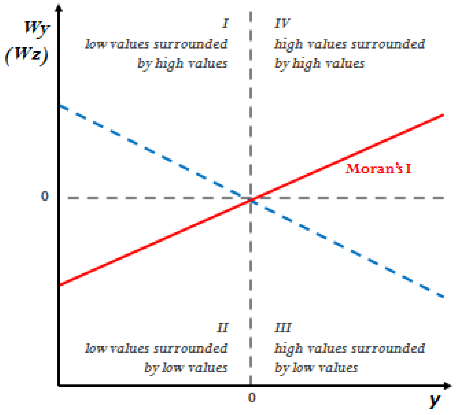
Anselin [27] also provides a graphic representation of the type and value of spatial autocorrelation (the Moran scatter plot) (Figure 1). In the univariate scatter plot, the horizontal axis shows the normalized variable (y), and the normalized ordinate spatial lag of that variable (Wy). In the bivariate scatter plot, a variable on the x axis (y) corresponds to the spatial lag of another variable on the y axis (Wz).

The row passing through the second and fourth quadrants represents positive correlations of values similar to the spatial lag, while the row passing through the first and third quadrants represents a negative correlation of values dissimilar from the spatial lag [17,27,44].

The Moran scatter plot gives no information on the significance of spatial clusters, but it permits the identification of outliers present in the statistical distribution by observing their distance from the row-standardized spatial weights matrix [27]. The significance of the spatial correlation measured through Moran’s I and the Moran scatter plot is highly dependent on the extent of the study area and on the choice of the territorial unit.

The local Moran’s I and its standardized z-score provides an assessment of the similarity of each observation with that of its surroundings [47,48]. For each location, five scenarios emerge:

• Locations with high values of the phenomenon and a high level of similarity with their surroundings (high-high), defined as “hot spots”;
• Locations with low values of the phenomenon and a low level of similarity with their surroundings (low-low), defined as “cold spots”;
• Locations with high values of the phenomenon and a low level of similarity with their surroundings (high-low), defined as “potential spatial outliers”;
• Locations with low values of the phenomenon and a high level of similarity with their surroundings (low-high), defined as “potential spatial outliers”;
• Locations devoid of significant autocorrelations.

3.3. Spatial Regression and Residuals Analysis

A traditional ordinary least squares (OLS) regression was first applied in order to measure the influence of the set of three housing vulnerability indicators on the property listing price variable [30], then spatial autocorrelation tests were performed on the residuals, and finally a spatial LAG regression model was applied to correctly manage the spatial lag dependence.

OLS usually has the following three objectives: to find a good fit between the predicted value (sum of the values of explanatory variables, each multiplied by their regression coefficients), to observe values of the explanatory variable y, and to discover which explanatory variables significantly contribute to the linear relationship.

When dealing with spatial data, it is necessary to test the presence of spatial dependence between the errors or the model variables [49]. Tests for spatial dependence for a single variable are based on the magnitude of an indicator that combines the value observed at each location with the average value at neighboring locations (spatial lags) [17]. Basically, the spatial dependence tests are measures of the similarity between associations in values (covariance, correlation or difference) and associations in space (contiguity) [17]. Spatial autocorrelation is considered to be significant when the spatial autocorrelation statistic takes on an extreme value, compared to what would be expected under the null hypothesis of no spatial autocorrelation.

Spatial effects are tested using the Breusch Pagan test [50] for testing the homogeneity assumption, the Moran test, the Lagrange multiplier (LM) lag test and LM-error tests for testing spatial autocorrelation [49].

When spatial autocorrelation exists, the error term has to take this autocorrelation into account. In this study, a spatial regression model, namely the spatial lag model (SLM) was performed. It takes the following form:

$$y_i={\displaystyle \sum _J}{\alpha }_J{x}_{ij}+\mathsf{\lambda }{\displaystyle \sum _j}{\beta }_j{z}_{ij}+{\epsilon }_i$$

(4)

where $\lambda$ is the spatially observed value lag coefficient, and $u_i$ is the random error for location i.

When significant spatial autocorrelation exists either globally or locally, spatial heterogeneity exists [17,47].

4. Case Study

The city of Turin is assumed as an emblematic case study of former-industrial cities since, as with other similar European cities, it has suffered deep social and economic transformations in terms of its potential for new redevelopment.

The city of Turin covers an area of 130.17 square kilometers, has 883,281 inhabitants [51], and the population density of the city, equal to 6.846 ab/sq·km, varies greatly over the different territorial segments. The city is divided into the following main urban areas: the historical city center with a high presence of historical buildings; the hillside on the right side of the river Po, with a high presence of high-income population and villas with gardens; the first expansion area, which hosts middle-class level buildings; and the suburbs, mainly built in the 1960s, where most of the industrial buildings (now mainly abandoned) are located. In agreement with [52,53], this classification of the city also represents the broad division of real estate sub-markets whose trends perfectly reflect the increasing gap between upper classes and the low-income population. Over 16.5% of the urban territory is occupied by 21 square kilometers of green areas, and 44% of that is comprised of historical gardens [54].

In total, 56.71% of the building stock is residential, 5.20% is industrial buildings and 1.76% is unused space. The residential real estate market of the city is monitored and analyzed by the Turin Real Estate Market Observatory (TREMO) [55], which was founded in 2000 [56]. The sample used in this study belongs to a database property of TREMO, which included, among others, property prices and the buildings’ quality characteristics. It consisted of 3071 property listings in Turin published in 2011–2017 on one of the main Italian real estate advertisement websites. The dataset was selected from a database of 3381 items, from which the outliers and the observations with missing addresses were eliminated.

The data related to the buildings’ construction period and condition derive from the data warehouse of the 15th population and housing census, implemented in 2011 by the Italian National Institute of Statistics (ISTAT) [57]. ISTAT is a public research organization; it has been present in Italy since 1926 and is the main producer of official statistics. It operates in complete independence and with continuous interaction with the academic and scientific communities [58]. The census contains a wealth of information, at a sub-municipal level (3852 census cells), about the demographic and social structure of the population resident in Turin and in the related housing stock.

In the last few years, some studies were carried out in order to study the market and territorial segmentation of the city of Turin [10,35,36,38]. One of the most important segmentations of Turin is based on the 40 microzones (submarkets), defined in 1999 by Politecnico di Torino and approved by the Municipal Council in accordance with DPR 138/98 and the Regulation issued by the Ministry of Finance. A series of studies on the city of Turin analyzed the relation between property prices and microzones [35,36], as well as other different territorial segmentations, such as the 3852 census cells and the 93 historical territorial units based on an urban and historical analysis developed in 2011 by Politecnico di Torino [10,38]. Microzones currently need to be updated in order to take into consideration the most recent transformations that have occurred at the urban level; therefore, with this aim, in this study, a smaller administrative urban segmentation was selected: the 94 statistical zones (SZ), defined by ISTAT as aggregations of census cells.

5. Results

The three-step methodology outlined in Section 3 was applied with a twofold purpose. Firstly, the final set of housing vulnerability indicators (BEC, BMB and B4670) was analyzed in order to investigate their relation with the property prices by means of spatial analyses. Secondly, the two housing vulnerability indicators that significantly influenced the real estate market were compared to two social vulnerability indicators that a previous study highlighted as having a significant explanatory power in the property price determination process. In this comparison, the spatial analyses were performed to stress some similarities among the two dimensions of housing and social vulnerability.

5.1. Housing Vulnerability and the Real Estate Market

5.1.1. Selection of Housing Vulnerability Indicators and Property Prices Analysis

To analyze the variability of the most vulnerable housing stock features in relation with the real estate market, an initial set of variables was selected with reference to the buildings’ construction period, building condition and building quality (

Table 1. Descriptive statistics of the initial set of characteristics selected (Source: Authors’ elaboration on Italian National Institute of Statistics (ISTAT) and Turin Real Estate Market Observatory (TREMO) data).

Variable	Variable Description	Data Source	Percentage (%)
B < 19	Buildings built in the time period <1919	ISTAT	14%
B19–45	Buildings built in the time period <1919–1945	ISTAT	21%
B46–60	Buildings built in the time period 1946–1960	ISTAT	28%
B61–70	Buildings built in the time period 1961–1970	ISTAT	21%
B71–80	Buildings built in the time period 1971–1980	ISTAT	9%
B81–90	Buildings built in the time period 1981–1990	ISTAT	3%
B91–00	Buildings built in the time period 1991–2000	ISTAT	2%
B01–05	Buildings built in the time period 2001–2005	ISTAT	1%
B > 05	Buildings built in the time period >2005	ISTAT	1%
BGood	Buildings with a good state of conservation	ISTAT	26%
BAver	Buildings with an average state of conservation	ISTAT	62%
BMed	Buildings with a mediocre state of conservation	ISTAT	11%
BBad	Buildings with a bad state of conservation	ISTAT	1%
BClas	Classy buildings	TREMO	7%
BDist	Distinguished buildings	TREMO	22%
BMLev	Medium-level buildings	TREMO	41%
BEco	Economical buildings	TREMO	27%
BCouncil	Council houses	TREMO	3%

).

As shown in Table 1, in the city of Turin, 49% of the building stock is built between 1946 and 1970. The residential building stock is mainly in an average state of conservation (62%), and the building quality is classified at a medium level (41%).

Therefore, as highlighted in Section 3, a set of three housing vulnerability indicators was developed and a geographical database was built that also included property prices (

Table 2. Descriptive statistics of the selected indicators across the 94 statistical zones (SZ) (Source: Authors’ elaboration on ISTAT and TREMO data).

Variable		Data Source	Mean (€/m2)	St. Dev (€/m2)
LP	Property Listing Price mean	TREMO	2402.02	1064.517
Indicators		Data Source	Mean	St. Dev
B4670	Buildings built in the time period 1946–1970	ISTAT	0.441	0.185
BMB	Buildings with a bad/mediocre state of conservation	ISTAT	0.107	0.078
BEC	Economical buildings and council houses	TREMO	0.309	0.253

).

The variation across the 94 SZ is detailed as follows: B4670 ranged from 0.041 to 0.909, with an average score of 0.441; the BMB ranged from 0.005 to 0.422, with an average score of 0.107; the BEC ranged from 0.000 to 1, with an average score of 0.309.

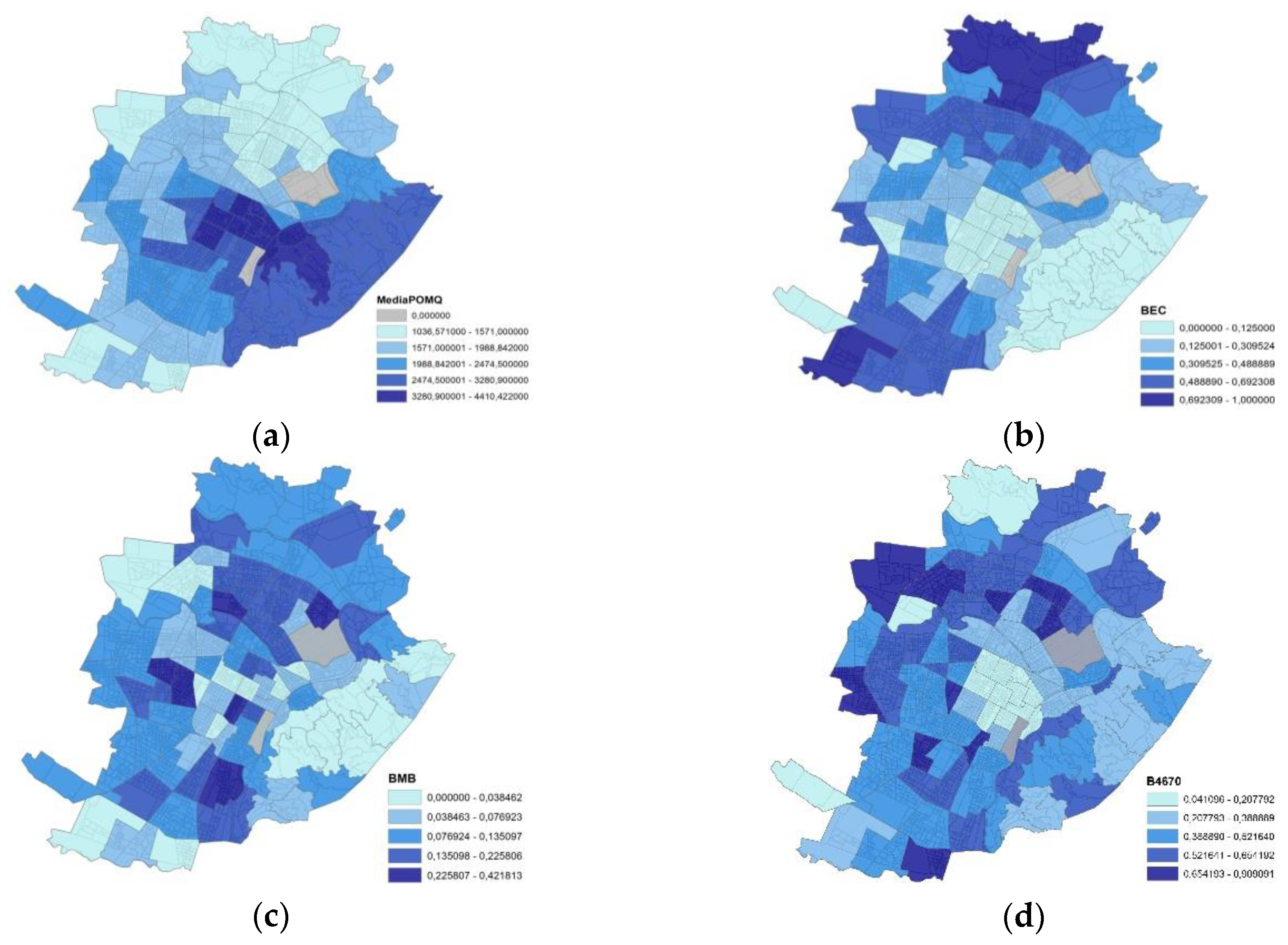
Figure 2 shows how the three indicators and the property price variable (LP) are distributed into the 94 SZ.

In Figure 2a, four distinct price ranges clearly identify four defined areas of the city. The most expensive building stock is in the city center and on the hillside, while medium price buildings are located in the first ring area around the historical center and those with the lowest prices are located in the north and south areas. As we can see, there are some infrastructure axes that appear to represent ideal borders. For example, the course axis Regina Margherita is, rather clearly, a division between the central most wealthy areas and the poorest ones; at the same time, however, we note the presence of low price areas also in the south of via Onorato Vigliani [59]. The pattern of BEC in Figure 2b suggested a correlation between BEC and LP.

The pattern of B4670 (d) highlighted a quite extended area of the hill characterized by a low presence of buildings built during the time period 1946–1970; otherwise, the BMB indicator (c) seems to be quite randomly distributed in the city segmentation.

5.1.2. Preliminary Correlation and Exploratory Spatial Data Analyses (ESDA)

Spatial analyses were performed to focus on the spatial components of the housing vulnerability indicators and property prices.

Initially, the three housing vulnerability indicators (BEC, BMB and B4670) were taken into account and their correlation with the LP variable was tested by means of a Spearman correlation test. Results showed a high negative correlation between all the indicators and LP and highlighted BEC as the indicator that was most negatively correlated with the LP variable. The correlation between the indicators themselves was also verified before applying a regression model (

Table 3. Spearman correlation test (Source: Authors’ elaboration).

Variable	LP	BEC	BMB	B4670
LP	1	−0.645	−0.266	−0.484
BEC	−0.645	1	0.285	0.391
BMB	−0.266	0.285	1	−0.001
B4670	−0.484	0.391	−0.001	1

).

Subsequently, spatial autocorrelation was calculated to measure the local spatial association level between each territorial unit and the neighboring units. In particular, to consider the dimension of geo-spatial clustering of property prices and housing vulnerability indicators, the Moran’s I statistics for each variable and LISA were calculated and the spatial relationship between the 94 SZ was examined. A significance calculation (99 permutation) processed by GeoDa on the basis of Monte Carlo statistics confirmed the significance of the clusters, with a p-value of between 0.001 and 0.05 [60].

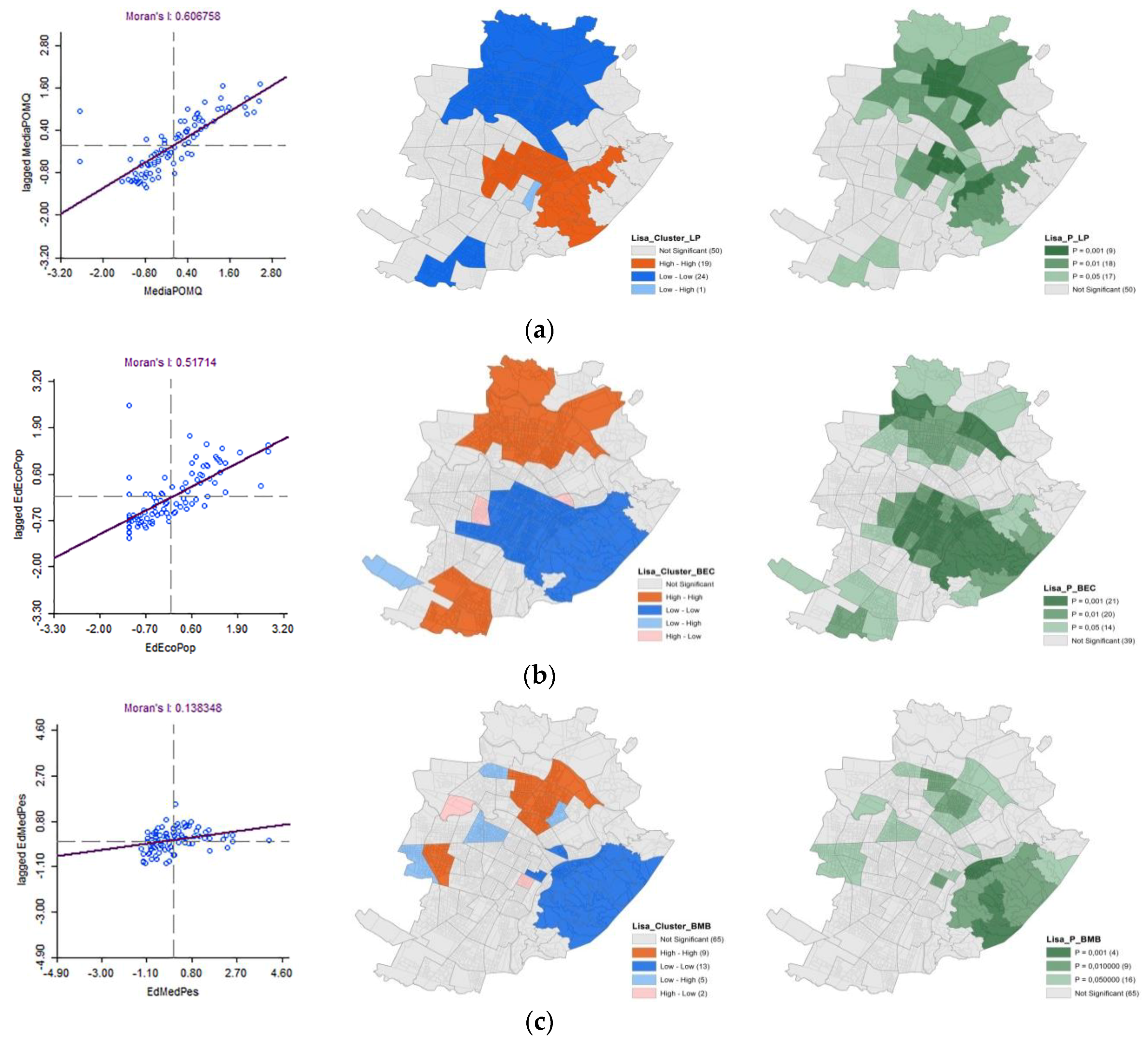
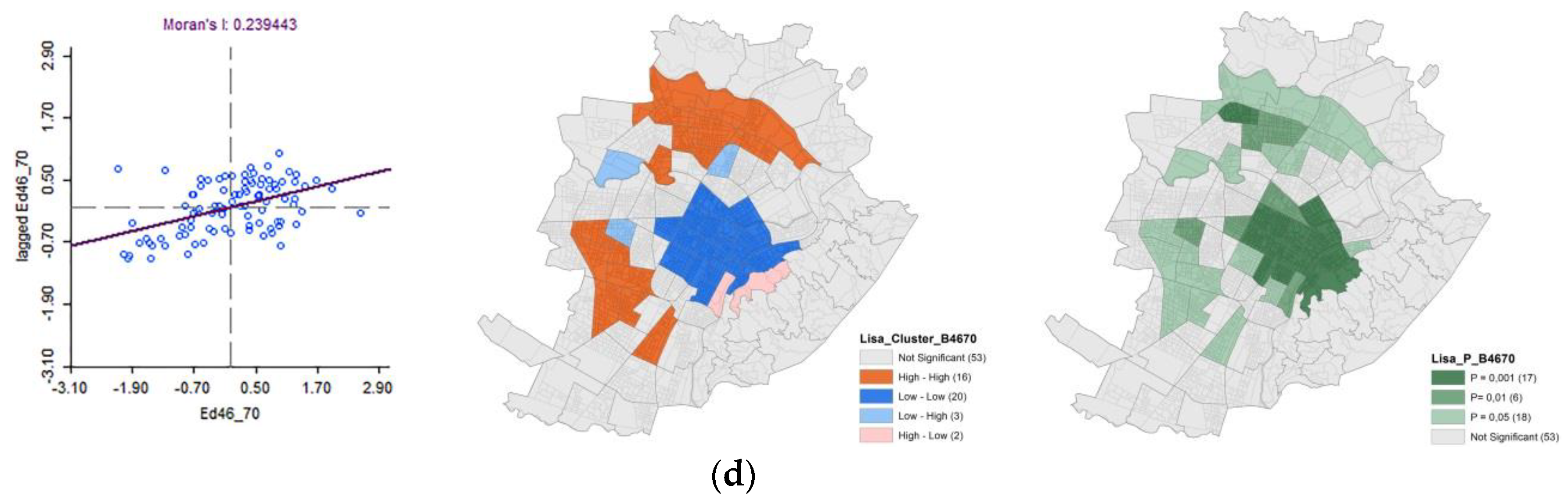
Figure 3 shows the results of Moran’s Index and LISA clustering for LP and the three housing vulnerability indicators.

By means of the Moran scatter plot, the presence of a positive autocorrelation across the SZ was verified since most of the observations were located in the II and IV quadrants. There were also some hypothetical outliers with data that were distant from the mean. Furthermore, findings suggested geo-spatial clustering in all the variables, and the highest value of autocorrelation was observed for the LP variable (Moran’s I = 0.609), followed by BEC (Moran’s I = 0.517).

LISA analysis identified spatial clusters that represented the highest concentration of the most and least vulnerable housing stock. The LISA results suggested striking geographic clustering of property prices in the central, northern and southern urban areas (a). A first cluster, located in the north and in the south areas of the city, represented the urban areas characterized by a positive autocorrelation of high values and a high level of similarity with their surroundings (high–high). A second cluster, located in the city center and on the hills, represented the urban areas characterized by the positive autocorrelation of low values and a low level of similarity with their surroundings (low–low).

A similar clustering was observed in the case of the economical buildings and council houses (BEC) (b): in particular, it is possible to notice a certain reverse correspondence between the spatial clusters obtained for property prices and those obtained with BEC: the BEC high–high LISA cluster corresponds to the LP low–low LISA cluster, and vice versa.

The results presented in Figure 3 provide compelling evidence that the urban areas characterized by the presence of economical buildings and council houses were also more likely to record low price housing rates. Furthermore, the SZ located on the hills is characterized by a low presence of buildings with a bad/mediocre state of conservation (c), while the central part of the city is characterized by a low concentration of buildings built during the Post-World War II period, identified by a smaller cluster of SZ between the “Aurora” district and “Vittorio Veneto” square (d).

5.1.3. Spatial Regression and Residuals Analysis

The spatial lag model outlined in the methodology section was applied to assess the influence of housing vulnerability indicators on property prices. The dependent variable is LP, while the independent variables are BEC, BMB and B4670.

Since we found considerable geo-spatial clustering in the dependent and explanatory variables, we presented the results of both the OLS model and Spatial Lag model (

Table 4. Ordinary least squares (OLS) model and Lagrange multiplier (LM) spatial lag model to assess the relation between LP, BEC, BMB and B4670 (Source: Authors’ elaboration).

Variable	OLS Model for Housing Vulnerability		LM Spatial Lag Model for Housing Vulnerability
	Coefficients	Probability	Coefficients	Probability
Spatial coefficient (W)			0.614	0.000
BEC	−1683	0.000	−722	0.006
BMB	−1383	0.116	−440	0.537
B4670	−1351	0.001	−940	0.003
Constant	3545	0.000	1572	0.000
Number of observations	94		94
Log likelihood	−736.3		−722.5
AIC	1480.6		1455.02
R square	0.493		0.653
Breush–Pagan test for diagnosing heteroskedasticity	26.205	0.000	33.305	0.000
Likelihood ratio test			27.580	0.000

).

The results of the spatial lag model account for the geo-spatial variable (W) in the dependent and explanatory variables. The findings revealed the improvement of the model with the introduction of the spatial variable (W) with an R-squared rising from 0.49 to 0.65. The findings also suggested that the presence of economical buildings and council houses (BEC) and buildings built during the time period 1946–1970 (B4670) had a significant and negative influence on them.

Furthermore, a residuals analysis illustrates that the spatial pattern is almost certainly the main factor that causes the variables autocorrelation. This is evident by comparing the OLS residuals Moran scatter plot (Figure 4a) with the LAG residuals one (Figure 4b).

5.2. Comparison between Housing and Social Vulnerability Indicators

The results of the spatial analyses on the three housing vulnerability indicators highlighted that only two of them (BEC and B4670) had a significant and negative influence on property prices. Therefore, the final step of this research is aimed at comparing these two housing vulnerability indicators with the following two social vulnerability indicators, based on ISTAT data, that a previous study [10] highlighted as having a significant and negative explanatory power in the property price determination process:

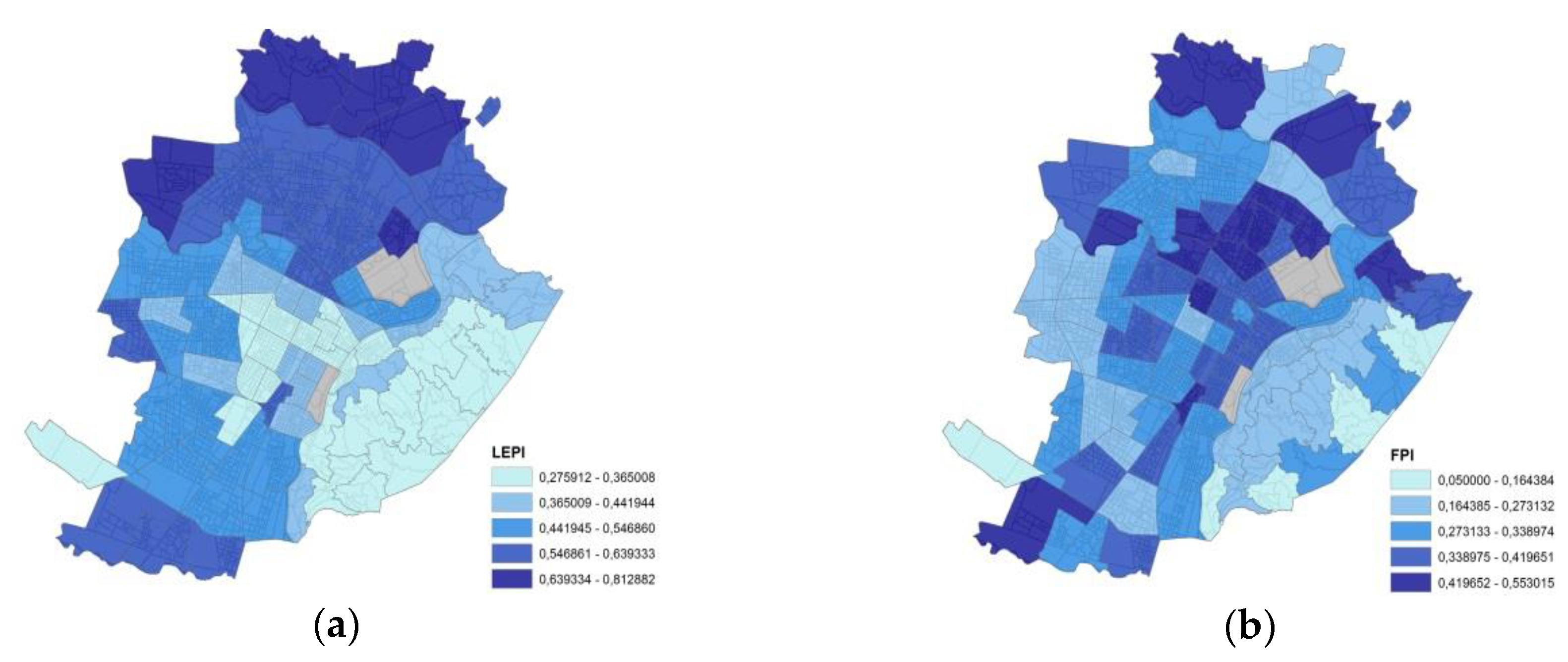
• the low education population indicator (LEPI), which represents the percentage of literate and illiterate inhabitants and people with a primary/middle school certificate;
• the foreign population indicator (FPI), which represents the percentage of foreigners from Africa and America living in Italy.

Figure 5 shows the spatial distribution of LEPI (a) and FPI (b) in the 94 SZ: LEPI ranged from 0.276 to 0.813, with an average score of 0.47, while FPI ranged from 0.05 to 0.553, with an average score of 0.323.

5.2.1. Preliminary Correlation and Exploratory Spatial Data Analyses (ESDA)

The Spearman correlation test showed a high negative correlation both between BEC and LP −0.65) and between LEPI and LP (−0.76). Moreover, it showed a high and positive correlation between BEC and LEPI (0.84) (

Table 5. Spearman correlation test (Source: Authors’ elaboration).

Variable	LP	BEC	B4670	FPI	LEPI
LP	1	−0.645	−0.484	−0.250	−0.764
BEC	−0.645	1	0.391	0.332	0.840
B4670	−0.484	0.391	1	0.003	0.417
FPI	−0.250	0.332	0.003	1	0.493
LEPI	−0.764	0.840	0.417	0.493	1

).

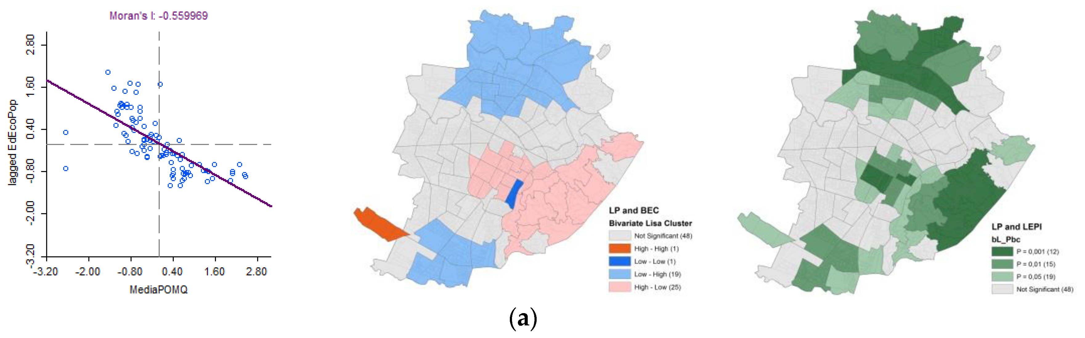
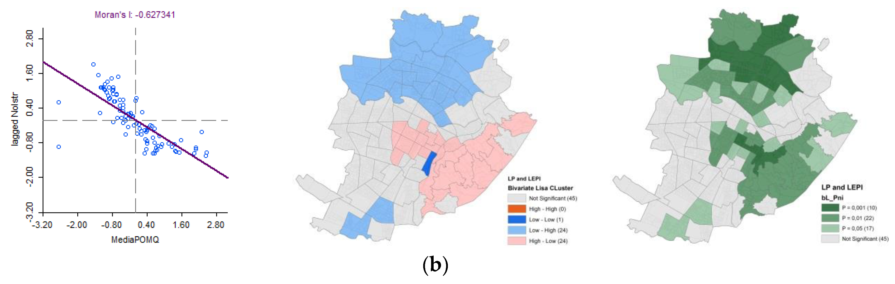
Table 5 also shows that FPI seemed not to be highly correlated either with LP or with other indicators. The high positive correlation between BEC and LEPI suggested different interpretations that could be confirmed also by the spatial dependence analysis performed by means of a bivariate local Moran’s statistic (Figure 6).

Both bivariate Moran scatter plots highlighted a negative correlation between BEC/LEPI and the spatial lag of LP. The inverse correspondence between LP/BEC and LP/LEPI is also shown in the maps with high–low and low–high clusters.

5.2.2. Spatial Regression and Residuals Analysis

Assuming the high correlation between BEC and LEPI and their noteworthy similarity in the spatial clustering, the last step of the methodology was applied by replacing BEC with LEPI as an explanatory variable of the OLS and Spatial Lag regression models previously performed (Table 4).

The results in

Table 6. OLS model and LM spatial lag model to assess the association between LP, LEPI, BMB and B4640 (Source: Authors’ elaboration).

Variable	OLS Model for Housing Vulnerability		LM Spatial Lag Model for Housing Vulnerability
	Coefficients	Probability	Coefficients	Probability
Spatial coefficient (W)			0.452	0.000
LEPI	−4672	0.000	−2847	0.000
BMB	−312	0.692	12.606	0.986
B4670	−956	0.006	−779	0.011
Constant	4942	0.000	2940	0.000
Number of observations	94		94
Log likelihood	−723.159		−716.5
AIC	1454.32		1443.11
R square	0.617		0.681
Breush–Pagan test for diagnosing heteroskedasticity	37.575	0.000	41.239	0.000
Likelihood ratio test			13.207	0.000

confirmed that LEPI had a significant and negative influence on property prices which was higher than BEC. Comparing the results in Table 4 and Table 6, it is possible to notice that the two spatial LAG regression models have a quite comparable prediction power.

Furthermore, the residuals analysis results highlighted that, also in this case, the spatial pattern is almost certainly the main factor behind the variables autocorrelation since the residual spatial correlation disappears when using a spatial LAG model (Figure 7b), instead of a OLS model (Figure 7a).

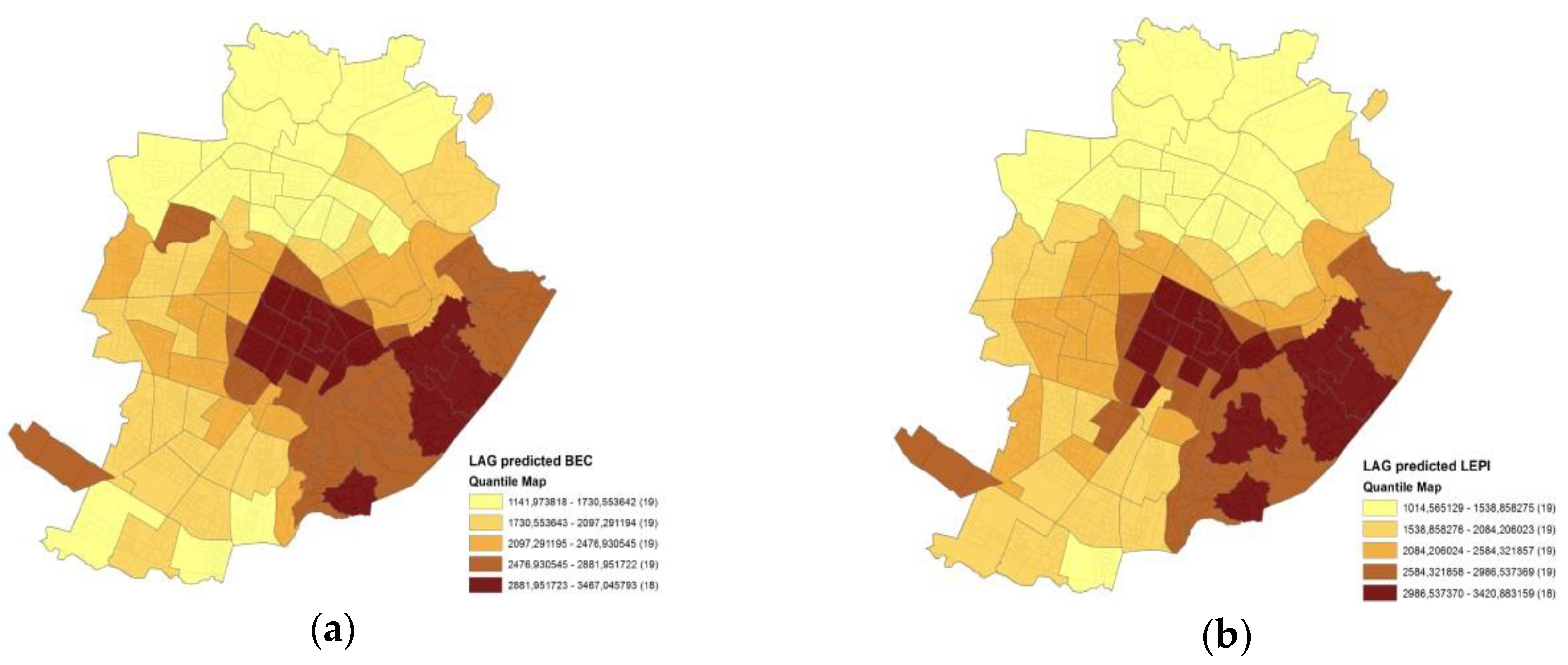
Finally, the comparison of the predicted values of the two spatial LAG models, represented by means of quantile maps in Figure 8, highlights two very similar patterns.

It is evident that in both maps there are clusters of higher values (brown-colored) in the city center and on the hillside, while in the northern part of the city there is a bigger cluster of lower values (yellow colored). Therefore, by finally comparing these patterns with the natural breaks map of the property prices (Figure 2a), it is possible to acknowledge a high similarity and conclude that both spatial LAG regression models have a good fit with reality and a quite comparable prediction power.

6. Conclusions

In the broader framework of research aimed at the vulnerability and resilience of cities and territories, in this paper, a three-step methodology is proposed to specifically analyze housing vulnerability and its relation with the real estate market. The first step of the methodology, by means of studying an initial set of buildings’ physical features, developed a set of three housing vulnerability indicators: buildings built between 1946 and 1970 (B4670); economical buildings and council houses (BEC); and buildings in a mediocre or bad state of conservation (BMB). The value for each indicator and the property prices, calculated for each territorial unit, constituted the geographical database to be analyzed assuming the case of Turin and its administrative spatial segmentation in 94 statistical zones. The second step, based on correlation analysis and exploratory spatial data analyses (ESDA), highlighted a high negative correlation between the property prices and all the indicators, with particular reference to BEC. Furthermore, the outcomes showed the highest value of spatial autocorrelation for BEC and a certain reverse correspondence between the spatial clusters obtained for property prices and those obtained with BEC.

The results of a spatial LAG regression model, applied as the third step of the methodology, highlighted that only two indicators (BEC and B4670) had a significant and negative influence on property prices. Furthermore, the residuals analysis revealed that the spatial pattern was almost certainly the main factor that caused the variables’ autocorrelation since the residual spatial correlation disappeared using the spatial LAG model.

Subsequently, the analysis of the housing vulnerability indicators was extended in order to compare them with two social vulnerability indicators that a previous study [10] highlighted as having a significant and negative explanatory power in the property price determination process: the low education population indicator (LEPI) and the foreign population indicator (FPI). This comparison mainly showed a high and positive correlation between BEC and LEPI, a significant and negative influence on property prices for both indicators (even if higher for LEPI) and a noteworthy similarity in the spatial clustering. This similarity was also confirmed by the comparison of the spatial distribution of the predicted values of two spatial LAG models, performed by using BEC as an explanatory variable in the first case and by using LEPI in the second case. The quantile maps indeed highlighted two very similar patterns, in line also with the spatial distribution of the property prices; this means that both of the performed spatial LAG regression models have a good fit with reality and a quite comparable prediction power.

Therefore, it is possible to conclude that a spatial correlation between housing vulnerability, social vulnerability and the real estate market exists, and so the relation between buildings’ physical features, fragile sectors of the population and property price variability deserves to be investigated and spatially analyzed in order to correctly measure the vulnerability of cities and territories.

Furthermore, with particular reference to the context of the city of Turin, it is possible to highlight other more specific outcomes.

The results of this study allow us to spatially identify and analyze the most vulnerable areas of the city, characterized by the presence of buildings built between 1946 and 1970, which represent a great part (49%) of the building stock. Currently, these buildings, which present low-quality materials, high energy requirements and obsolete systems inadequate to guarantee the required “comfort” levels, are mostly energy inefficient and need to be renovated. Moreover, they are located in suburbs that are characterized by low property prices and are inhabited by a low-income population. For these reasons, the convenience and the feasibility of the restructuring works are uncertain since these are too expensive in comparison with the property prices of these sub-markets and owners cannot afford it, even if energy retrofit policies are promoted both at the national and municipal level. In addition, as is usually the case in Italy in these kinds of context, it is difficult to proceed to real interventions since there are numerous residential units, each with a different owner with a different willingness to pay.

With regard to the spatial correlation clusters, they effectively correspond not only to the most and the least vulnerable housing stock but also to the most and the least vulnerable social classes of population. Indeed, the results of this study allow us not only to identify the clusters of urban areas characterized by the most vulnerable built environments, the most vulnerable sectors of the population and the lowest property prices, but also the “opposite” clusters. These identify the central area and the hillside, where historically the architecture typologies and locations represent the social upper classes of the inhabitants well. The second “indirect” result is the definition of a “grey” area of the city, where the presence or absence of housing vulnerability is not clustered, but randomized. These areas, which are characterized by medium level quality buildings, inhabited by the middle classes of the population, need to be more deeply analyzed. The presence of huge inequalities at the urban level related to the social condition of the population is evident from our spatial analyses and it is perfectly reflected by the spatial distribution of property prices, even if it deserves to be further explored.

Future studies can be addressed in different directions. First of all, the research could be focused on further exploring social and housing vulnerability indicators in other cities for comparison with the city of Turin. Secondly, on the basis of the availability of additional data (from different sources), the research can be developed by providing other indicators related to other issues and by studying the relations between them in order to support the construction of vulnerability/resilience indexes. These analyses could lead to the territorial administrative segmentations of the urban areas being updated and the definition of parcels of different dimension (smaller and bigger) which are able to better explain different territorial and socio-economic dynamics. For example, it will be possible to analyze the infrastructure net, with its positive (easy access) or negative (noise/pollution) influence on the real estate market. The study of housing and social vulnerability could also be useful for the review process of the current city plan of Turin in order to identify the most vulnerable urban areas and to support strategic redevelopment policies. The Municipality of Turin should also promote specific policies in order to compensate the inequalities of these urban areas by encouraging new public and private investment. For example, a series of supporting actions could be further implemented, such us the tax exemption for energy retrofit interventions, the granting of additional building surfaces for those who implement energy saving improvements, the enhancement of public spaces and the placement of new public services. In doing this, the municipal policies can be effectively oriented in order to redevelop the most vulnerable urban areas, fostering an integrated social and territorial welfare.

Limitations of the Study

One of the key limitations of this study was the non-availability of transaction prices due to the lack of public data in the Italian context; therefore, we had to use a sample of listing prices as a proxy of the actual transaction prices, as justified by the literature.

Moreover, another key limitation of the analysis was the limited availability of housing data at the census cell level. The lack of transparency and distribution of open data at a fine scale limited the analysis on the selected buildings’ features, excluding some other interesting potential variables.