Modeling a Three-Mode Hybrid Port-Hinterland Freight Intermodal Distribution Network with Environmental Consideration: The Case of the Yangtze River Economic Belt in China

Abstract

Efficiency challenges of the hinterland connectivity, along with growing green concerns necessitate the integration of economic goals and environmental considerations, for port-hinterland logistics problems. This study focused on innovative modeling, for a three-mode port-hinterland intermodal freight distribution system, from the perspective of shippers. A hybrid distribution network topology, combining point to point, hub-and-spoke, and connected hubs was designed as route alternatives for loads from origin to destination. A bi-objective decision framework involving analytical scenarios of emissions limitation, emissions taxation, and an emissions trading scheme, was developed for policy analysis, and then applied to a real-life hinterland logistics network in the Yangtze River Economic Belt in China. The results showed that the implementation of the three emissions policies, all resulted in great changes in flows between intermodal routes and achieved emissions reduction goals. Nevertheless, the conflict between logistics costs and carbon emissions, differs from policy to policy. Some inflection points were identified to offer decision supports on policy insights, for the port-hinterland distribution network. Lastly, a sensitivity analysis on cost and emissions parameters was given. It revealed that the flow changes and trade-off relationship between economic and environmental objectives, were both sensitive to the road transportation mode.

1. Introduction

Increasing international container volume worldwide, due to the intensification of global trade is creating pressures not only on maritime shipping, but also on the port-hinterland connections, which stimulates shippers to develop competitive container supply chains to move cargoes more efficiently [1,2,3]. Port-hinterland interaction, as one of the significant components in achieving efficient global logistics chains, is adapting to the trend where competition between supply chains is more emphasized than port competition between port authorities, shippers, and carriers [4]. Although containerization and the emerging maritime shipping network have helped the maritime logistics services of global supply chains to become very efficient, the efficiency of the hinterland logistics system, which connects manufacturing and consumption regions to the maritime shipping part still faces challenges. In this context, intermodal transportation emerges and has developed as a significant choice to compete with road transportation in the movement of cargoes in hinterlands [5,6,7]. Significant attention on intermodal transport is given to railway-road transport [8,9,10], whilst few studies talk about the waterway-road intermodal option [11,12]. This may be explained by geographical reasons. Most countries may have access to rail, but it may not get to the barge. Specifically, there are a small number of countries where both inland rail and barge transport can be employed by transport users. For instance, in China, both the inland railway network and the main waterway system along the Yangtze River have the accessibility of freight transport services. This situation allows the possibility of various intermodal transportation forms including road-rail, road-barge, rail-barge, and barge-rail, etc.

The design of an intermodal transportation network, is one of the most important decisions in intermodal logistics planning [10,13]. Hub location theory is mostly used in the model, where the total costs of the freight network are minimized under some assumptions and constraints. Arnold et al. [14] addressed the problem of optimally locating rail/road terminals for freight transport, and developed five planning scenarios. Racunica and Wynter [15] developed an optimization model to address the problem of increasing the share of rail in intermodal transport, through the use of hub-and-spoke type networks for freight rail. Limbourg and Jourquin [16] proposed an iterative procedure based on both the p-hub median problem and the multi-modal assignment problem, for the European rail/road network. These studies developed inter modal transport planning models by investigating the combination of road transport with another mode, i.e., railway or waterway. However, the integration of road, railway, and waterway modes simultaneously, is rarely studied. Macharis et al. [17] developed a LAMBIT model which incorporated various network layers of transportation modes of road, rail, and inland waterways for evaluating fuel price increase on the market area of intermodal transport. Zhang et al. [18] developed a freight transport optimization model incorporating multimodal infrastructure; hub-based service network structures with inclusion of road, rail, and inland waterways; and various design objectives of multiple actors. Although these studies considered three transportation modes, they only talked about the intermodal transportation forms of road-rail and road-waterway, simultaneously. They did not consider the possibility of more complex intermodal forms in some hinterland regions, where river systems and freight rail systems are both available. Thus, this paper intends to investigate the innovative design of intermodal logistics systems in hinterlands involving more complex intermodal transportation combinations.

Environmental protection is a popular issue worldwide, and the mitigation of greenhouse gases (GHG) in the logistics and transportation industries has absorbed the attention of both government and academia over the years [19]. The transportation sector is the second largest source of global CO₂ emissions, with the share of 24%, where road transport accounts for three quarters of the total emissions [20]. In response to the increasing emissions by road transport, low-carbon transportation modes, including rail and river shipping, have been encouraged in Europe for long-distance travel [21]. In other words, in addition to the cost-saving goal, the objective of reducing CO₂ emissions has been considered in logistics planning problems. Consequently, a wide range of research on green logistics [22,23] and green supply chain management [24,25], have been published in the past two decades. Conventional logistics planning problems in intermodal freight transportation, mainly focus on a pure cost minimization model [5,26,27]. Within creasing concerns on issues of environmental protection, there exist some models targeting carbon emissions minimization [28,29]. Additionally, there are growing research papers discussing economic and environmental objectives, simultaneously, in the modeling [24,30]. One research direction focuses on the trade-off analysis between economic and environmental goals [31,32,33]. The other promising direction prefers to employ the approach of internalizing carbon emissions effects through market-based instruments, namely taxes, charges, or Emissions Trading Schemes (ETS) [34]. For instance, Fahimnia et al. [35] investigated the potential impacts of carbon tax policy, on the financial and emissions reduction of supply chains, through developing a planning model that integrated economic objectives and CO₂ emissions goals at the tactical planning level. Zhang et al. [18] proposed a freight transport optimization model incorporating terminal network configuration, hub-based network design, and carbon pricing policy simultaneously, and they calibrated and validated it by using real data from a hinterland container transport network in the Netherlands. As for Emissions Trading Schemes, it is mainly explored and studied in the aviation industry or shipping sector in the transportation field. Vespermann and Wald [36] explored the economic and ecological impacts that were caused by an inclusion of the aviation industry into the EU-ETS system, and a simulation model was employed. Wang et al. [37] investigated the economic implications of open ETS and Maritime ETS mechanisms, on the container shipping sector and the dry bulk shipping sector.

Nevertheless, an integrated decision framework that addresses multi-objective optimization problems by employing various environmental policy interventions has been rarely analyzed. The purpose of this study was to provide a comprehensive decision framework, for a port-hinterland distribution network in which road, railway, and inland waterways are all encompassed; by including both trade-off analysis and environmental policy intervention analysis. Such a decision framework could help offer comprehensive insights for shippers on the strategic decisions about transportation mode selection, intermodal terminal choice, and flows distribution, under various emissions control policies. Therefore, this study will break away from the literature by building a bi-objective model, for a three-mode hybrid port-hinterland intermodal distribution network. Minimizations of logistics costs and CO₂ emissions generation, are two major decision objectives. Three analytical scenarios, including emissions limitation, emissions taxation policy, and emissions trading schemes were analyzed; supporting policy analysis.

Moreover, there are two additional gaps in the implementation of emissions trading schemes in the port-hinterland logistics network. One is that ETS is mainly used in the aviation or shipping sectors and is rarely studied, for hinterland intermodal logistics systems. The other is about questions of how emissions permits are allocated, and what permit trading price can be accepted. The existing research usually discusses ETS under the assumption that the number of located permits (or the cap) for firms is fixed, or the trading price is set as one fixed value (i.e., the actual prices in those countries where ETS has been implemented in practice). This study plans to discuss ETS application by considering, both the number of permits located and permit trading price, as decisions in the modeling. Therefore, this paper will fill these gaps.

The remainder of this paper is organized as follows. The modeling approach, analysis framework, case description, and data source are provided in Section 2. Section 3 presents the results of the proposed model, as applied in the port-hinterland distribution network of the Yangtze River Economic Belt in China. Section 4 gives an extended discussion of findings. Finally, the conclusions and further research directions are discussed in Section 5.

2. Materials and Methods

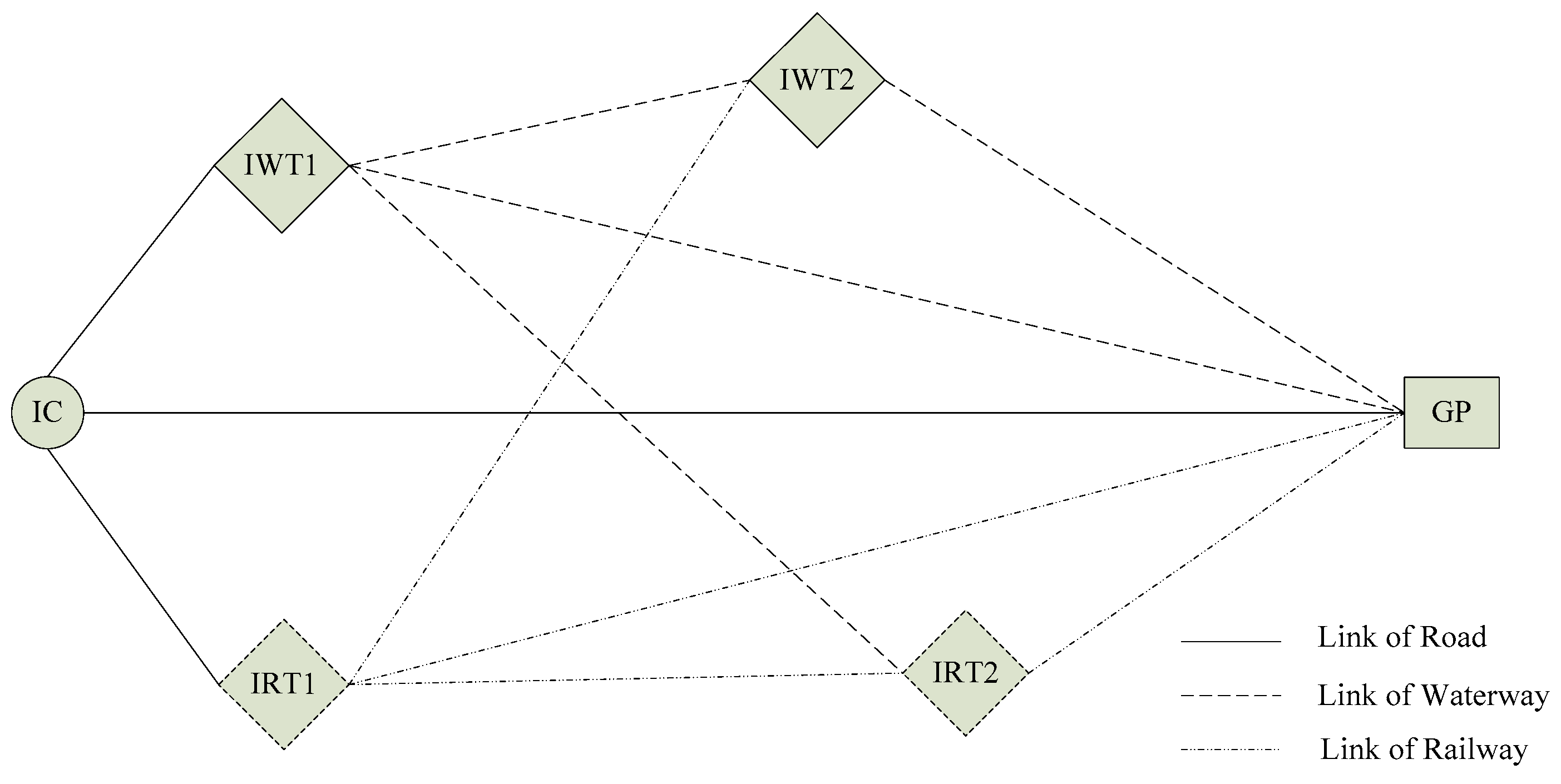
The modeling approach was based on a generic port-hinterland distribution network problem, which consists of a lot of nodes of inland cities (IC), inland waterway terminals (IWT), inland railway terminals (IRT), gateway seaports (GP), and transport links of road, waterway, and railway. Various network designs have been applied in intermodal freight transportation, including options of direct links, corridor, hub-and-spoke, connected hubs, static routes, and dynamic routes [10]. This study presented a hybrid network topology, which involved direct point-to-point link, hub-and-spoke, and connected hubs designs as alternatives for logistics chains selection. Therefore, the problem was not a standard hub-spoke network problem, but one in which freight in inland cities could be transported to seaport destinations through the direct road links, visiting only one inland intermodal terminal (IIT), also routing through multiple terminals (hubs) of the same type or different type; but at most two connected terminals designed in a whole chain. On top of that, an inland city node could be assigned to more than one IIT, under certain capacity restrictions.

The detailed network illustration is presented in Figure 1. Containerized goods that are generated at the origins of inland cities, need to be transported to the destinations of gateway seaports through the proposed inland distribution network. There are three transportation modes of road, waterway, and railway available. Containers will be transported to seaports all the way by truck, if there is no container barge port or rail station nearby. Alternatively, if an IWT or IRT is available, they can be transshipped, for one or at most two times. In this way, containers are collected by truck before they are consolidated at the first assigned terminal, and then they wait for the main waterway transport or railway or inter-terminal transshipment. As for the inter-terminal design, two common forms are IWT-IWT and IRT-IRT transshipment [33], in which the goods are transshipped twice by waterway or railway, for the main haul of intermodal transport. However, some special intermodal transport forms, which refer to the connections between terminals of different types, namely IWT-IRT or IRT-IWT, will be designed and included in this paper. These forms come up with the possibility that there exist a few inland cities, which are equipped with both infrastructures of container ports and railway stations. It means goods can be transferred between barge and rail. Thus, the distribution network designed in this study can better reflect the reality of the hinterland logistics system, especially in countries where the inland waterway system requires integration with the railway system.

2.1. A Bi-Objective Model Formulation

Economic and environmental aspects were integrated, through a bi-objective modeling approach. The two objectives of the model were logistics costs minimization and greenhouse gas emissions minimization, through the port-hinterland distribution network, given freight transport demand and some capacity restrictions. The freight loading unit in this study was assumed to be a container (measured in TEU). Transportation costs, were the sum of the costs of transportation links and container handling costs at IITs. Transit time included link-related transportation time, and terminal-related handling and storage time. Environment-related greenhouse gas emissions were represented by the CO₂ emissions generation, which consisted of emissions produced in transportation activities, as well as those released in the handling process at IITs. Since the focus of this study was on the confliction between cost objectives and carbon emissions objectives, the aspect of time performance was converted into time cost and added to logistics costs in modeling. Container transport demands of inland cities were assumed to be fixed. In real life, inland intermodal terminal and gateway seaports, have the maximum capacity for handling containers. Therefore, several container capacity restrictions on all inland intermodal terminals and gateway seaports were attached in this paper, to better reflect reality. The choices of transport routes, flow distribution, and gateway ports were determined by the competition in total logistics costs or total carbon emissions.

2.1.1. Formulation

Transportation Costs through the Port-Hinterland Distribution Network

Transportation costs are formulated as seen in Equation (1). The first composition, are the sum of the direct transportation costs from inland cities to gateway seaports by truck. The second line, are the pre-haulage costs of moving containers from inland cities to the assigned IWT or IRT by truck, plus the handling costs and storage costs at these terminals. The third and fourth lines, correspond to the inter-terminal (IWT-IRT, IWT-IWT, IRT-IRT, and IRT-IWT) transportation costs and handling costs, as well as storage costs at the final terminals. The fifth line expresses the costs of the main-haul traveling from the final inland terminals to the gateway seaports by rail or by barge.

$$\begin{array}{cc}{C}_{TSP}& ={\displaystyle \sum _i{\displaystyle \sum _w{C}_{iw}^1\cdot Q_{iw}^{}}}\hfill \\ & +{\displaystyle \sum _i{\displaystyle \sum _w{\displaystyle \sum _{j\in H_W^{}}{\displaystyle \sum _{k\ne j\in H_{}^{}}\left(C_{ij}^1+H{C}_j^{12}+S{C}_j^{}\right)\cdot \left(Q_{ijw}^{(1)}+Q_{ijkw}^{(1)}+Q_{ijkw}^{(2)}\right)}}}}+{\displaystyle \sum _i{\displaystyle \sum _w{\displaystyle \sum _{j\in H_R^{}}{\displaystyle \sum _{k\ne j\in H_{}^{}}\left(C_{ij}^1+H{C}_j^{13}+S{C}_j^{}\right)\cdot \left(Q_{ijw}^{(2)}+Q_{ijkw}^{(3)}+Q_{ijkw}^{(4)}\right)}}}}\hfill \\ & +{\displaystyle \sum _i{\displaystyle \sum _w{\displaystyle \sum _{j\in H_W^{}}{\displaystyle \sum _{k\in H_R^{}}\left(C_{jk}^2+H{C}_k^{23}+S{C}_k^{}\right)\cdot Q_{ijkw}^{(1)}}}}}+{\displaystyle \sum _i{\displaystyle \sum _w{\displaystyle \sum _{j\in H_W^{}}{\displaystyle \sum _{k\ne j\in H_W^{}}\left(C_{jk}^2+H{C}_k^{22}+S{C}_k^{}\right)\cdot Q_{ijkw}^{(2)}}}}}\hfill \\ & +{\displaystyle \sum _i{\displaystyle \sum _w{\displaystyle \sum _{j\in H_R^{}}{\displaystyle \sum _{k\ne j\in H_R^{}}\left(C_{jk}^3+H{C}_k^{33}+S{C}_k^{}\right)\cdot Q_{ijkw}^{(3)}}}}}+{\displaystyle \sum _i{\displaystyle \sum _w{\displaystyle \sum _{j\in H_R^{}}{\displaystyle \sum _{k\in H_W^{}}\left(C_{jk}^3+H{C}_k^{32}+S{C}_k^{}\right)\cdot Q_{ijkw}^{(4)}}}}}\hfill \\ & +{\displaystyle \sum _i{\displaystyle \sum _w{\displaystyle \sum _{j\ne k\in H_{}^{}}{\displaystyle \sum _{k\in H_W^{}}{C}_{kw}^2\cdot \left(Q_{ikw}^{(1)}+Q_{ijkw}^{(2)}+Q_{ijkw}^{(4)}\right)}}}}+{\displaystyle \sum _i{\displaystyle \sum _w{\displaystyle \sum _{j\ne k\in H_{}^{}}{\displaystyle \sum _{k\in H_R^{}}{C}_{kw}^3\cdot \left(Q_{ikw}^{(1)}+Q_{ijkw}^{(2)}+Q_{ijkw}^{(4)}\right)}}}}\hfill \end{array}$$

(1)

Time Costs in Transit

Time costs in this study were regarded as inventory costs of holding containerized freight in transit, which will be measured by the total transit time multiplied by the unit value of time γ ($/TEU∙h), and the total transited containers. The transit time is the sum of transportation time of each link and handling time, as well as storage time at IITs. Therefore, the time costs in transit can be calculated by Equation (2).

$$\begin{array}{cc}{C}_{TM}& ={\displaystyle \sum _i{\displaystyle \sum _w{\displaystyle \sum _m\gamma \cdot \frac{d_{iw}^{}}{v_{}^m}\cdot Q_{iw}^{}}}}\hfill \\ & +{\displaystyle \sum _i{\displaystyle \sum _w{\displaystyle \sum _{j\in H_W^{}}{\displaystyle \sum _{k\ne j\in H_{}^{}}\gamma \cdot \left(\frac{d_{ij}^1}{v_{}^1}+H{T}_j^{12}+S{T}_j^{}\right)\cdot \left(Q_{ijw}^{(1)}+Q_{ijkw}^{(1)}+Q_{ijkw}^{(2)}\right)}}}}+{\displaystyle \sum _i{\displaystyle \sum _w{\displaystyle \sum _{j\in H_R^{}}{\displaystyle \sum _{k\ne j\in H_{}^{}}\gamma \cdot \left(\frac{d_{ij}^1}{v_{}^1}+H{T}_j^{13}+S{T}_j^{}\right)\cdot \left(Q_{ijw}^{(2)}+Q_{ijkw}^{(3)}+Q_{ijkw}^{(4)}\right)}}}}\hfill \\ & +{\displaystyle \sum _i{\displaystyle \sum _w{\displaystyle \sum _{j\in H_W^{}}{\displaystyle \sum _{k\in H_R^{}}\gamma \cdot \left(\frac{d_{jk}^2}{v_{}^2}+H{T}_k^{23}+S{T}_k^{}\right)\cdot Q_{ijkw}^{(1)}}}}}+{\displaystyle \sum _i{\displaystyle \sum _w{\displaystyle \sum _{j\in H_W^{}}{\displaystyle \sum _{k\ne j\in H_W^{}}\gamma \cdot \left(\frac{d_{jk}^2}{v_{}^2}+H{T}_k^{22}+S{T}_k^{}\right)\cdot Q_{ijkw}^{(2)}}}}}\hfill \\ & +{\displaystyle \sum _i{\displaystyle \sum _w{\displaystyle \sum _{j\in H_R^{}}{\displaystyle \sum _{k\ne j\in H_R^{}}\gamma \cdot \left(\frac{d_{jk}^3}{v_{}^3}+H{T}_k^{33}+S{T}_k^{}\right)\cdot Q_{ijkw}^{(3)}}}}}+{\displaystyle \sum _i{\displaystyle \sum _w{\displaystyle \sum _{j\in H_R^{}}{\displaystyle \sum _{k\in H_W^{}}\gamma \cdot \left(\frac{d_{jk}^3}{v_{}^3}+H{T}_k^{32}+S{T}_k^{}\right)\cdot Q_{ijkw}^{(4)}}}}}\hfill \\ & +{\displaystyle \sum _i{\displaystyle \sum _w{\displaystyle \sum _{j\ne k\in H_{}^{}}{\displaystyle \sum _{k\in H_W^{}}\gamma \cdot \frac{d_{kw}^2}{v_{}^2}\cdot \left(Q_{ikw}^{(1)}+Q_{ijkw}^{(2)}+Q_{ijkw}^{(4)}\right)}}}}+{\displaystyle \sum _i{\displaystyle \sum _w{\displaystyle \sum _{j\ne k\in H_{}^{}}{\displaystyle \sum _{k\in H_R^{}}\gamma \cdot \frac{d_{kw}^3}{v_{}^3}\cdot \left(Q_{ikw}^{(1)}+Q_{ijkw}^{(2)}+Q_{ijkw}^{(4)}\right)}}}}\hfill \end{array}$$

(2)

CO₂ Emissions Estimation

CO₂ emissions rates are used to calculate carbon emissions generation through the port-hinterland logistics network. The total emissions estimated as follows in Equation (3) are the sum of those produced in transportation activities direct links and those released at inland intermodal terminals for handling containers.

$$\begin{array}{cc}EM& ={\displaystyle \sum _i{\displaystyle \sum _w{e}_{}^1\cdot d_{iw}^1\cdot Q_{iw}^{}}}\hfill \\ & +{\displaystyle \sum _i{\displaystyle \sum _w{\displaystyle \sum _{j\in H_W^{}}{\displaystyle \sum _{k\ne j\in H_{}^{}}\left(e_{}^1\cdot d_{ij}^1+e_j^{12}\right)\cdot \left(Q_{ijw}^{(1)}+Q_{ijkw}^{(1)}+Q_{ijkw}^{(2)}\right)}}}}+{\displaystyle \sum _i{\displaystyle \sum _w{\displaystyle \sum _{j\in H_R^{}}{\displaystyle \sum _{k\ne j\in H_{}^{}}\left(e_{}^1\cdot d_{ij}^1+e_j^{13}\right)\cdot \left(Q_{ijw}^{(2)}+Q_{ijkw}^{(3)}+Q_{ijkw}^{(4)}\right)}}}}\hfill \\ & +{\displaystyle \sum _i{\displaystyle \sum _w{\displaystyle \sum _{j\in H_W^{}}{\displaystyle \sum _{k\in H_R^{}}\left(e_{}^2\cdot d_{jk}^2+e_k^{23}\right)\cdot Q_{ijkw}^{(1)}}}}}+{\displaystyle \sum _i{\displaystyle \sum _w{\displaystyle \sum _{j\in H_W^{}}{\displaystyle \sum _{k\ne j\in H_W^{}}\left(e_{}^2\cdot d_{jk}^2+e_k^{22}\right)\cdot Q_{ijkw}^{(2)}}}}}\hfill \\ & +{\displaystyle \sum _i{\displaystyle \sum _w{\displaystyle \sum _{j\in H_R^{}}{\displaystyle \sum _{k\ne j\in H_R^{}}\left(e_{}^3\cdot d_{jk}^3+e_k^{33}\right)\cdot Q_{ijkw}^{(3)}}}}}+{\displaystyle \sum _i{\displaystyle \sum _w{\displaystyle \sum _{j\in H_R^{}}{\displaystyle \sum _{k\in H_W^{}}\left(e_{}^3\cdot d_{jk}^3+e_k^{32}\right)\cdot Q_{ijkw}^{(4)}}}}}\hfill \\ & +{\displaystyle \sum _i{\displaystyle \sum _w{\displaystyle \sum _{j\ne k\in H_{}^{}}{\displaystyle \sum _{k\in H_W^{}}{e}_{}^2\cdot d_{kw}^2\cdot \left(Q_{ikw}^{(1)}+Q_{ijkw}^{(2)}+Q_{ijkw}^{(4)}\right)}}}}+{\displaystyle \sum _i{\displaystyle \sum _w{\displaystyle \sum _{j\ne k\in H_{}^{}}{\displaystyle \sum _{k\in H_R^{}}{e}_{}^3\cdot d_{kw}^3\cdot \left(Q_{ikw}^{(1)}+Q_{ijkw}^{(2)}+Q_{ijkw}^{(4)}\right)}}}}\hfill \end{array}$$

(3)

Objective Functions

Two objective functions corresponding to total logistics costs and total carbon emissions are represented in Equations (4) and (5), respectively. They are expressed from the perspective of shippers, who are the ultimate users of the hinterland logistics network. The constraints of the optimization problem are also presented as follows. Constraint (6) ensures that the transport demand of inland city i, must be satisfied by direct road transport and all intermodal forms. Constraint (7) and (8) are container handling capacity constraints of inland intermodal terminals. Constraint (9) is the capacity constraint of TEUs handled at seaports. Constraint (10) describes that all flow variables are non-negative integers.

O₁ = C_TSP + C_TM

(4)

O₂ = EM

(5)

Subject to

$$D_i={\displaystyle \sum _w{Q}_{iw}^{}}+{\displaystyle \sum _{j\in H_W^{}}{\displaystyle \sum _w{Q}_{ijw}^{(1)}}}+{\displaystyle \sum _{j\in H_R^{}}{\displaystyle \sum _w{Q}_{ijw}^{(2)}}}+{\displaystyle \sum _{j\in H_W^{}}{\displaystyle \sum _{k\in H_R^{}}{\displaystyle \sum _w{Q}_{ijkw}^{(1)}}}}+{\displaystyle \sum _{j\in H_W^{}}{\displaystyle \sum _{k\in H_W^{}}{\displaystyle \sum _w{Q}_{ijkw}^{(2)}}}}+{\displaystyle \sum _{j\in H_R^{}}{\displaystyle \sum _{k\in H_R^{}}{\displaystyle \sum _w{Q}_{ijkw}^{(3)}}}}+{\displaystyle \sum _{j\in H_R^{}}{\displaystyle \sum _{k\in H_W^{}}{\displaystyle \sum _w{Q}_{ijkw}^{(4)}}}},\forall i\in I$$

(6)

$${\displaystyle \sum _i{\displaystyle \sum _w{Q}_{ikw}^{(1)}}}+{\displaystyle \sum _i{\displaystyle \sum _{j\in H_R^{}}{\displaystyle \sum _w{Q}_{ikjw}^{(1)}}}}+{\displaystyle \sum _i{\displaystyle \sum _{j\in H_W^{}}{\displaystyle \sum _w{Q}_{ijkw}^{(2)}}}}+{\displaystyle \sum _i{\displaystyle \sum _{j\in H_R^{}}{\displaystyle \sum _w{Q}_{ijkw}^{(4)}}}}\le U_k,\forall k\in H_W^{}$$

(7)

$${\displaystyle \sum _i{\displaystyle \sum _w{Q}_{ikw}^{(2)}}}+{\displaystyle \sum _i{\displaystyle \sum _{j\in H_W^{}}{\displaystyle \sum _w{Q}_{ijkw}^{(1)}}}}+{\displaystyle \sum _i{\displaystyle \sum _{j\in H_R^{}}{\displaystyle \sum _w{Q}_{ijkw}^{(3)}}}}+{\displaystyle \sum _i{\displaystyle \sum _{j\in H_W^{}}{\displaystyle \sum _w{Q}_{ikjw}^{(4)}}}}\le U_k,\forall k\in H_R^{}$$

(8)

$${\displaystyle \sum _i{Q}_{iw}^{}}+{\displaystyle \sum _i{\displaystyle \sum _{j\in H_W^{}}{Q}_{ijw}^{(1)}}}+{\displaystyle \sum _i{\displaystyle \sum _{j\in H_R^{}}{Q}_{ijw}^{(2)}}}+{\displaystyle \sum _i{\displaystyle \sum _{j\in H_W^{}}{\displaystyle \sum _{k\in H_R^{}}{Q}_{ijkw}^{(1)}}}}+{\displaystyle \sum _i{\displaystyle \sum _{j\in H_W^{}}{\displaystyle \sum _{k\in H_W^{}}{Q}_{ijkw}^{(2)}}}}+{\displaystyle \sum _i{\displaystyle \sum _{j\in H_R^{}}{\displaystyle \sum _{k\in H_R^{}}{Q}_{ijkw}^{(3)}}}}+{\displaystyle \sum _i{\displaystyle \sum _{j\in H_R^{}}{\displaystyle \sum _{k\in H_W^{}}{Q}_{ijkw}^{(4)}}}}\le U_w^{},\forall w\in W$$

(9)

$$Q_{iw}^{},Q_{ijw}^{(1)},Q_{ijw}^{(1)},Q_{ijkw}^{(1)},Q_{ijkw}^{(2)},Q_{ijkw}^{(3)},Q_{ijkw}^{(4)}\in N^{},\forall i,j,k,w$$

(10)

2.2. An Analysis Framework with Policy Intervention Scenarios

To develop a comprehensive decision analysis framework for port-hinterland distribution network modeling with environmental policy intervention, a set of analytical scenarios were presented. The reference case, was the costs minimization case without environmental policy intervention, which did not consider the emissions objective in the modeling process.

2.2.1. Emissions Limitation Scenario

It considers setting a range of limitations on total carbon emissions, through the whole network. This scenario simulates a situation where emissions limitation is required by the government, which expects to control carbon emissions generation by setting a maximum value of carbon emissions on the logistics network, and to force logistics firms to reduce emissions in their logistics activities. The challenge with this instrument is identifying, which emissions limitation is required where significant emissions reduction can be achieved, whilst the total logistics costs do not witness great growth. For this purpose, the ε-constraint method can be applied in this study. This method is used to derive a Pareto frontier for describing the relationships between multi-objectives, and has been discussed in some recent studies [33,38]. Specific to this study, the emissions limitation can be viewed as an additional constraint (ε) in the optimization of minimizing total logistics costs. To obtain the Pareto frontier, various emissions limits (ε) were developed by straitening a historical emissions amount through a range of percentages, from 100% to the possible lowest percentage. Under this scenario description, the bi-objective model is described as follows:

Minimize O_1,

s.t. constraints (6)–(10);

O₂ ≤ ε.

2.2.2. Carbon Tax Policy Scenario

It internalizes the carbon emissions effect by introducing tax policy. The policy of charging carbon, which is globally applied in the transportation sector, will force logistics corporations to decrease their emissions by choosing greener transportation chains or making efforts on technological innovation. The most important challenge with this policy is how much the tax level is set, so that great emissions reduction can be reached, whilst there is no significant increase in the total costs. For this purpose, a range of carbon tax rates (u) were designed to evaluate the impact of tax policy on the proposed port-hinterland freight distribution network. The only objective under this scenario description was to minimize the total social costs, which consist of the private logistics costs and the emissions-related external costs. Thus, the model is formulated as follows:

Minimize O₁ + u·O₂,

s.t. constraints (6)–(10).

2.2.3. Emissions Trading Scheme Scenario

It internalizes the carbon emissions effect by employing the emissions trading scheme (also known as cap-and-trade). Under this policy instrument, CO₂ emission permits are often allocated by the government and capped to emitters freely or partially freely. Emission permits can be sold and bought in the emissions trading market. Polluters who emit more emissions than the allocated permits need to buy additional permits from those who emit less than the allowed emission amount. Thus, this trading scheme enables firms to gain additional revenues by selling permits, or to pay additional money to buy permits. This instrument can incentivize firms to emit less and help environmental mitigation. The primary challenges under the trading mechanism are how the cap is determined and what trading price for the unit emission permit is ideal for the port-hinterland distribution network, under a given cap. Grandfathering allocation method is widely used, where traded emissions permits are allocated based on the historical emissions data [39]. In this research, the result of emissions generation obtained in the reference case was labeled as the historical emissions data, for the port-hinterland distribution network. A range of emissions caps were designed based on the historical emissions data, with grandfathering percentages from 100% to the possible maximum emissions reduction level. For each designed emissions cap goal, a desired permit trading price is obtained by trial and error tests [40]. This trading price is a threshold, before which the emissions generation result of the optimal distribution network is always higher than the designed emission cap goal. It means that shippers do not need to pay extra money to buy exceeding emission permits after such a trading price. For this purpose, the model is formulated as follows:

Minimize O₁ + p·(O₂-cap),

s.t. constraints (6)–(10).

2.3. CaseDescription

The port hinterland freight distribution network of the Yangtze River Economic Belt in China, was used to demonstrate the feasibility of the model. The Yangtze River is known as the longest river in Asia, and the third longest in the world. The Yangtze River Economic Belt, which accesses areas along the lower, middle, and upper reaches of the Yangtze River, is marked as a new growth engine for the country. This belt involves nine provinces and two municipalities, with an area of 2,050,000 square kilometers, and it contributes half of the national population and almost 45% of the total GDP; whilst linking the eastern, central, and western regions of China. The freight transportation system for international trade in the Yangtze River Economic Belt (YREB) region, heavily relies on the gateway seaports of Shanghai and Ningbo-Zhoushan. The former is the busiest container port in the world and an important gateway port to China hinterland. The latter, which is located in Ningbo and Zhoushan of Zhejiang province, ranks fourth in container traffic [41]. They serve the same hinterland—the YREB region for international trading business. The boosting of Yangtze River Economic Belt in China, forces two gateway seaports to improve the port-hinterland connection.

The overview of the YREB transportation network, which includes 2 gateway seaports, 72 inland cities, 9 major inland waterway terminals, and 11 inland railway terminals, is presented in Figure 2. Shanghai Port and Ningbo-Zhoushan Port, were labeled as the gateway seaports of the YREB hinterland. The choice of inland cities was made according to importance in aspects of economic development, foreign trade, and freight transportation service of these cities. Inland intermodal terminals were categorized as follows:

Inland waterway terminals: Suzhou Port, Nanjing Port, Wuhu Port, Jiujiang Port, Wuhan Port, Yueyang Port, Chongqing Port, Luzhou Port, and Yibin Port. They are major river ports handling containers along the Yangtze River, and they are spread geographically in the upper, middle, and lower reaches of the river.

Inland railway terminals: Yiwu, Hefei, Bengbu, Nanchang, Wuhan, Xiangyang, Changsha, Chongqing, Chengdu, Guiyang, and Kunming railway stations. They were selected according to the development planning on railway container freight stations from recent government reports [42,43]. These rail terminals, except Wuhan and Chongqing, locate away from the Yangtze River, in Figure 2. It means that cargoes in the areas where barge services are not available can be transported through the rail intermodal alternative, which helps improve the rail connections in the YREB region.

However, there are a few inland terminals (Wuhan and Chongqing), which are not only able to transship containers from truck to barge or rail, but also transship cargoes via rail-barge and barge-rail patterns. For instance, in Wuhan terminal, containerized cargoes from nearby cities at the upper reach of the Yangtze River can be collected to Wuhan port by road or barge, and then transferred to Wuhan rail terminal waiting for the railway service to the seaports, or arrive at Wuhan rail terminal by road or railway, and then transfer to Wuhan port waiting for the waterway service. They make inter-terminal transport between railway and waterway possible and increase the route options between inland cities and gateway seaports.

For the sake of simplicity, tributaries of the Yangtze River and other inland river systems within the YREB region were not included.

2.4.Data Sources

The export volume of the YREB region accounts for more than two-thirds of total foreign trade, whilst the import shares constitute only a small proportion [44]; thus this case mainly focuses on the export freight of the YREB region. Container freight demand data was estimated based on the value of exports in these inland cities. Only containerized waterway, railway, and road traffic flows were considered in the demand database for this research. Locations of inland cities were defined as the center of each city, approximately. Truck distances were gathered from the web-based Google Maps. Railway distances were obtained from the China Railway Service Center website. Barge shipping distances between ports were obtained from the Changjiang Waterway Bureau website. Average time cost for keeping one container in transit was estimated as 0.24 $/TEU∙h, after investigating logistics service providers in China namely COSCO. Container storage cost was $0.03 at IWTs and $0.02 at IRTs. Container storage time was 72 h and 48 h, respectively, at IWTs and at IRTs. Container handling capacity varied from terminal to terminal, and they were obtained from corresponding port operators and railway stations in the YREB region (see

Table A1. Container handling capacity at terminals and seaports (10³TEUs).

Inland Waterway Terminal	Capacity	Inland Railway Terminal	Capacity	Gateway Seaport	Capacity
Suzhou port	400	Yiwu	650	Shanghai	5000
Nanjing port	500	Hefei	260	Ningbo-Zhoushan	5000
Wuhu port	420	Bengbu	50
Jiujiang port	200	Nanchang	130
Wuhan port	500	Wuhan	200
Yueyang port	200	Xiangyang	50
Chongqing port	400	Changsha	150
Luzhou port	100	Chongqing	50
Yibin port	350	Chengdu	200
		Guiyang	60
		Kunming	150

in Appendix A).

Other main parameters are presented in

Table 1. Main input parameters.

Parameter	Transportation Mode
	Road		Waterway		Railway
Cost rate ($/TEU∙km)	2		0.17		0.5
Average speed (km/h)	80		30		70
CO2 emissions rate (kg/TEU∙km)	2.189		0.423		0.094
Parameter	Transshipment Type
	Truck-Barge	Truck-Rail	Barge-Barge	Rail-Rail	Rail-Barge/Barge-Rail
Handling cost for transshipment between modes ($/TEU)	42	42	52	39	45 (125 at Wuhan terminal, 95 at Chongqing terminal
Handling time for transshipment between modes (h/TEU)	1.5	1.5	2	2	2 (12 at Wuhan and Chongqing terminal)
CO2 emissions rate for transshipment between modes (kg/TEU)	5.8	5.8	5.8	5.8	5.8 (160 at Wuhan terminal, 115 at Chongqing terminal)

. Cost rate was sourced from the research of Lam et al. [30]. Average speed came from logistics service providers in China. CO₂ emissions rate vary from country to country and we referred to the work of Die Zhang [45], in which the emissions results were calculated using data in Chinese scope. Additionally, for the rail-barge transshipment at the Wuhan and Chongqing terminals, the location of the river port is far away from that of the container rail station, with the truck distances of 72 km and 50 km, respectively. Thus, the handling cost, handling time, and handling emissions at these two terminals all include the additional part of truck travel in the city.

The optimization problem constitutes 72 origin nodes and 2 destination nodes. The number of TEU flow variables is 72 × 2 for direct road, 72 × 9 × 2for road/waterway intermodal transport, 72 × 11 × 2 for road/railway intermodal transport, and 72 × 20 × 20 × 2 for inter-terminal intermodal transport. This problem is a mixed integer linear programming (MILP) problem. The model was solved with MATLAB R2010b incorporating the “lpsolve” tool (a mixed integer linear programming solver), by inputting parameters with actual data mentioned above.

3. Results

3.1.Model Validation

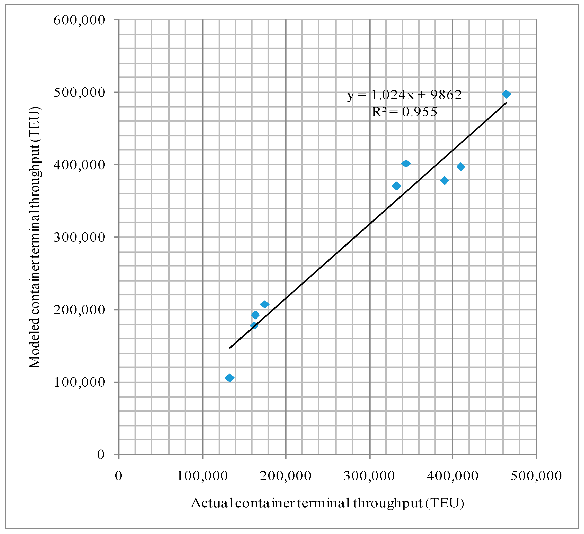
A validation test was needed to check the goodness of fit of the model with the data. The validation model, which simulated the current situation of the YREB case, where only inland waterway terminals were included and no environmental policy control instruments were considered, was developed. The inland railway terminals were not considered, since most inland railway terminals are under planning or under construction in the YREB region. Figure 3 shows the results of the validation model, in aspect of terminal choice. The performance of terminal choice was evaluated by comparing the modeled throughputs of inland waterway terminals, with the actual throughputs of these terminals for the YREB case. Figure 3 implies a high correlation coefficient (R² > 0.9) between calculated values and observed actual values, for inland terminals. From this perspective, the fit of the model was satisfactory.

3.2.ResultsAnalysis in Emissions Limitation Scenario

In emissions limitation scenario, the global emissions amount through the port-hinterland distribution network was limited with a range of ε. The parameter “ε” was lowered by 2.5% progressively, from the emissions result of the reference case, to the possible lowest emissions level that the YREB network could reach. The limitation percentage of 100% in

Table 2. Numerical results of flows indicators in emissions limitation scenario.

Limitation Percentage	Flows Through Direct Road and Intermodal Alternatives (103 TEU)				Flows Arrived at Gateway Seaports (103 TEU)
	Direct Road Flow	IWT-Only Transshipment	IRT-Only Transshipment	Inter-Terminal Transshipment	Shanghai Port				Ningbo-Zhoushan Port
					The Total	Road	Water	Rail	The Total	Road	Water	Rail
100.0%	5119	2071	776	477	4575	1990	2548	37	3867	3129	0	738
97.5%	5119	1857	998	469	4353	1990	2326	37	4089	3129	0	960
95.0%	5119	1947	1021	356	4329	1990	2302	37	4113	3129	0	984
92.5%	5119	1822	1149	353	4202	1990	2175	37	4240	3129	0	1111
90.0%	5119	1801	1202	321	4149	1990	2122	37	4293	3129	0	1164
87.5%	5119	1801	1238	285	4113	1990	2086	37	4329	3129	0	1200
85.0%	5119	1801	1274	249	4077	1990	2050	37	4365	3129	0	1236
82.5%	5119	1778	1337	209	3976	1990	1986	0	4466	3129	0	1337
80.0%	5119	1778	1392	154	3922	1990	1932	0	4520	3129	0	1391
77.5%	5119	1778	1449	97	3864	1990	1874	0	4578	3129	0	1449
75.0%	5119	1778	1507	39	3806	1990	1816	0	4636	3129	0	1507
72.5%	5119	1742	1582	0	3732	1990	1742	0	4710	3129	0	1581
70.0%	5119	1530	1794	0	3520	1990	1530	0	4922	3129	0	1793

, is the reference case. There were an additional 12 instances generated, except the reference case.

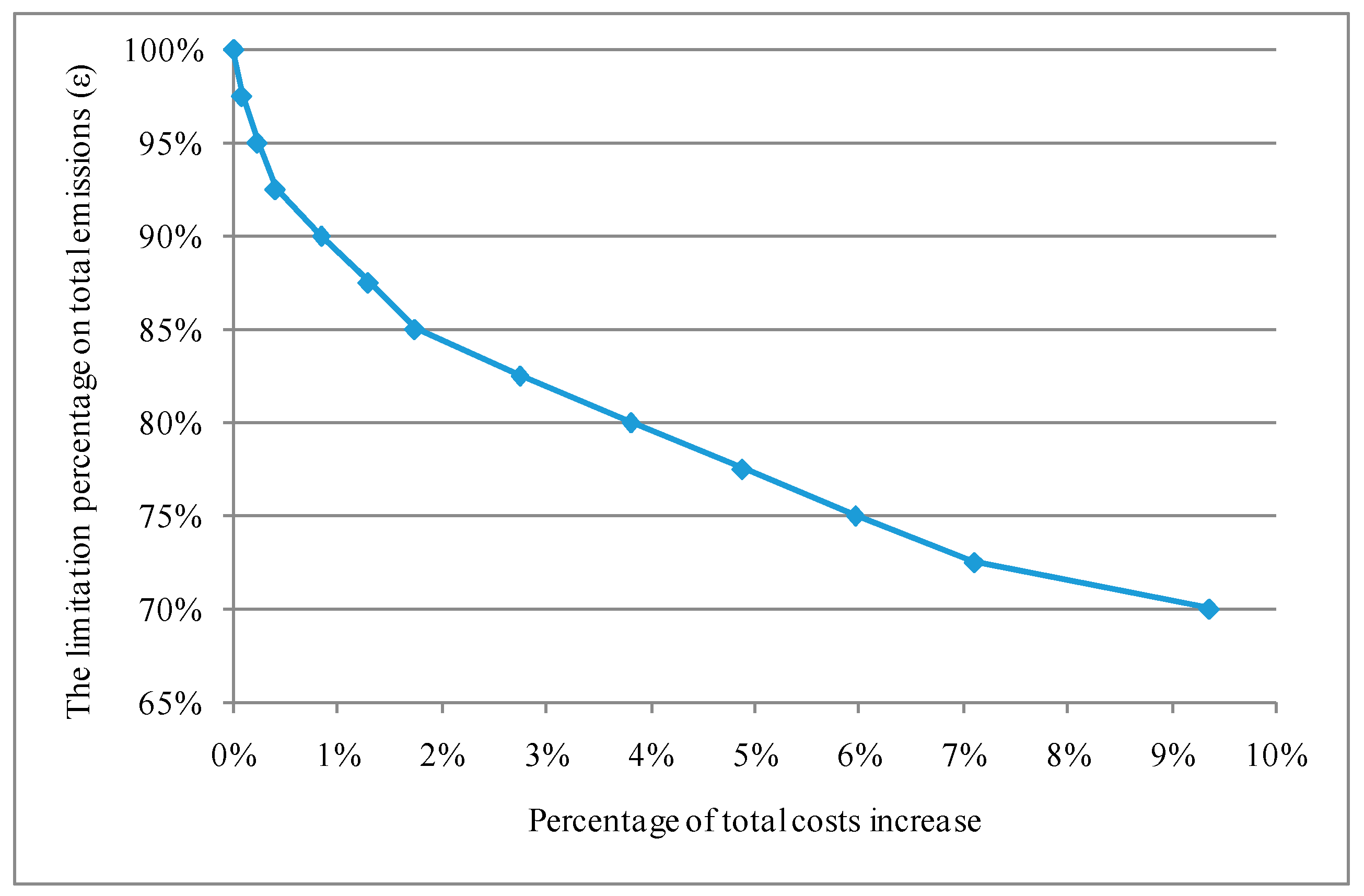
Figure 4 depicts the Pareto frontier obtained based on the results from all instances, which revealed the trade-offs between costs and emissions for the YREB case. Observing the slope of the Pareto frontier, a breaking point at the emissions limitation percentage of 85.0%could be identified, because the slope after this point started to drop remarkably. The reason could be investigated from the flows results in Table 2, which showed that more container flows preferred intermodal transport routes through the inland railway terminals to waterway terminals, with the tightening of limitation percentage. The IRT-only transshipment flows increased remarkably, especially below the limitation percentage of 85.0%, whilst flows on IWT-only and inter-terminal routes kept a declining trend.

It implies that 85.0% limitation is an inflection point, from which the increase of rail-only intermodal flows and the decrease of waterway-only intermodal flows as well as inter-terminal flows start to result in greater cost increase compared with that at high limitations. This is reasonable, since the rail transport features lower emissions rate while has higher transport cost rate than the waterway alternative. The changes in modal split at two gateway seaports in Table 2 also confirm that the increase of rail flows appears in the Ningbo-Zhoushan port. And it is also clear that the rail flows arrived at Ningbo-Zhoushan port grow significantly below the limitation percentage of 85.0%.

Overall, the emissions limitation instrument helped reduce carbon emissions by tightening the total emissions through the port-hinterland distribution network. The inflection point, from which higher total costs increase may occur for the same percentage of emissions reduction, would be offered to decision makers. It was investigated to be the limitation of 85.0%, in the YREB case. Moreover, if cost saving is targeted, the larger limitations (85% and over) would be required. Otherwise, the smaller limitations (under 85%) are suggested when environmental protection is more emphasized in the YREB case. Therefore, this scenario helped provide evident insights on the appropriate emissions limitation setting by a trade-off relationship analysis, specifically when the policy decision maker faces compromise solutions between cost saving and environmental protection.

3.3. Results Analysis inCarbon Tax PolicyScenario

The effects of introducing carbon tax policy on the proposed hinterland distribution network, were assessed in this scenario. The tax rate of $0, was the reference case without emissions consideration.

Table 3. Numerical results of cost, emissions, flow indicators in carbon tax policy scenario.

Tax Rate	Total Costs	Total Emissions	Flows Through Direct Road and Intermodal Alternatives (103 TEU)				Flows Arrived at Gateway Seaports (103 TEU)
($/Ton)	(Million US$)	(Tons)	Direct Road Flows	IWT-Only	IRT-Only	Inter-Terminal	Shanghai Port				Ningbo-Zhoushan Port
							The Total	Road	Water	Rail	The Total	Road	Water	Rail
0	2864	3,817,919	5119	2071	776	477	4575	1990	2548	37	3867	3129	0	738
5	2883	3,817,919	5119	2071	776	477	4575	1990	2548	37	3867	3129	0	738
10	2902	3,817,919	5119	2071	776	477	4575	1990	2548	37	3867	3129	0	738
15	2921	3,817,919	5119	2071	776	477	4575	1990	2548	37	3867	3129	0	738
20	2940	3,817,919	5119	2071	776	477	4575	1990	2548	37	3867	3129	0	738
25	2959	3,728,208	5119	1849	998	477	4353	1990	2326	37	4089	3129	0	960
30	2978	3,728,208	5119	1849	998	477	4353	1990	2326	37	4089	3129	0	960
35	2996	3,728,208	5119	1849	998	477	4353	1990	2326	37	4089	3129	0	960
40	3015	3,720,800	5119	1860	998	466	4353	1990	2326	37	4089	3129	0	960
45	3034	3,717,468	5119	1865	998	461	4353	1990	2326	37	4089	3129	0	960
50	3052	3,557,726	5119	1865	1106	353	4245	1990	2218	37	4198	3129	0	1069
55	3069	3,553,893	5119	1860	1111	353	4240	1990	2213	37	4203	3129	0	1074
60	3087	3,545,474	5119	1849	1122	353	4229	1990	2202	37	4214	3129	0	1085
65	3105	3,545,474	5119	1849	1122	353	4229	1990	2202	37	4214	3129	0	1085
70	3123	3,545,474	5119	1849	1122	353	4229	1990	2202	37	4214	3129	0	1085
75	3140	3,520,578	5119	1801	1170	353	4181	1990	2154	37	4262	3129	0	1133
80	3158	3,520,578	5119	1801	1170	353	4181	1990	2154	37	4262	3129	0	1133
85	3176	3,520,578	5119	1801	1170	353	4181	1990	2154	37	4262	3129	0	1133
90	3193	3,520,578	5119	1801	1170	353	4181	1990	2154	37	4262	3129	0	1133
95	3211	3,520,578	5119	1801	1170	353	4181	1990	2154	37	4262	3129	0	1133
100	3228	3,520,578	5119	1801	1170	353	4181	1990	2154	37	4262	3129	0	1133

gives the model outputs on costs, emissions, and flow indicators with the range of tax rates from $0 to $100 per ton of CO₂ emissions.

We found the total emissions drop, with the increase of the carbon tax rate from Table 3. This indicated that the tax policy in place, could help emissions reduction in the port-hinterland logistics network. The reason for this, were the changes in container flows routed through inland intermodal terminals. Interestingly, the direct road flows remained unchanged with the change in tax rate, which meant the direct road transport in this scenario did not have a competitive advantage not only in costs saving, but also in emissions reduction since it features the highest cost rate, as well as the highest emissions rate. Thus, the flow changes are focused on the rail intermodal and waterway intermodal alternatives. As seen in Table 3, the container flows routed through inland railway terminals show an uptrend (the 6th column), while the flows going through waterway terminals dropped (the 7th column). It indicated that more container freights were shifted to the lower emissions intermodal rail transport routes.

Regarding the flows at the gateway seaports, at tax rates of $0~$70, Shanghai Port absorbed more container freight than Ningbo-Zhoushan Port. However, higher tax rates from $75~$100, turn the tide of Ningbo-Zhoushan Port in the competition with Shanghai port by absorbing more hinterland container flows to the rail intermodal transport. Analyzing the modal split of containers in two gateway seaports, the only changes were the decreased flows that arrived in Shanghai Port by waterway (the 10th column) and the increased flows that arrived in Ningbo-Zhoushan Port by rail (the last column). It explained why the total rail intermodal flows in the seventh column grew, and why the total emissions of port-hinterland freight network reduced.

Figure 5 demonstrates the changes in total emissions and total costs, with the range of tax rates. The vertical axis represents the percentages of emissions reduction and costs increase, whilst the horizontal axis is the tax rate range. It can be seen clearly that there were three jumps in the performance of emissions reduction at tax rates of $25, $50, and $75 per ton, whilst the total costs kept a stable and linear increase trend. They are identified as the breaking points, after which very small environmental improvement can be achieved at the certain stages of tax rate range.

As a result, the introduction of carbon tax policy leads to emissions reduction. If the goal is for effective CO₂ emissions reduction, the appropriate carbon tax rates of $25, $50, and $75, which are the beginnings of the network emissions reduction to remain unchanged, it would be suggested to the decision maker in the YREB case. Additionally, it was found that only the flows of rail-road intermodal transport kept growing, while flows of direct road, barge-road, and inter-terminal options remained unchanged or decreased. The rail-road intermodal transport benefited more with the increase in tax rate. This scenario not only assessed the impacts of carbon tax policy on the decision making of shippers, but also helped to provide policy insights on setting an appropriate carbon tax rate.

3.4. Results Analysis inEmissionsTrading Scheme Scenario

This scenario discussed the effects of implementing emissions trading schemes on the YREB distribution network. The grandfathering theory was used to set a range of emission caps on the network. The grandfathering percentage of 100%, was the reference case. There were an additional 12 instances generated by capping the total emissions, with the range of grandfathering percentage at the interval of 2.5% from 100% to the possible emissions reduction goal (see

Table 4. Numerical results of emissions, cost, desired permit price and traded permits in emissions trading scheme scenario.

Grandfathering Percentage	Cap on Emissions (Tons)	Desired Permit Price($/Ton)	Total Emissions(Tons)	Total Costs (million $)	Number of Traded Permits(Tons)
100.0%	3,817,919	0	3,817,919	2864	0
97.5%	3,722,471	37	3,720,800	2866	−1671
95.0%	3,627,023	48	3,622,579	2870	−4444
92.5%	3,531,575	72	3,520,578	2875	−10,997
90.0%	3,436,127	136	3,277,093	2888	−159,034
87.5%	3,340,679	136	3,277,093	2901	−63,586
85.0%	3,245,231	137	3,243,944	2914	−1287
82.5%	3,149,783	318	3,115,594	2942	−34,189
80.0%	3,054,335	323	2,797,933	2973	−256,402
77.5%	2,958,887	323	2,797,933	3003	−160,954
75.0%	2,863,439	323	2,797,933	3034	−65,506
72.5%	2,767,991	389	2,757,919	3067	−10,072
70.0%	2,672,543	779	2,672,103	3132	−440

).

If the permit trading price is tested using some fixed values regularly under each given cap, the trend of emissions reduction should be similar to that from the tax scenario. Since in the minimizing of costs goal “O₁ + p·(O₂-cap)”, the component of “p·cap” is also fixed, due to which only the change in total costs results is incurred, compared to the cost objective “O₁ + p·O₂”. In this way, the optimization process in this scenario boils down to the process of the tax scenario. To get some different insights, and to find what trading price of emissions permits and which cap setting is useful for decision makers, we also tested the price with the fixed values repeatedly with a $1 increment, and attempted to find a watershed price. Taking the example of 97.5% grandfathering in Table 4, the result shows that when the model is tested with the permit trading prices from $1 to $36, the modeled total emissions generation is always higher than the given cap. It means that the value of “O₂-cap” keeps positive constantly, and logistics firms need to pay additional money to buy exceeding permits with the tested trading price p. However, the situation is reversed once the price of $37 can be traded, where the modeled emissions start to be lower than the cap. Such a trading price is the watershed price that is desired by logistics firms. It means that firms can get extra income by selling 1671 tons of the emissions permits, for example, in the instance of 97.5%. Such a desired trading price of emissions permits is searched for in all proposed grandfathering caps, and the modeled outputs under the required cap, as well as the desired price, are all showed in Table 4 and

Table 5. Numerical results of flow indicators in emissions trading scheme scenario.

Grandfathering Percentage	Flows Through Direct Road and Intermodal Alternatives (103 TEU)				Flows Arrived at Gateway Seaports (103 TEU)
	Direct Road Flow	IWT-Only Transshipment	IRT-Only Transshipment	Inter-Terminal Transshipment	Shanghai Port				Ningbo-Zhoushan Port
					The Total	Road	Water	Rail	The Total	Road	Water	Rail
100.0%	5119	2071	776	477	4575	1990	2548	37	3867	3129	0	738
97.5%	5119	1860	998	466	4353	1990	2326	37	4089	3129	0	960
95.0%	5119	1947	1024	356	4326	1990	2299	37	4116	3129	0	987
92.5%	5119	1801	1170	356	4180	1990	2153	37	4262	3129	0	1133
90.0%	5119	1801	1262	261	4089	1990	2062	37	4353	3129	0	1224
87.5%	5119	1801	1262	261	4089	1990	2062	37	4353	3129	0	1224
85.0%	5119	1801	1274	248	4076	1990	2049	37	4366	3129	0	1237
82.5%	5119	1778	1355	191	3958	1990	1968	0	4484	3129	0	1355
80.0%	5119	1778	1546	0	3768	1990	1778	0	4674	3129	0	1545
77.5%	5119	1778	1546	0	3768	1990	1778	0	4674	3129	0	1545
75.0%	5119	1778	1546	0	3768	1990	1778	0	4674	3129	0	1545
72.5%	5119	1730	1593	0	3721	1990	1731	0	4721	3129	0	1592
70.0%	5119	1528	1795	0	3519	1990	1529	0	4923	3129	0	1794

.

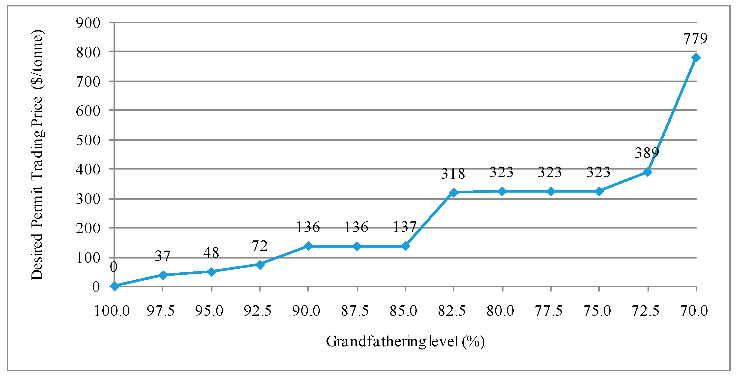
Analyzing the trend of desired permit trading price in Figure 6, the smaller grandfathering cap required, the greater permit price desired. The high prices, especially at the grandfathering levels below 85%, were too high to be accepted by corporations in practice, since they were difficult to realize in the real emissions trading market. Hence, the caps with a grandfathering percentage below 85% were not suggested for the YREB case.

The trends of changes in emissions reduction and costs increase, with the tightening of emissions caps, are depicted in Figure 7. They both maintained a climbing trend. Because the capping percentages below 85% did not perform well on the trading price desired, in the following analysis the percentages from 100% to 85% were focused on. There was a considerable growth in total emissions reduction of the YREB case, occurring at a range of 100% to 90%, by which a nearly stable phase was then followed until the percentage of 85%; whilst the total costs presented a slight increased trend. Thus, the cap with 90% grandfathering was identified as the breaking point, for the YREB case. The capping from 97.5% to 90% could be considered and suggested for the YREB case. These caps ensured relative apparent emissions reduction was obtained at lower desired permit trading prices, along with small costs increase.

Overall, this scenario particularly discussed the interaction of the grandfathering cap and trading price to discover the watershed price. The trend of watershed prices, under the range of grandfathering levels, revealed that the higher desired trading price was required with the lower cap set on the total emissions generated in the YREB network. To some extent, the goals of environmental protection and cost saving could be achieved simultaneously, when the emissions permit is traded with the watershed price for each cap level. This analysis implied that grandfathering percentages of 90% and over, were the best situations for the decision maker in the YREB case. The searched trading prices under these grandfathering levels seemed practical, and CO₂ emissions reduction can be achieved in return for a small social cost increase. Additionally, it was also found that the rail-road intermodal transport benefited more than the direct road, barge-road, and inter-terminal options. This implied that rail-road transport was the most competitive in the three-mode hybrid distribution network design, for the YREB case.

3.5 Sensitivity Analysis

To check the robustness of the model, sensitivity analysis was conducted on parameters of costs and emissions. These analyses in following sections, were performed to identify whether the results fluctuated strongly with test parameters. They also enabled us to explore the effects of these changes on the network behavior, for the YREB case.

3.5.1. Effects of Changing Cost Parameters

The effects of excluding time costs, changing cost parameters of modes of road, railway, and waterway on port-hinterland logistics network behavior are analyzed in this section.

Table 6. Effects of modifying cost parameters on network behavior.

Parameters	Total Costs	Total Emissions	Direct Road	IWT-Only Transshipment	IRT-Only Transshipment	Inter-Terminal Transshipment	Shanghai Port	Ningbo-Zhoushan Port
Excluding the time costs	−3.1%	0.0%	0.0%	0.0%	0.0%	0.0%	0.0%	0.0%
Road cost: +10%	6.4%	−2.3%	0.0%	−2.6%	2.6%	0.0%	−2.6%	2.6%
Road cost: −10%	−6.5%	−0.3%	0.0%	0.2%	0.0%	−0.2%	0.0%	0.0%
Railway cost: +10%	0.6%	0.4%	0.0%	0.3%	−0.3%	0.0%	0.3%	−0.3%
Railway cost: −10%	−0.8%	−3.0%	0.0%	−3.2%	3.2%	0.0%	−3.2%	3.2%
Waterway cost: +10%	1.7%	0.0%	0.0%	0.0%	0.0%	0.0%	0.0%	0.0%
Waterway cost: −10%	−1.7%	0.0%	0.0%	0.0%	0.0%	0.0%	0.0%	0.0%

gives the relative difference results of total costs and total emissions, and absolute difference results of percentage of flows distribution, compared with the reference case. For instance, excluding the time costs led to no change in flows distribution, which implied that emissions generation was not sensitive to the time cost parameter; whilst the total costs decrease was 3.1% compared to the reference case.

Road cost was the parameter that mostly influenced the network behavior on total logistics costs (+6.4% and −6.5% of relative variation) and total emissions (−2.3% and −0.3% of relative variation), when road cost increased 10% and decreased 10%, respectively. For example, in the “road cost increasing 10%” case, 2.6% of flows on IWT-only transshipment to the Shanghai gateway are shifted to IRT-only transshipment to Ningbo gateway, which is just the reason for the variations of total logistics costs and total emissions. Although flows on direct road routes are not influenced, the increase of road cost leads to a transfer of flows between intermodal options because the costs of the pre-haulage part related to road transport are affected.

When the cost parameter of the main haulage part related to the rail is modified, a large variation of flow distribution between IWT-only and IRT-only transshipment is observed in the “railway cost increasing 10%” case. However, both the total logistics costs and total emissions present small sensitivity to the railway cost parameter. Moreover, the network behavior has slight sensitivity to the parameter of waterway cost, since the modifications of waterway cost do not cause changes in flow distribution and network emissions generation, whilst only the total logistics costs in these cases have small variations.

3.5.2. Effects of Changing Emissions Parameters

The effects of changing emissions parameters regarding transport modes comprising road, railway, and waterway, on both total costs and emissions are discussed in this section. This study considered six emissions-related sensitivity tests, in which the CO₂ emissions parameters of three transport modes were increased by 10% and decreased by 10% (see Figure 8). Results showed that increasing emissions parameters of road, railway, and waterway transport shifted the Pareto frontier to the right, whilst reducing these parameters shifted it to the left. This revealed that the trade-off relationship between the objectives of total logistics costs and total CO₂ emissionswas nearly not affected, but both grow or drop because of the modified emissions parameters.

The largest gap was also observed for the tests on road transport, whether road emissions were increased or decreased. Total logistics costs and total emissions, are thus sensitive to the road emissions parameter. The second greatest came from the emission modification to the waterway transport, and the total costs and emissions had the least sensitivity to the rail emissions parameter. These results implied that the potential of emissions reduction and logistics costs decrease, for the YREB case, can be obtained from measures that help decrease road emissions and barge emissions; for example, investing in better roads, innovative technologies in increasing fuel efficiency of container trucks, and inland container barges and so on.

4. Discussion

Emissions limitation scenario analysis implied the trade-off relationship between total costs and total emissions. It was found that the tighter the limitation on total network emissions was, the greater the cost of satisfying the requested emissions limitation was caused. The finding was well in line with the results of Mostert et al. [33]. They applied a three-mode bi-objective intermodal network design model to the case of Belgium and reported that the cost effort for achieving the same amount of reduction of CO₂ emissions becomes larger. Although the optimal emissions limitation level was different from that of this paper, due to the differences in network design and the case data source, the findings are still comparable.

Tax policy analysis indicated that the increase in emissions tax rate, does cause network CO₂ emissions reduction. Meanwhile, the network costs increase with the growing of the tax rate. It was highly comparable with the findings of Zhang et al. [18]. If the only goal is to get effective CO₂ emissions reduction, the appropriate carbon price is needed, and $25, $50, and $75 for the YREB case in our paper were suggested. Zakeri et al. [40] reported tax prices of $5 and $55 were the breaking points, for a supply chain planning case in Australia. One of the results was very similar with that of this study. The different part of the results, may be partly due to the difference in case scope and data source. However, the finding is roughly comparable.

As for emissions trading scheme analysis in port-hinterland logistics planning problems, there are few similar or related researches in existing literature. There are some researches on supply chain modeling in a carbon trading environment, which tried to assess the impact of carbon price and carbon cap factors [46,47]. They mainly tested the impact of different carbon prices on supply chain behavior, and the results revealed that the trading price had a great influence on supply chain decisions. However, in our study, it was revealed that the higher desired trading price was required with the lower cap set on the total emissions generated. The interaction of the grandfathering cap and trading price was specifically investigated, to discover the watershed price. Similar results were not found in the literature, especially in the field of hinterland distribution network modeling. Moreover, the grandfathering percentages of 90% and over, were the best situations for the decision maker in the YREB case of this paper. These findings may be innovative, and they help enrich the existing literature.

5. Conclusions

This paper developed a generic model, for a three-mode hybrid port-hinterland freight intermodal distribution network with the environmental consideration. A bi-objective decision framework was built to provide environmental policy intervention analysis, including implementations of emissions limitation, emissions taxation policy, and emissions trading schemes. In each scenario, the relationships between economic efficiency and environmental goals were investigated. Although the mathematic model was built in the view of shippers, who are the ultimate users of the hinterland logistics network and bearers of policy implementation, the modeled results could provide some insights for the transportation sector and policy makers, in terms of flow distribution and emissions policy effects.

As for the flow distribution through the applied YREB case, it was found that the flows on direct road from inland cities to gateway ports were not influenced in all policy scenarios. Instead, great changes in flows between intermodal routes occurred and rail transport benefited more under all policy intervention scenarios. Regarding policy insights, the conflict between logistics costs and carbon emissions, differs from policy to policy. Some inflection points were identified under various policy implementations: (1) the limitation of 85.0% on network emissions is suggested as the optimal limitation level, when the emissions limitation instrument is introduced; (2) carbon tax rates of $25, $50, and $75 per ton are viewed as breaking tax levels, which lead to considerable emissions mitigation; and (3) grandfathering percentages of 90% and over, are suggested as appropriate emissions permit cap levels, at which the searched trading prices are practical. These findings offer decision support on port-hinterland distribution network behavior, when different environmental policies are implemented. In the end, the sensitivity analysis on cost and emissions parameters both revealed that the road is the transportation mode to which the behavior of port-hinterland distribution network and trade-off relationship between economic and environmental objectives, are mostly sensitive.

Although the model and its application serve the supportive role of emissions control policies in reducing carbon emissions through the port-hinterland distribution network, they also point out one limit on policy setting. This paper had not considered some instruments that are also aimed at reducing emissions, for example, subsidy of intermodal chains, which also influences the route choice of shippers in cost performance. In addition, maritime shipping network has impacts on the port-hinterland connections and the decisions of shippers, especially in the context of the Belt and Road Initiative originally proposed by China [48]. Thus, another extension of the research may be applying the methodology toglobal supply chains to explore the understanding of the policy impacts on a global scale.