Article

Stochastic Electric Vehicle Network Considering Environmental Costs

1
School of Transportation, Southeast University, Nanjing 211189, China
2
Department of Engineering, National University of Singapore, Singapore 117576, Singapore
3
Jiangsu Key Laboratory of Urban ITS, Southeast University, Nanjing 211189, China
4
Collaborative Innovation Center of Modern Urban Traffic, Southeast University, Nanjing 211189, China
*
Authors to whom correspondence should be addressed.
Sustainability 2018, 10(8), 2888; https://doi.org/10.3390/su10082888
Submission received: 20 June 2018 / Revised: 8 August 2018 / Accepted: 10 August 2018 / Published: 14 August 2018
(This article belongs to the Special Issue Travel Behaviour and Sustainable Transport of the Future)

Abstract

:
In recent years, many countries have published their timetables to promote electric vehicles. Many researches have focused on the benefits of electric vehicles. Compared with gas vehicles, electric vehicles are more suitable for modern cities, because they are considered to be environment-friendly by the public. Hence we pay attention to the environmental costs of electric vehicles. In this paper, an electric vehicle network is established. To analyze this electric vehicle network, we define environmental costs for the network and propose a stochastic user equilibrium model to describe drivers’ route choice behavior. An algorithm is proposed to solve this model. The model and the algorithm are illustrated through a numerical example. We test the calculation feasibility of the proposed model and the computational efficiency of the proposed algorithm via this numerical example. A comparative analysis is conducted to show the benefits of introducing electric vehicles into traffic networks. With the sensitivity analysis, we also reveal the relationship between people’s environmental awareness, the quantity of electric vehicles and the environmental costs of the overall traffic network.

1. Introduction

An electric vehicle (EV) network may be one of the topics which the public is focused on. This is because many countries have announced their incentivizing policies for electric vehicles. After England declared its intention to forbid the sale of gas vehicles (GVs) from the year 2040 onwards in July 2017, France, Germany and Netherlands also pronounced their intentions to cease selling gas vehicles. As of January 2018, more than six developed countries and 18 states in the United States have made their timetables for substituting gas vehicles with electric vehicles (EVs). With such a large number of EVs, not only an environment-friendly traffic network but also a brand-new travel mode will come into being. In the academic literature, researchers call it the electric vehicle network. The electric vehicle network can only come into being when there is a considerable quantity of electric vehicles in the traffic network. If electric vehicles only occupy a very small proportion of the network, they will have little impact on the whole network. For example, an electric vehicle network had not yet been developed when the first electric vehicle Citicar was produced by Vanguard-Sebring in 1973. 2% of the vehicle market which is ensured by the Zero Emissions Mandate in California in 1998, also has negligible effects on the network. However, the dream of an electric vehicle network is going to be realized, since many countries have released their announcements to substitute GVs with EVs in a few decades. These announcements published by governments guarantee the uptake of a large quantity of electric vehicles, which will actualize the electric vehicle network in the very near future. Thus, a reasonable number of electric vehicles are considered in this paper, varying from 20% to 80%.
A recent research article predicted that there would be 13~40 million EVs of a total of 300 million vehicles operating on the U.S. roads over the next decade [1]. Many researchers predicted that EVs which rely entirely on battery will provide an ultimate solution for personal transportation [2]. Such a large number of EVs mean not only a considerable market but also an environmentally-friendly modern world. The critical reason for many countries to develop timetables for electric vehicles is that electric power is more environmentally-friendly than gasoline and is easy to obtain. An EV is much more beneficial to the environment compared with a GV. However, in regard to the aggregate quantities of drivers, the results can differ. Actually, on the scale of traffic networks, we still do not know whether EVs are environmentally-friendly to the overall traffic network. This is because the traffic network is a non-linear complex system. When drivers take environmental costs into consideration, their travel behavior will be changed, which affects the environmental costs in turn. Moreover, in the scale of traffic networks, there is no explicit definitions of the environmental cost of private vehicles or urban traffic networks. Both of these problems lead to the ambiguity of the influences which EVs impose on the environment.
The environmental costs and drivers’ travel behavior should be considered simultaneously, which complicates our research goals. Because of the interrelation of environmental costs and drivers’ travel behavior, it is not possible to analyze each of them independently. Hence the equilibrium theory needs to be employed. What is more, travelers only consider their internal costs, i.e., the generalized travel costs hereafter, which affect their own benefits. However, the environmental costs are external costs. This means that the environmental costs do not directly harm travelers’ benefits. Thus, when analyzing travelers’ environmental costs, we need to take their environmental awareness into consideration, which further complicates our research goals. As we are aware, different levels of environmental awareness will lead to different generalized travel costs and subsequently different travel behavior and flow patterns. Remember, in urban traffic networks, there are in general millions of travelers. Both the quantities of travelers and the requirements of equilibrium in generalized travel costs increase the complexity of our problems.

1.1. Related Studies

As mentioned above, travelers only care about their generalized travel costs. To the travelers, the most appealing benefit of motorization is the generalized costs, which include travel time costs, monetary costs, operating costs and environmental costs. There has been lots of research focusing on the travel time costs, monetary costs and operating costs [3,4,5,6]. This research proposed generalized costs which contain travel time costs, monetary costs and operating costs of vehicles, respectively. For example, Jiang and Xie proposed a generalized cost for EVs which contained travel time costs and operating costs [6]. Sun et al. proposed a generalized cost which considered travel time costs, operating costs and monetary costs, for buses [5]. Besides these costs mentioned above, the environmental impacts of vehicles have recently been a topic of great interest [7,8,9,10,11]. The environmental impacts on special vehicles and carriers can be found as well [12,13]. However, the environmental costs of private vehicles or of urban traffic networks have not been focused on. To consider the environmental impacts of EV networks, the environmental costs are indispensable.
The research problem of interest in this article is a network equilibrium problem for an EV network. To describe and solve this problem, traffic network equilibrium problems and drivers’ route choice behavior should be considered. Some equilibrium models were employed to solve the network equilibrium problem in literature [5,14,15,16]. For example, one of the most famous forms of equilibrium is called the user equilibrium (UE) which was proposed to describe Multiplayer Non-cooperative Competition behavior among the drivers in urban traffic networks. Another useful tool is an improvement of UE: Stochastic user equilibrium (SUE), which describes the network more practically and precisely [17]. In this paper, we employ SUE to describe the drivers’ route choice behavior.

1.2. Objectives and Contributions

We focus on the environmental costs of electric vehicles. In this paper, we define the environmental costs for both gas vehicles and electric vehicles to fill the gaps in the literature and analyze the environmental costs through a comparative analysis and a sensitivity analysis.
We consider the environmental costs of EVs in an electric vehicle network. In this paper, we are curious about the influence, especially the environmental influence, made by EVs in traffic networks. Thus, we analyze the environmental impacts of EVs by proposing an SUE model for EV networks. The major contributions of our research are listed as follows:
We take environmental costs into consideration in the scale of traffic networks. An electric vehicle network is established. The environmental costs for the travelers in the EV network is related with travelers’ environmental awareness.
To solve our problem of describing the environmental costs in EV network, we propose a logit-based SUE model for EV network with environmental costs. An algorithm is proposed to solve this model.
A large-scale network is used as a numerical example to test the computational efficiency of this algorithm. Moreover, the comparative analysis and the sensitivity analysis are employed to illustrate the test results. Through our work, we verify the environmental impacts of EVs. The results can be used for governments to promote EVs in a private vehicle market.

2. Methodology

2.1. Modeling

In this section, we will propose a model to describe the electric vehicle network and its properties. The most relevant properties of an EV network in this paper are its environmental costs and its travelers’ route choice. A traffic network is commonly considered to be a non-linear complex system. This is because the flow pattern of the network is not determined by one specific traveler, but is instead determined by all travelers’ route choice behavior. This is the reason why the theory of urban traffic network, or the so-called traffic assignment problem (TAP), was proposed in 1980s. In this section, the environmental costs and the travelers’ route choice in electric vehicle network are discussed. By doing this, we conclude by covering the differences between an EV network and a GV network and propose our model for electric networks in this section.

2.1.1. Environmental Costs

Compared with gas vehicles, electric vehicles hardly create contaminants while traveling. However, generating electricity does produce contaminants. Thus, we define the unit contaminant of EV as the contaminant produced by generating the electricity which is consumed by EV when EV travels a unit of distance. In modern days, in most power plants, the contaminants are under centralized treatment. So, in general, the contaminants produced for generating electricity are much less harmful than those produced directly by consuming gas. Furthermore, in many countries, a large amount of electricity is produced by clean energy, such as nuclear energy and wind energy. For example, in France, more than 70% electricity is produced by nuclear [18]; the United States produces the most wind-generated electricity in the world [18]. Thus, although it is hard to describe the contaminant of EV throughout different countries with a fixed number, the unit contaminant of EV is definitely lower than that of GV. Here, in this paper, we use a parameter E e to denote the unit contaminant of EV and E g to describe that of GV, where E e < E g . To simplify the discussion, for gas vehicles we assume E g = 1 . Note that in different countries, E e may vary because of their electricity structure.
Now we can define the link performance function, which describes the generalized costs in overall traffic network, with the consideration of environmental costs. Here we employ the famous Bureau of Public Road (BPR) function and make a revision of it. The revision makes the BPR function suitable for describing environmental costs in the overall traffic network. We give out the expression of the revised BPR function as follows:
t a , i ( x a ) = d a ( 1 + 0.15 ( i x a , i C a ) 4 ) + d a E i  
where the first term on the right side refers to the travel cost while the second term refers to the environmental costs; for each link a, d a is a constant which denotes the physical length of link a.
Equation (1) describes the generalized cost on link a. This first term on the right side is the travel time cost. It denotes the time a vehicle may cost when the vehicle is traveling through this link. Note that the original BPR function is not suitable for the EV network. This is because it does not take EVs into consideration. Through our revision, both GVs and EVs are considered. The second term denotes the vehicle’s environmental cost when the vehicle is traveling. We note that the environmental cost of a vehicle is determined only by the distance it travels and the unit contaminant. This is because in traffic networks, although the gasoline/electricity consumed when idling may be different from that consumed when traveling, the idling of vehicles always happens at the end of a link. So, when considering the environmental cost as per link, we can regard idling as a part of traveling and calculate the environmental cost for each link by multiplying the link’s length by the unit contaminant of vehicles. Thus, since the length of each link can be easily measured, in urban traffic network, the environmental cost a vehicle endures can be directly determined by the length d a of the links that it travels through and the unit contaminant E i . Similar conclusions can also be found in other research on EVs [6,19].
With the help of Equation (1), it is enough to describe the generalized cost for EV network. However, for travelers, the generalized cost needs to be further modified. This is because travelers always make their decisions while only considering their own costs. Actually, the environmental cost is an external cost, and it does not directly affect travelers. That is to say, if a traveler produces contaminants when traveling, this does not directly harm his/her own benefits. Only when the traveler has environmental awareness, can the non-environmentally-friendly behavior provide him/her with a moral punishment which becomes an internal cost that he/she cares about. Unfortunately, travelers only consider their internal costs. Thus, we design a parameter A to describe the environmental awareness. The generalized cost becomes
t a , i ( x a ) = d a ( 1 + 0.15 ( i x a , i c a ) 4 ) + d a A E i  
where A denotes the average level of citizens’ environmental awareness in the network.
When considering travelers’ behavior, we describe their generalized costs with (2) rather than (1).
Between each OD pair, there are many paths for travelers to use. Each path is made up with several end-to-end links. Apparently, the cost of a path, which is called the path cost, is the summation of the costs of the links belong to this path. For example, if a path consists of two links, the path cost equals to the cost of the first link plus that of the second one. Hence we define the path cost of traveler i on the path k between OD pair rs more precisely for EV network as:
c k , i r s = a δ a . k r s t a , i ( x a )  
where δ a . k r s is the link-path incidence parameter, where δ a , k r s = 1 if link a belongs path k between OD pairs r s , and δ a , k r s = 0 , otherwise.

2.1.2. Logit-Based Stochastic User Equilibrium

In this paper, we analyze the impact of EVs on the overall network. Hence a theory of traffic network is needed. The theory of traffic network is a foundation of much traffic research, for example, on network design problems (NDPs) [20], traffic assignment problems (TAPs) [21], and route choice analysis [22,23]. In this paper, the TAP and the theory of traffic network are employed as tools to consider our problems with respect to the electric vehicle network.
In conventional networks (i.e., gas vehicle networks), researchers have proposed a number of models to describe the network. One of the most famous models known as logit-based stochastic user equilibrium (SUE) is employed and revised here for agreement with electric vehicle networks.
The logit-based SUE was first proposed by Daganzo and Sheffi to describe travelers’ route choice behavior in TAPs [21]. It describes the principle travelers hold when traveling: Travelers always choose their paths which they perceive as the paths with the lowest generalized costs. And, as we mentioned before, the generalized costs are always internal costs. However, different travelers have different perception levels about their internal (path) costs. To solve this problem, the logit-based SUE was proposed. The logit-based SUE model calculates the probability of path chosen by the drivers in terms of the path costs perceived by them. The lower a path cost is perceived to be by the drivers, the larger probability the path will be chosen to travel on. Details about the logit-based SUE model can be found in a great deal of research, such as Reference [18]. However, the original logit-based SUE model is not suitable for electric vehicle networks because there are two types of vehicles (or drivers). Thus, we propose a revision of the original logit model and make it fit for electric vehicle networks.
P k , i r s = exp ( θ i c k , i r s ) l exp ( θ i c l , i r s ) ,   l K r s  
where θ i denotes the drivers’ perception levels for path costs, i = e for electric vehicle drivers and i = g for gas vehicle drivers.
Equation (4) is a slight revision of the logit model, which divides the vehicles into two types: EVs and GVs. Then, we can calculate their path choice probabilities respectively. θ i is the perception level of the drivers. It is a critical parameter for SUE which was first proposed by Reference [21]. This parameter describes the perception levels of different types of drivers. Since drivers have their own preferences, different types of drivers may have different perception levels. Details about this parameter can be seen in Reference [21]. Since there is currently no obvious evidence to prove that GV drivers and EV drivers are different in perception ability, we assume the perception parameters of electric vehicle drivers and gas vehicle drivers are the same, i.e., θ e = θ g .
For vehicle i , the path flow can be obtained:
  f k , i r s = q i r s P k , i r s  
where q i r s denotes the traffic demand of vehicle i .
Note that in Equation (4), the denominator also has a realistic meaning. Since the logit-based model was originally proposed with respect to the theory of utility maximization [24,25], the denominator of Equation (4) actually denotes the summation of the utility of all the paths between the OD pair, i.e.,
u i r s = l exp ( θ i c l , i r s )  
According to the definition and the expression of Equation (6), we can easily determine that the utility of the paths is in negative correlation to their generalized costs. That is to say, a larger utility of a specific OD pair means the travelers between this OD pair suffer smaller generalized costs. This property of u i r s will be utilized later in Section 3.2 to analyze whether the existence of EVs is beneficial to the travelers.

2.1.3. Stochastic User Equilibrium for EVs with Environmental Costs

After introducing and employing the above revisions, we subsequently propose our model as follows:
min z ( x ( f ) ) = a i ( 0 x a , i t a , i ( ω ) d ω ) + i [ 1 θ i r s k f k , i r s ln f k , i r s ]  
Subject to:
k f k , i r s = q i r s  
x a , i = r s k f k , i r s δ a , k r s  
  f k , i r s 0  
The objective function (7) employs a framework of logit-based SUE model for traditional traffic network. The critical difference between Equation (7) and the objective function of traditional SUE model is the term of 0 x a , i t a , i ( ω ) d ω . In Equation (7), the costs of both GVs and EVs are taken into consideration, and both the travel time costs and the environmental costs are taken into consideration. Traditional SUE models did not achieve these two goals.
Equation (8) is the constraint of flow conservation. It ensures that the sum of the path flow f k , i r s equals to the traffic demand q i r s ; Equation (9) is the definition constraint of link flows in terms of path flows; Equation (10) is the nonnegative constraint which makes sure the path flows are nonnegative.
The equivalence of this model and the uniqueness of its solution can be easily proved by employing Lagrange function and the convexity of this model. The proofs for traditional SUE model can be seen in other research [18,21]. And since our revision does not change the convexity of the model, the equivalence and the uniqueness proofs remain unchanged and are omitted here.

2.2. Algorithm

The SUE model we proposed is a non-linear programming (NLP) model, which is usually hard to solve. Luckily, there are a few dedicated algorithms for solving SUE models efficiently. In this section, we employ the method of successive average (MSA) which is used to solve traditional SUE problems. MSA was first introduced into traffic networks in the 1960s [26]. It transforms this NLP into a shortest path problem which can be solved easily by the Dijsktra algorithm [26]. Here, we propose a revised MSA algorithm to solve our model.
We revise the MSA algorithm for the logit-based SUE for EV network with environmental costs:
Step 1: Initialization
Let x a , i ( 0 ) = 0 , calculate the free-flow link cost t a , i ( 0 ) and the path cost c k , i r s , ( 0 ) by (2) and (3), where i = e for electric vehicles and i = e for gas vehicles. Obtain the initial path flow f k , i r s ,   ( 0 ) by (4) and (5).
Step 2: Update
Update x a , i ( n ) = r s k f k , i r s ,   ( n ) and calculate t a , i ( n ) and c k , i r s , ( n ) by (2) and (3).
Step 3: Finding the search direction
According to c k , i r s , ( n ) obtained in Step 2, we calculate the auxiliary path flow g k , i r s ,   ( n ) by (4) and (5).
Step 4: Moving
  f k , i r s ,   ( n + 1 ) = f k , i r s , ( n ) + α n ( g k , i r s ,   ( n ) f k , i r s , ( n ) )  
where α n = 1 / n which denotes the step length of moving.
Step 5: Convergence criterion
If
i r s k ( f k , i r s ,   ( n + 1 ) f k , i r s ,   ( n ) ) 2 i r s k f k , i r s ,   ( n ) ε  
where ε is a pre-given accuracy, the algorithm stops and x a , i ( n ) is the solution (i.e., link flow at SUE). Otherwise, let n = n + 1 and return to step 2.
To test our model and algorithm more clearly, in the next section, we propose an example which is the Sioux-Falls network. We use all nodes, links and OD pairs of this large-scale network to test the computational efficiency of our model.

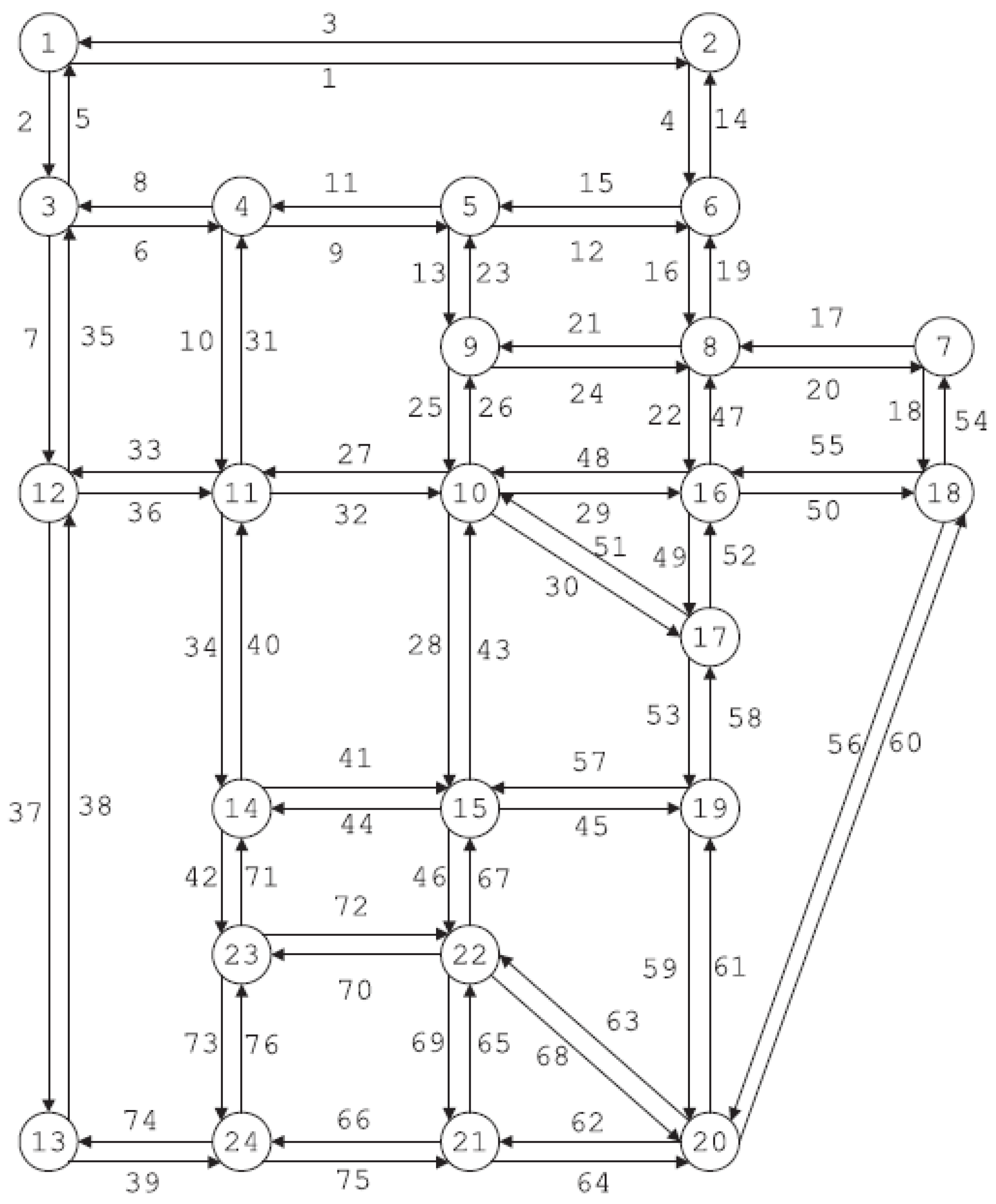
3. Numerical Example

In this section, we test our model and algorithm through a large-scale network which is frequently used as numerical examples in traffic network researches. Besides the disclosure of the test results and the comparison between the flow pattern of the traditional traffic network and that of the EV network, calculation feasibility and sensitivity analysis of our model are also conducted. Since traffic network problems are usually large-scale problems in computation, the calculation feasibility of our problem will be tested. Furthermore, our problem involves some parameters which play an important role in our model, and a sensitivity analysis will be conducted. All these works are based on the large-scale network and are conducted on an ordinary personal computer. Our experiments may be repeated with similar data and tools.

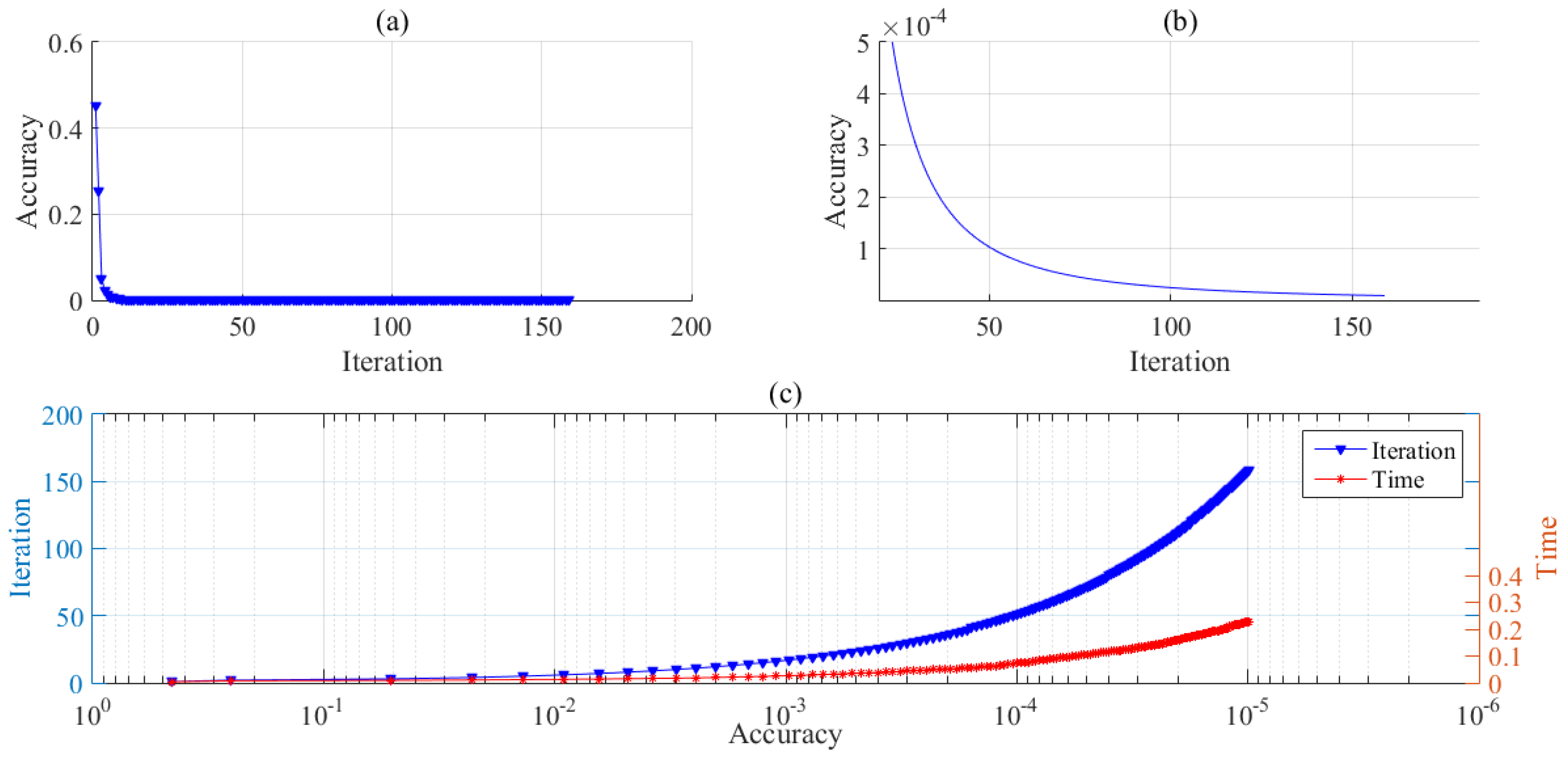
3.1. Calculation Feasibility

For the convenience of expression, we discuss the calculation feasibility first.
As we know, transportation problems and TAPs are usually large-scale problems in computation. For example, in the numerical example of Reference [27], the Sioux-Falls network is considered. In that example, the notation δ a , k r s actually denotes 1342 × 76 parameters.
Because of the large scales of TAPs, the most critical problem we concern is the calculation feasibility. In our model, not only traditional vehicles (i.e., gas vehicles) but also EVs need to be considered. Furthermore, because of the introducing of EVs, both the quantities of variables and parameters double compared to the usual quantities. The scale of the model becomes quite large. Hence we are concerned with the computational efficiency of our algorithm more than anything else.
To test our problem, we illustrate a typical large-scale network, the Sioux-Falls network, as our example. The Sioux-Falls network is a famous network which is frequently used in testing TAPs. It has 24 nodes, 76 links and 528 OD pairs as Figure 1. The length d a of each link is the same as the input data proposed by Reference [28]. The links’ capacities and traffic demand follow those proposed by Reference [29].
To show the efficiency of our algorithm, we test our example on an ordinary personal computer with a 2.60 GHz CPU, an 8 GB RAM and Windows 8.1 Enterprise 64-bit operating system. The model was coded with MATLAB.
In this example, we set the accuracy ε = 1 × 10⁻⁵, the perception levels of drivers θ e = θ g = 0.5 and the environmental awareness A = 2. The algorithm converges to the solution, see Figure 2.
In Figure 2, every marker represents an iteration of the proposed algorithm. For example, the 1st marker in Figure 2a illustrates the 1st iteration of the proposed algorithm achieves the accuracy of 4.5 × 10⁻¹. From Figure 2a and Table 1, we can see that the proposed algorithm converges quickly. At 6th iteration, the algorithm has reached the accuracy of 1%. After that, the curve of the convergence performance becomes gentle. However, although the convergence slows down, this algorithm is still quite efficient. Figure 2c shows the iterations and the computational time as per the accuracy this algorithm achieves. Note, for clearly illustration, we use a logarithmic abscissa in Figure 2c. It only takes 0.23 s and 159 iterations for the algorithm to converge at the accuracy of 9.9 × 10⁻⁶. What is more, Figure 2b is a closer view of Figure 2a. For better readability, in Figure 2b, we remove the markers and observe that the convergence curve of this algorithm is smooth. No “zig-zag” is observed during the whole convergence process. This means the accuracy of this algorithm is always getting higher along with iterations. These results show typical characteristics of MSA for SUE, which is as expected.
This large-scale example shows the computational efficiency of the proposed algorithm. Although both the quantities of variables and parameters double, the calculation is still efficient enough. One of the reasons may be that our revised algorithm takes advantages of MSA which is a dedicated algorithm to solve TAPs. With the help of MSA, we actually transform the NLP into a shortest path problem, which is extremely efficient for solving TAPs.

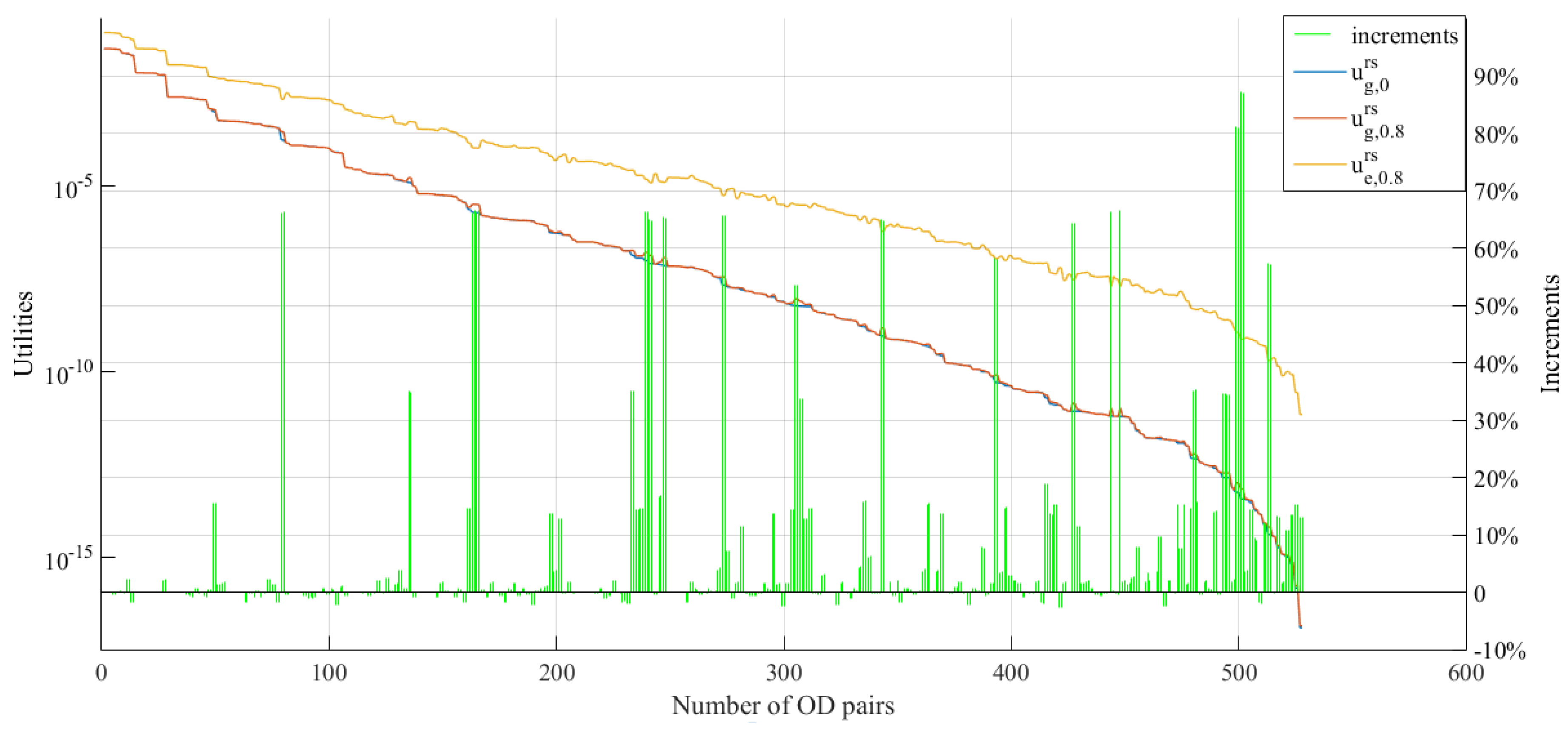
3.2. Comparative Analysis

The computational efficiency ensures our experimental results are obtained within a reasonable calculating time. Since we assume that a large number of EVs make a great impact on the overall traffic network, in this section, we will compare the flow pattern of the EV network with that of the traditional one.
We set the proportion of the EVs to all vehicles as 0.8, which means 80% vehicles are EVs, and keep other parameters the same as those in the former section. By doing this, we obtain the test results in the case that 80% vehicles are EVs (denoted as F 0.8 ). Then, we make the EVs vanish. It means all the vehicles in the network are gas vehicles to imitate the case of traditional traffic network (denoted as F 0 ). Since our model is a path-based model which uses path flow as its variables, we can actually compare the differences of each path in the network. However, as we mentioned above, in such a large-scale network there are usually thousands of paths. To list all the paths is unviable. Thus, as an alternative, we list the link flows instead. Considering that link flows are made up of path flows, thus, if we observe the changes in link flow, we know the path flows have changed. The test results are listed as follows in Table 2.
From Table 2, we find that the link flows of some links vary a lot, while others barely change. However, since traffic network is a non-linear system, it is not possible to claim which flow pattern is better. We can only tell that, due to the impact of EVs, drivers’ route choices do change. If we want to explore which flow pattern is more beneficial to travelers as per their generalized costs, we need to pick some OD pairs for deeper analysis.
In Sioux-Falls network, there are 528 OD pairs in total. It is impossible to analyze all of them as per their precise values at a time. Hence we choose 10 of them randomly and calculate their utilities as per (6). u i , 0.8 r s denotes the utilities of OD pair r s for vehicle i in the case of 80% vehicles are EVs, and u g , 0 r s denotes the utilities of OS pair r s for GVs when there are no EVs in the network. The results are shown in Table 3.
For the convenience for someone intending to repeat our experiment, we list the numbers of the picked OD pairs in Table 3. The numbers of OD pairs are in the same order as those in most research analyses which cited the Sioux-Falls network [30,31]. From Table 3, we find that the utilities of most OD pairs are improved. The exceptions are those of OD pairs 125 and 225, but the decrease in utility is not substantial. Note that the utilities of these OD pairs for GVs, a very slight decrease can be observed. Compared with the increment of utilities for EVs and the utilities of other OD pairs, the decrement is very small. We wonder whether this is a general phenomenon: To a certain degree, the introducing of EVs may help to increase the utilities, i.e., to reduce travelers’ generalized costs. To verify this statement, we list the utilities of all the OD pairs and their increments (or decrements), which can be seen in Figure 3.
To clearly illustrate the utilities of 528 OD pairs, we rank the OD pairs as per u g ,   0.8 r s in descending order. Thus, note the numbers of OD pairs in Figure 3 are not same as those in Table 3. We list the utilities u g ,   0.8 r s , u e ,   0.8 r s , and u g ,   0 r s of all 528 OD pairs in Figure 3 to analyze the changes in utilities after introducing EVs into the network. As shown in the legend of Figure 3, the blue, red and yellow lines denote u g ,   0 r s u g ,   0.8 r s and u e ,   0.8 r s respectively. We regard the line u g ,   0 r s as the baseline, the gaps between the line u g ,   0 r s and the line u g ,   0.8 r s represent the increments of utilities for GVs after introducing EVs into the network. Similarly, the gaps between u g ,   0 r s and u e ,   0.8 r s mean the increments of utilities for the EVs which were GVs before they changed their roles. Note, the utilities of 528 OD pairs range from 1 × 10⁻¹ to 1 × 10⁻¹⁷. To make our results more readable, we illustrate them in the logarithmic coordinate. The green bars in Figure 3 represent the ratio of the gaps between u g ,   0.8 r s and u g ,   0 r s to u g ,   0 r s , and they are in the linear coordinate.
It is as expected that the utilities for EVs are higher than those for GVs. This is because the generalized costs of EVs, which contain the environmental costs in them, are less than those of GVs. What is more, after introducing EVs, we observe that the utilities for GVs are also improved. The utilities for most of OD pairs are not lower than before, and some of them are obviously improved. However, one may argue that there are only slight gaps between the two curves which represent u g ,   0.8 r s and u g ,   0 r s in the figure. This is because they are in the logarithmic coordinate. To show the increments more clearly, we illustrate them with green bars in the linear coordinate in Figure 3. Since the utilities for each OD pair is not in the same order of magnitude, we make each bar to represent the ratio of the gaps u g ,   0.8 r s u g ,   0 r s to the baseline utilities u g ,   0 r s .
We observe that the utilities for GVs of most OD pairs are improved, and that some of the increments contribute nearly 90% of the baseline utilities. Although the utilities of some OD pairs decrease, the decrements are quite lower compared with the increments. The largest decrement only equals to 2.69% of the baseline utility. Moreover, the average of the increments is 11.8% of the baseline utilities, while that of the decrements is only 0.6%.
In this section, through a comparative analysis, we verify the benefits of the EV network. The existence of EVs in the traffic network improves the utilities, i.e., reduces the generalized costs, for not only the EV drivers (they were GV drivers before) but also stubborn GV drivers. It is indeed wise for the governments over the world to promote their encouraging policies for EVs.
Besides the above analysis, we are also curious about the extent of the impact of EVs and how much in total generalized costs will be reduced as per the quantity of EVs introduced into the traffic network. To answer this question, a sensitivity analysis will be conducted in the next section. The sensitivity analysis illustrates the impacts of the parameters which represent the proportion of EVs, citizens’ environmental awareness and the unit contaminant of vehicles in the proposed model.

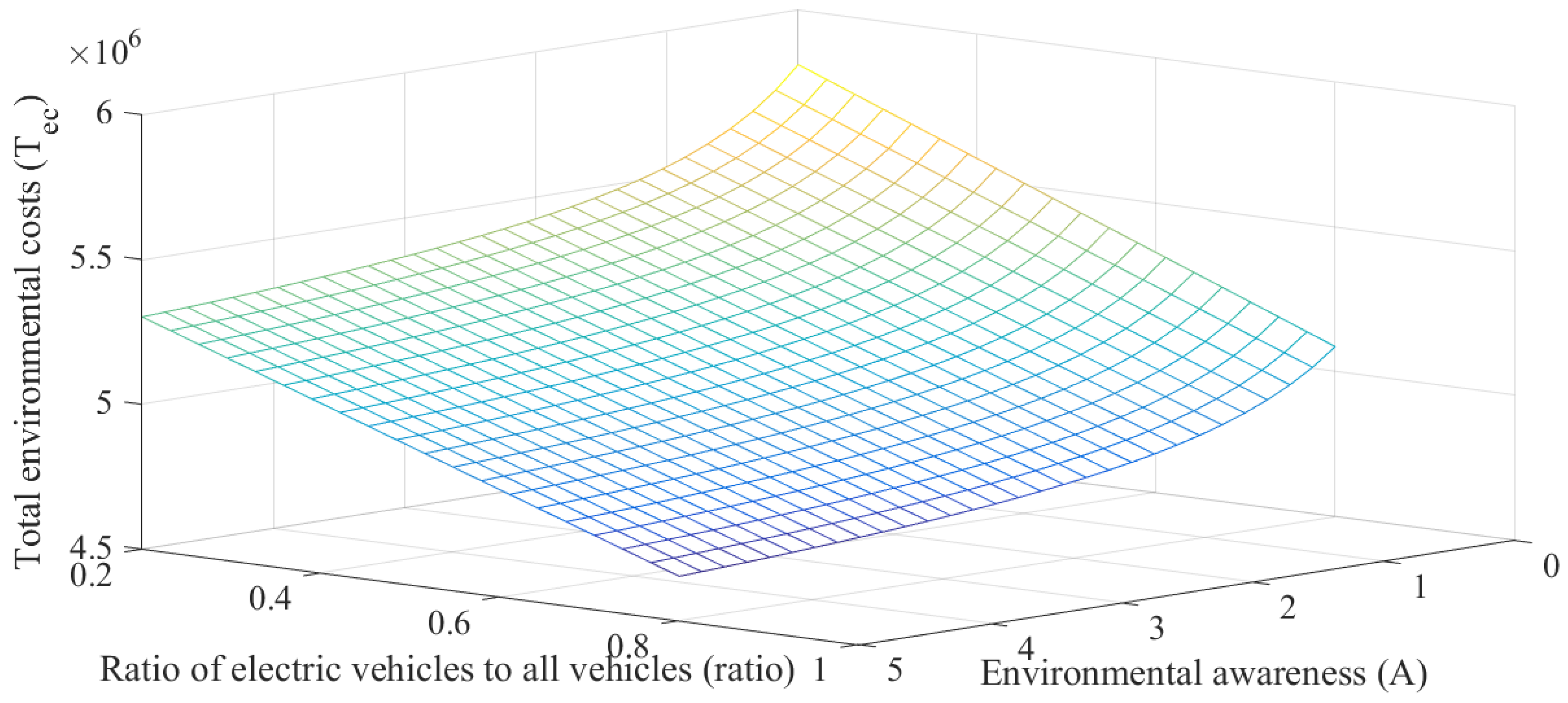
3.3. Sensitivity Analysis

Besides the test results and the computational efficiency, we also consider the parameters in the proposed model, especially the parameters related with environmental costs of the EV network. In this section, a sensitivity analysis is employed to discuss our test results. We are interested in how the environmental costs of the traffic network will vary, if we improve the proportion of EVs and citizens’ environmental awareness, or if reduce the contaminants when generating electricity.
The environmental cost of the overall traffic network is a summation of the environmental costs of all vehicles on all links in the network:
T e c = a i x a , i d a E i  
Note, here the environmental cost of a specific link a is not defined as d a A E i , since the environmental costs of the network is an objective fact. It is not an internal costs that reflected by people’s environmental awareness, thus, it has nothing to do with the parameter A to measure this objective fact. Therefore, we employ the second term d a E i of (1) rather than that of (2) to describe the environmental cost of the link.
The proportion of EVs in urban traffic network is usually considered related to citizens’ environmental awareness. Therefore, we analyze the environmental awareness A and the proportion of EVs together. The results are plotted in Figure 4.
As mentioned before, we fix the contaminant of EV E e = 0.8 and vary the proportion of electric vehicles from 20% to 80%. The environmental awareness A vaies in the range of 0~5. When A = 5, the internal environmental costs for the travelers equals to around 5 times of the travel time costs, which is considered large enough. From Figure 4, we can find that when r a t e and A get lower, T e c increases as a convex curve. This means when the proportion of electric vehicles and/or the environmental awareness decrease, the growth of the total environmental costs will increase at an accelerating rate. Thus, it is ideal for governments to improve people’s environmental awareness and the quantity of electric vehicles.
Figure 5 shows the relationship of the total environmental costs and the contaminant level of electric vehicles E e . Here, we take 30 values of E e varying in the range of [0, 1]. Each marker in Figure 5 represents a value of E e . Since the energy of EVs is electricity, E e reflects the contaminant produced in generating electricity. Hence E e getting lower means more clean energy is used to generate electricity.
According to Figure 5, when E e increases, the total environmental costs of the overall network increase. The results suggest that, if the unit contaminant of EVs can be reduced, the environmental costs made by EVs will decrease. That is to say, besides the people’s environmental awareness and the proportion of EVs, the unit contaminant of EVs also makes a great impact on the environment of traffic networks.

4. Discussions and Conclusions

Since the environmental effects of EVs have become topics of interest recently, our goal is to discuss the environmental costs of EVs qualitatively and quantitatively. We wanted to verify whether the existence of EVs would affect drivers’ route choice behavior and to what extent would EVs affect the environmental costs of the traffic network.
Although the environment-friendly attribute of EVs is one of the most significant reasons for governments to promote EVs, the environmental costs of EV networks were given little attention in previous studies. One of the strengths in this paper is that we propose a definition of environmental costs for both urban traffic networks and for the travelers. We consider private vehicles’ environmental costs in the scale of traffic networks, which was not previously achieved in literature. Furthermore, on the basis of the definition, we establish and analyze the EV networks with environmental costs. To imitate a real EV network and describe travelers’ route choice behavior, we propose a revised SUE model for the EV network and a revised MSA algorithm to solve our problems. By doing this, we actually help with evaluation of the policies promoting EVs. Due to the contribution of this model, governments can develop better policies to reduce both travelers’ travel costs and urban environmental costs. The calculation feasibility shows that the proposed model and algorithm are efficient enough to be applied in large-scale networks. A comparative analysis and a sensitivity analysis are conducted to test our results.
The findings of this paper are interesting. Through the comparative analysis, we observe an obvious difference between the flow pattern of the network with EVs and that of the network without EVs. The results suggest that the existence of EVs does affect drivers’ route choice behavior. Moreover, the existence of EVs reduces not only the generalized costs of EV drivers but also those of GV drivers. This finding is interesting because it is different from our intuition and is really beneficial to promoting EVs. We compare our findings with those in other researches [3,4,5,6] which focused on travel time costs, monetary costs or operating costs. Most of them did not conduct a similar comparison and did not achieve our findings. Through a sensitivity analysis, we further analyze the extent where EVs would affect the total environmental costs of the overall traffic network. The results suggest that a large number of EVs, a good environmental awareness of people and a low contaminant level of EVs can help reduce the environmental costs of the traffic network.
Our research is useful for practical policy purposes. First of all, since the existence of EVs reduces the generalized travel costs for both EV drivers and GV drivers, our research strengthens people’s confidence in believing that EVs can benefit their travels. Besides, our research suggests that governments pay attention to improving people’s environmental awareness and reducing the contaminant of EVs while they are promoting EVs. By doing these things simultaneously, governments will harvest a notable effect on reducing the total environmental costs of the urban traffic networks. What is more, according to our research, electric vehicle manufacturers can design better products, which are more environmental-friendly and with lower environmental costs, to cater to the customers with environmental awareness and the governments.
Moreover, because we employ the theory of traffic network in this model, some assumptions that will make the model more realistic and practical can be considered in the future. For example, since the travel distance of EVs is limited by the underdeveloped battery technology and travel patterns can change based on changing demands, the assumptions of distance limitation and elastic demand may be integrated into our EV network models in future research. In future research, we will take distance limitation and elastic demand into consideration. Both can help improve the proposed SUE model for EV networks with environmental costs. With their help, the models and results will be more practical and realistic.

Author Contributions

J.M. and L.C. collected the data; J.M. formulated the model and designed the algorithm; J.M. analyzed the data; L.C. approved the submission and publication; L.C. supervise the project; J.M. wrote the paper; D.L., Q.T. polished this paper.

Funding

This research was funded by National key research and development program (No. 2016YFE0206800), the National Natural Science Foundation of China (No. 51608115, No. 51378119 and No. 51578150), the Natural Science Foundation of Jiangsu Province (No. BK20150613), the Projects of International Cooperation and Exchange of the National Natural Science Foundation of China (No. 51561135003), the Scientific Research Foundation of the Graduate School of Southeast University (No. YBJJ184) and the Fundamental Research Funds for the Central Universities.

Acknowledgments

Comments provided by anonymous referees are much appreciated.

Conflicts of Interest

The authors declare no conflict of interest.

Notations

The following notations are used in the paper:
Sets
A r c set of links, where A r c = { a }
I set of vehicles, I = { i } , i = e denotes electric vehicles, i = g denotes gas vehicles
K r s set of route between origin-destination (OD) pairs r s , K r s = { k }
N o d e set of nodes, where N o d e = { n }
R S set of OD pairs, R S = { r s } , r , s N o d e
Parameters
A environmental awareness
c k , i r s travel cost of vehicle i on path k between OD pairs r s
C a capacity of link   a
d a physical length of link a
E contaminant of EVs
P k , i r s probability for vehicle i to choose route k between OD pairs r s
q i r s traffic demand of vehicle i between OD pairs r s
r a t i o ratio of the number of EVs to that of all vehicles in the network
t a , i generalized costs of vehicle i on link a
u i r s utility of OD pair r s for the vehicle i
θ i travel cost perception of vehicle i
δ a , k r s link-path incidence parameter, where δ a , k r s = 1 if link a is contained by path k between OD pairs r s , and δ a , k r s = 0 , otherwise
Variables
f k , i r s path flow of vehicle i on path k between OD pairs r s ; f = { f k , i r s }
x a , i link flow of vehicle i on link a ; x a = { x a , e ,   x a , g } , x = { x a }

References

  1. Addison, J. National Academies Predicts 13 to 40 Million Plug-ins by 2030. Available online: http://www.cleanfleetreport.com/plug-in-hybrids/national-academies-40-million-plug-ins (accessed on 19 May 2018).
  2. Lin, Z.; Greene, D.L. Promoting the market for plug-in hybrid and battery electric vehicles: Role of recharge availability. Transp. Res. Rec. J. Transp. Res. Board 2011, 2252, 49–56. [Google Scholar] [CrossRef]
  3. Jafari, E.; Boyles, S.D. Multicriteria stochastic shortest path problem for electric vehicles. Netw. Spat. Econ. 2017, 17, 1043–1070. [Google Scholar] [CrossRef]
  4. Yi, Z.; Smart, J.; Shirk, M. Energy impact evaluation for eco-routing and charging of autonomous electric vehicle fleet: Ambient temperature consideration. Transp. Res. Part C Emerg. Technol. 2018, 89, 344–363. [Google Scholar] [CrossRef]
  5. Sun, X.; Lu, H.; Chu, W. A low-carbon-based bilevel optimization model for public transit network. Math. Probl. Eng. 2013, 2013. [Google Scholar] [CrossRef]
  6. Jiang, N.; Xie, C. Computing and analyzing mixed equilibrium network flows with gasoline and electric vehicles. Comput. Aided Civ. Infrastruct. Eng. 2014, 29, 626–641. [Google Scholar] [CrossRef]
  7. Blackman, A.; Alpízar, F.; Carlsson, F.; Rivera, M. A contingent valuation approach to estimating regulatory costs: Mexico’s day without driving program. J. Assoc. Environ. Resour. Econ. 2018, 5, 15–21. [Google Scholar] [CrossRef]
  8. Zhu, W.; Yang, D.; Huang, J. A hybrid optimization strategy for the maintenance of the wheels of metro vehicles: Vehicle turning, wheel re-profiling, and multi-template use. Proc. Inst. Mech. Eng. Part F J. Rail Rapid Transit. 2018, 232, 832–841. [Google Scholar] [CrossRef]
  9. Bauer, G.S.; Greenblatt, J.B.; Gerke, B.F. Cost, energy, and environmental impact of automated electric taxi fleets in Manhattan. Environ. Sci. Technol. 2018, 52, 4920–4928. [Google Scholar] [CrossRef] [PubMed]
  10. Ioakimidis, C.S.; Thomas, D.; Rycerski, P.; Genikomsakis, K.N. Peak shaving and valley filling of power consumption profile in non-residential buildings using an electric vehicle parking lot. Energy 2018, 148, 148–158. [Google Scholar] [CrossRef]
  11. Tang, Y.; Zhang, Q.; Li, Y.; Wang, G.; Li, Y. Recycling mechanisms and policy suggestions for spent electric vehicles’ power battery—A case of Beijing. J. Clean. Prod. 2018, 186, 388–406. [Google Scholar] [CrossRef]
  12. Mazur, C.; Offer, G.J.; Contestabile, M.; Brandon, N.B. Comparing the effects of vehicle automation, policy-making and changed user preferences on the uptake of electric cars and emissions from transport. Sustainability 2018, 10, 676. [Google Scholar] [CrossRef]
  13. Park, E.; Lim, J.; Cho, Y. Understanding the emergence and social acceptance of electric vehicles as next-generation models for the automobile industry. Sustainability 2018, 10, 662. [Google Scholar] [CrossRef]
  14. Ma, J.; Li, D.; Cheng, L.; Lou, X.; Sun, C.; Tang, W. Link restriction: Methods of testing and avoiding braess paradox in networks considering traffic demands. J. Transp. Eng. Part A Syst. 2018, 144. [Google Scholar] [CrossRef]
  15. Kitthamkesorn, S.; Chen, A.; Xu, X.; Ryu, S. Modeling mode and route similarities in network equilibrium problem with go-green modes. Netw. Spat. Econ. 2016, 16, 33–60. [Google Scholar] [CrossRef]
  16. Mahmassani, H.S.; Chang, G.-L. On boundedly rational user equilibrium in transportation systems. Transp. Sci. 1987, 21, 89–99. [Google Scholar] [CrossRef]
  17. Guo, X.; Yang, H.; Liu, T.L. Bounding the inefficiency of logit-based stochastic user equilibrium. Eur. J. Oper. Res. 2010, 201, 463–469. [Google Scholar] [CrossRef] [Green Version]
  18. Barros, C.P.; Managi, S. French nuclear electricity plants: Productivity and air pollution. Energy Sources Part B Econ. Plan. Policy 2016, 11, 718–724. [Google Scholar] [CrossRef]
  19. Kuang, A.W.; Huang, Z.X. Stochastic user equilibrium traffic assignment with multiple user classes and elastic demand. In Proceedings of the 2010 International Conference on Intelligent Computation Technology and Automation, Changsha, China, 11–12 May 2010; pp. 394–397. [Google Scholar] [CrossRef]
  20. Ma, J.; Cheng, L.; Li, D. Road maintenance optimization model based on dynamic programming in urban traffic network. J. Adv. Transp. 2018, 2018, 11. [Google Scholar] [CrossRef]
  21. Daganzo, C.; Sheffi, Y. On stochastic models of traffic assignment. Transp. Sci. 1977, 11, 253–274. [Google Scholar] [CrossRef]
  22. Li, D.; Miwa, T.; Morikawa, T.; Liu, P. Incorporating observed and unobserved heterogeneity in route choice analysis with sampled choice sets. Transp. Res. Part C Emerg. Technol. 2016, 67, 31–46. [Google Scholar] [CrossRef]
  23. Li, D.; Miwa, T.; Morikawa, T. Modeling time-of-day car use behavior: A bayesian network approach. Transp. Res. Part D Transp. Environ. 2016, 47, 54–66. [Google Scholar] [CrossRef]
  24. McFadden, D. Conditional logit analysis of qualitative choice behavior. In Frontiers in Econometrics; Acedemic Press: New York, NY, USA, 1973; pp. 105–142. [Google Scholar]
  25. Luce, R.D. Individual Choice Behavior: A Theoretical Analysis; John Wiley & Sons: New York, NY, USA, 1959. [Google Scholar]
  26. Almond, J. Traffic assignment with flow-dependent journey times. In Vehicular Traffic Science; Elsevier: New York, NY, USA, 1967; pp. 222–234. [Google Scholar]
  27. Robinson, S. Springer Series in Operations Research; Springer: New York, NY, USA, 1997; ISBN 9781461271291. [Google Scholar]
  28. Leblanc, L.J. An algorithm for the discrete network design problem. Transp. Sci. 1975, 9, 183–199. [Google Scholar] [CrossRef]
  29. Wang, D.Z.W.; Lo, H.K. Global optimum of the linearized network design problem with equilibrium flows. Transp. Res. Part B 2010, 44, 482–492. [Google Scholar] [CrossRef]
  30. Wang, S.; Gardner, L.; Waller, S.T. Global optimization method for robust pricing of transportation networks under uncertain demand. In Proceedings of the 92nd Annual Meeting of Transportation Research Board to be Considered for Presentation and Publication in Transportation Research Record, Washington, DC, USA, 13–17 January 2013; pp. 33–48. [Google Scholar]
  31. Di, Z.; Yang, L.; Qi, J.; Gao, Z. Transportation network design for maximizing flow-based accessibility. Transp. Res. Part B Methodol. 2018, 110, 209–238. [Google Scholar] [CrossRef]
Figure 1. Sioux-Falls network.
Sustainability 10 02888 g001
Figure 2. Convergence performance of the revised MSA algorithm. (a) The accuracy of each iteration; (b) A closer view of (a); (c) The iteration and computational time as per accuracy.
Sustainability 10 02888 g002
Figure 3. Utilities of 528 OD pairs of Sioux-Falls network.
Sustainability 10 02888 g003
Figure 4. Sensitivity analysis of the parameters ratio and A .
Sustainability 10 02888 g004
Figure 5. Sensitivity analysis of the parameter E e .
Sustainability 10 02888 g005
Table 1. Accuracy at certain iterations.
IterationAccuracyIterationAccuracyIterationAccuracyIterationAccuracy
14.5 × 10−1103.0 × 10−3607.2 × 10−51201.8 × 10−5
35.1 × 10−2206.9 × 10−4804.0 × 10−51401.3 × 10−5
69.1 × 10−3303.0 × 10−41002.5 × 10−51599.9 × 10−6
Table 2. Comparison between link flows of EV network and those of traditional traffic network.
# of LinkF0.8F0# of LinkF0.8F0# of LinkF0.8F0
11790177427833982375362576185
22729270128729069605449195058
31792177529794983815556505911
42810280930213017965654675566
52728270031320731105759266157
63461346132827781755862566185
72921284033496349915930923011
83468346834619364626054565557
95178517335291328326130923011
103168307436494549696226492611
115156514837461946286335813397
123912397238459145986426392602
133759375039434443386539053932
142811280940618864596641744347
153931397741389438816782698277
165703570642331732076835823397
173214311643733370036938783902
184929506544388538747043504301
195722571245592561567133213210
203224312346823682427243574307
2178263347491549677329952848
224929498048794883807443174308
233719371849622863447541904368
2478163250565159127630062857
25732973025121291795
26728972705262296345
Table 3. Comparison of utilities of an EV network and those of a traditional traffic network.
# of OD Pair(rs)   u g ,   0.8 r s     u e , 0.8 r s     u g , 0 r s  
25(1–14)1.338 × 10−121.084 × 10−81.159 × 10−12
50(4–2)5.909 × 10−81.511 × 10−55.868 × 10⁻⁸
75(2–17)2.910 × 10−103.192 × 10−72.803 × 10−10
100(12–3)2.479 × 10−31.831 × 10−22.479 × 10⁻³
125(4–10)3.510 × 10−75.719 × 10−53.521 × 10⁻⁷
150(22–4)1.659 × 10−121.612 × 10−81.513 × 10−12
175(5–16)3.447 × 10−88.709 × 10−63.307 × 10⁻⁸
200(12–6)6.746 × 10−107.515 × 10−76.697 × 10−10
225(7–8)1.104 × 10−24.947 × 10−21.105 × 10⁻²
250(20–7)1.233 × 10−42.476 × 10−31.233 × 10⁻⁴

